Working Paper No. 281
Inference for Structural Impulse Responses
in SVAR-GARCH Models
Stefan Bruder
April 2018
University of Zurich
Department of Economics
Working Paper Series
ISSN 1664-7041 (print)
ISSN 1664-705X (online)
Inference for Structural Impulse Responses in SVAR-GARCH
Models
Stefan Bruder Department of Economics University of Zurich [email protected] April 3, 2018 AbstractConditional heteroskedasticity can be exploited to identify the structural vector autoregressions (SVAR) but the implications for inference on structural impulse responses have not been investigated in detail yet. We consider the conditionally heteroskedastic SVAR-GARCH model and propose a bootstrap-based inference procedure on structural impulse responses. We compare the finite-sample properties of our bootstrap method with those of two competing bootstrap methods via extensive Monte Carlo simulations. We also present a three-step estimation procedure of the parameters of the SVAR-GARCH model that promises numerical stability even in scenarios with small sample sizes and/or large dimensions.
KEY WORDS: Bootstrap; conditional heteroskedasticity; multivariate GARCH; structural impulse responses; structural vector autoregression. JEL CLASSIFICATION NOS: C12, C13, C32
1
Introduction
Identifying the structural vector autoregressive (SVAR) model is typically one of the crucial issues in structural impulse response analysis. The existing literature offers a plethora of different identification strategies; seeKilian and L¨utkepohl (2017) for an excellent overview. A recent strand of this literature exploits the presence of conditional heteroskedasticity for the identification of the SVAR model; see e.g.,Normandin and Phaneuf(2004),Lanne et al.(2010),
Bouakez and Normandin(2010) and Herwartz and L¨utkepohl(2014).
The presence of conditional heteroskedasticity entails that the standard assumption of an independent and identically distributed (i.i.d.) error process is no longer valid and needs to be replaced by weaker assumptions on the error process, such as weak stationarity and serial uncorrelatedness; see e.g.,L¨utkepohl and Milunovich(2016, p.242). Unfortunately, the deviation from the common i.i.d. assumption invalidates inference on structural impulse responses which is based on standard residual-based bootstrap methods; see e.g., the methods of Runkle(1987),
Kilian(1998a) andKilian(1998b). Thus, confidence intervals that are based on these bootstrap methods may lead to wrong conclusions.
Br¨uggemann et al.(2016) consider a conditionally heteroskedastic VAR model. However, the asymptotic validity of their proposed moving-block bootstrap method is only proven for structural impulse responses that are identified via an recursive ordering approach; see
Br¨uggemann et al.(2016, p.75). As of yet, it is unknown whether the validity of this moving-block bootstrap also holds when the SVAR is identified by conditional heteroskedasticity. Moreover, it turns out that there is no study that analyzes in detail the implications of identifying the SVAR by conditional heteroskedasticity for inference on structural impulse responses.
This paper takes up the just mentioned issue, that is, the construction of confidence intervals for the structural impulse responses in a conditionally heteroskedastic framework. We consider a conditionally heteroskedastic SVAR model where the conditional heteroskedasticity is driven by a multivariate generalized autoregressive conditional heteroskedastic (GARCH) process, that is, the SVAR-GARCH model.
The contribution of this paper is twofold. First, we propose a new three-step estimation procedure of the parameters of the SVAR-GARCH model. The proposed estimation procedure exhibits numerical stability even in scenarios with small sample sizes and/or large dimensional parameter spaces. In contrast, the existing estimation procedures, see e.g., Bouakez et al.
(2013, 2014) and L¨utkepohl and Milunovich (2016), are prone to suffer from convergence problems in these delicate scenarios because an integral part of these estimation procedures is the Newton-type optimization of a likelihood function.
Second, we propose a bootstrap-based inference procedure for the structural impulse responses in the SVAR-GARCH model. The proposed bootstrap procedure is based on resampling (with replacement) of the devolatized residuals and incorporates the specific GARCH structure of the conditional heteroskedasticity. In addition, we conduct a Monte Carlo experiment to compare the finite-sample properties of our proposed method with the
finite-sample properties of the bootstrap methods of Runkle (1987) and Br¨uggemann et al.
(2016).
The remainder of the paper is organized as follows. Section 2reviews the SVAR-GARCH model and presents details about the estimation procedure. Section3proposes a new bootstrap method to obtain the bootstrap sampling distribution of the estimator of the structural impulse response. Section 4 describes the competing bootstrap methods. Section 5 describes the Monte Carlo experiment and presents the empirical results. Section6concludes. The Appendix provides additional details about the estimation procedure, boxplots describing the finite-sample properties of the various bootstrap methods and figures.
2
The Model
2.1 Some Preliminaries
Let{yt:t∈Z}be anm-dimensional stochastic process following a reduced-form VAR(p) model
A(L)yt=ν+ut , (1)
where yt..= (y1,t, . . . , ym,t), A(L) ..= Im−Pp
i=1AiLi is a matrix polynomial in the backshift
operatorL, theAi are m×m coefficient matrices,Im is them×midentity matrix andν ∈Rm is a deterministic intercept. The reduced-form error process {ut:t∈Z} isweak white noise, that is,
E[ut] = 0, Eutu0t
= Σu and Eutu0t+h
= 0 , (2)
forh6= 0 and Σu∈Rm×mis positive definite1. Note that the common independence assumption for the reduced-form process{ut:t∈Z}is replaced by the weaker assumption of zero serial correlation. Moreover, it is assumed that the VAR coefficient matricesA1, . . . , Ap satisfy the
following stability condition
det (A(z))6= 0 for all z∈C with |z| ≤1.
The stable reduced-form VAR(p) process in (1) exhibits an equivalent Wold vector moving average (VMA) representation
yt=µ+ Ψ(L)ut ,
where µ ..= A(1)−1ν denotes the unconditional expectation of yt, Ψ(L) ..= P∞
i=0ΨiLi is an
(infinite) matrix polynomial inL and the Ψi matrices are determined via Ψ(z) =A(z)−1. In particular, Ψ0=Im and Ψs=Ppj=1Ψs−jAj fors∈N>0.
1
FollowingFrancq and Ra¨ıssi(2007), a VAR process (1) with (strictly stationary and ergodic) weak white noise is called a weak VAR(p) model.
The structural VAR (SVAR) corresponding to (1) is given by
B(L)yt=B0ν+B0ut , (3)
where B(L) ..= B0A(L) and B0 ∈ Rm×m is a nonsingular linear mapping that transforms the reduced-form errorut into the (instantaneously uncorrelated) structural error εt, that is, εt..=B0ut; see e.g.,Kilian(2013). Thus, the structural error process{εt:t∈Z} satisfies
E[εt] = 0, Eεtε0t
= Σε and Eεtε0t+h
= 0 , (4)
forh6= 0 and Σε ∈Rm×m is diagonal and positive definite.
When the process {ut:t∈Z}, and hence also the process {εt:t∈Z}, is conditionally heteroskedastic, it may be possible to identify B0 (or equivalently B−01) without imposing
additional identifying assumptions; see e.g.,L¨utkepohl and Netˇsunajev(2017) and the references therein. In the present paper, we assume that the reduced-form process{ut:t∈Z}is given by a conditionally heteroskedastic multivariate GARCH process. More specifically, it is assumed that{ut:t∈Z} follows a Generalized Orthogonal GARCH (GO-GARCH) model `a la van der Weide(2002); the details are provided in the next section.
2.2 GO-GARCH Model
The assumption of a GO-GARCH model `a lavan der Weide (2002) implies that{ut:t∈Z} can be represented as a nonsingular linear transformation of a process{εt:t∈Z}consisting of m conditionally uncorrelated univariate GARCH(1,1) processes, that is,
ut=B0−1εt (5)
=B0−1Ht1/2et , (6) whereHt..= diag(σt,21, . . . , σt,m2 ), the diagonal elements of Ht evolve according to the following univariate GARCH(1,1) specification2
σ2t,i = (1−αi−βi) +αiε2t−1,i+βiσ2t−1,i, αi, βi ≥0, αi+βi<1, (7) and{et:t∈Z} is a sequence of i.i.d. random vectors with mutually independent components et,i,i= 1, . . . , m, having mean zero and unit variance, that is,E[et] = 0 and E[ete0t] =Im.
The structural error process{εt:t∈Z}, consisting of conditionally uncorrelated GARCH(1,1) processes, is a martingale difference sequence and conditionally heteroskedastic with diagonal conditional variance matrix Ht. Moreover, the process satisfies
E[εt] = 0, E[εtε0t] =Im and E[εtε0t+h] = 0, (8) for allh6= 0. The unconditional variance of εt is restricted to the identity matrix because of the normalization of the intercept in (7). This corresponds to the so-calledB-normalization of
2
SVAR models; see e.g. L¨utkepohl (2005, Section 9.1). As is evident from (8), {εt:t∈Z} is weakly stationary.
The reduced-form error process{ut:t∈Z}is a nonsingular nonlinear transformation of the structural error process (which consists of separate GARCH(1,1) processes). Hence, the reduced-form error process is also a martingale difference sequence and conditionally heteroskedastic with non-diagonal conditional variance matrix B0−1HtB0−10. The unconditional first and second moments are given by
E[ut] = 0, E[utu0t] =B0−1B
−10
0 and E[utu0t+h] = 0, (9) for all h 6= 0. Hence, {ut:t∈Z} is weakly stationary3. Moreover, (9) confirms that the assumption of a GO-GARCH model for{ut:t∈Z} agrees with the assumption of weak white noise in Section2.1.
As noted by van der Weide(2002), the GO-GARCH model is nested in the more general BEKK model of Engle and Kroner(1995). Therefore, Theorem 2.4 of Boussama et al. (2011, p.2336), which concerns the properties of BEKK models, establishes strict stationarity and ergodicity of{ut:t∈Z}under the parameter restrictions in (7) and the following two additional assumptions: (i) the joint distribution ofe1is absolutely continuous with respect to the Lebesque
measure onRm and (ii) the point zero is in the interior of the support of the joint distribution ofe1.
2.3 Identification
Structural impulse responses are as such partial derivatives ∂yt,i/∂εt−h,j, i, j ∈ {1, . . . , m}, h∈N, and hence elements of the coefficient matrices ΨhB0−1 in the structural vector moving
average (VMA) representation of{yt:t∈Z}, that is,
yt=µ+
+∞
X
i=1
ΨiB0−1εt−i , (10)
whereµ=A(1)−1νandεt=Ht1/2et. A meaningful structural impulse response analysis requires an identification result that makes the two factors inB0−1εt, and hence the partial derivative ∂yt,i/∂εt−h,j, (at least) locally unique.
Proposition 3 of Milunovich (2014, p.7) implies that, if there are at least r ≥ m −1 nontrivial GARCH processes4 in the m-dimensional structural error process, the structural VMA representation is unique apart from column permutations and sign changes ofB0−1 and the components ofεt. Thus, every structural VMA representation of{yt:t∈Z}that can be
3Alternatively, the weak stationarity of{u
t:t∈Z}follows from the weak stationarity of{εt:t∈Z}and the fact thatut=B0−1εt, t∈Z.
4 A nontrivial GARCH process exhibits a time-varying conditional variance, that is, the conditional variance
equation satisfies ˜α >0∨β >˜ 0, where ˜αand ˜βdenote the parameters of the ARCH and the GARCH part, respectively.
written as yt=µ+ +∞ X i=1 ΨiB˘0−1ε ∗ t−i , (11) where ˘B0−1 ..=B−1
0 DP andε∗t ..=P0D−1εtfor some diagonal matrixD..= diag(d1, . . . , dm) with di ∈ {−1,1} and some permutation matrix P ∈ Rm×m is observationally equivalent to the representation in (10). The set of observationally equivalent structural VMA representations can be characterized by E B0−1..=nB˘−1 0 ∈R m×m | ˘ B0−1 =B0−1DP o , (12)
for all matricesD and P (as defined above). In other words, the set E B−01
consists of all matrices ˘B0−1 that are obtained by permutations and sign changes of the columns of B0−1. Moreover, note thatε∗t =P0D−1εt=P0D−1Ht1/2et (for someDandP) implies that the vectors of GARCH parameters α ..= (α1, . . . , αm)0 and β ..= (β
1, . . . , βm)0 are also locally identified because the pre-multiplication withP0D−1 only affects the ordering of the GARCH processes. The reordered GARCH parameter vectors that correspond to ˘B0−1 are denoted by ˘α..=P0D−1α
and ˘β..=P0D−1β, respectively.
Remark 2.1. As outlined above, the number of nontrivial GARCH components r in εt is critical for the local identification ofB0−1, yet unknown in any practical application. Fortunately,
Lanne and Saikkonen(2007) andL¨utkepohl and Milunovich (2016) provide statistical tests to test the null hypothesis ofr =r0 nontrivial GARCH components in εt versus the two-sided
alternative, that is, H0 :r =r0 versusH1:r 6=r0.
2.4 Estimation
2.4.1 Motivation
The model parameters are the reduced-form VAR parametersν, A1, . . . , Ap, the transformation matrixB0−1 and the GARCH parametersα andβ. The literature proposes different estimation procedures. Bouakez et al. (2013, 2014) use a two-step procedure, that is, in the first step, the VAR parametersν, A1, . . . , Ap are estimated by multivariate least squares (LS) and in the second step, the parameters associated with the GO-GARCH model, that is, B0−1, α, β, are estimated by quasi-maximum likelihood (QML).L¨utkepohl and Milunovich(2016) estimate the model parameters by a QML procedure that is to a large extent based on the procedure outlined in Lanne and Saikkonen(2007, p.64–65).
An integral part of both estimation procedures is the numerical optimization of a likelihood function. Hence, in scenarios with small sample sizes and/or large dimensions, both methods can be prone to numerical convergence problems5. Numerical instability is particularly problematic
5Hwang and Pereira(2006) report serious convergence problems of the QML estimator of a GARCH(1,1)
process in small sample sizes, and hence recommend to use at least 500 observations to estimate the model parameters (by QML). The GO-GARCH model is a multivariate GARCH model and is expected to also suffer from convergence problems in small sample sizes.
in applications where the estimation procedure has to be repeatedly applied, such as bootstrap-based inference. As a result, we propose a (partially) novel estimation procedure which is numerically stable even in the delicate scenarios mentioned above.
We propose a three-step estimation procedure. The first step consists of the estimation of the reduced-form VAR parametersν, A1, . . . , Ap by standard LS. The second step consists of
the estimation of the parameter matrixB0−1 using the method of moment (MM) estimation procedure of GO-GARCH models proposed in Boswijk and van der Weide (2011). The computation of the MM estimator ofBoswijk and van der Weidedoes not involve any Newton-type optimization of an objective function but involves only iterated matrix rotations, and hence the procedure does not suffer from numerical convergence problems regardless of the available sample size and the dimension. The third step consists of the estimation of the vectors of GARCH parameters α and β using the least-squares estimator of Preminger and Storti
(2017) component-wise. The estimator of Preminger and Storti does involve Newton-type optimization but simulation results (not reported here) suggest that, in small sample scenarios, the least-squares estimator exhibits superior convergence properties compared to the standard QML estimator of GARCH models. Moreover, the simulation results ofPreminger and Storti
(2017) show that their least-squares estimator is competitive in terms of the root-mean-squared error.
Remark 2.2. Kristensen and Linton (2006) proposes a closed-form estimator of the GARCH(1,1) model which is based on the corresponding ARMA(1,1) representation. The proposed closed-from estimator is attractive from a computational point of view, but the finite-sample properties are by far inferior to the properties of the QML estimator; seeKristensen and Linton(2006, p.334).
Remark 2.3. For simplicity, it is assumed that the true lag orderp∈N of the VAR is known. In a practical application the true lag order is usually unknown and has to be determined from the data; see e.g. L¨utkepohl(2005, Chapter 4). In that case, the first estimation step consists of the estimation ofν, A1, . . . , Apˆ, where ˆp denotes the estimated lag order.
2.4.2 Three-Step Estimation Procedure
Estimation of the model parametersν, A1, . . . , Ap, B0−1, αand β in three steps.
(i) Estimation of ν, A1, . . . , Ap:
Using the original series {y−p+1, . . . , y0, y1, . . . , yT}, estimate the VAR coefficients ν, A1, . . . , Ap by standard multivariate LS; see e.g. L¨utkepohl (2005, Section 3) for
details. Denote the LS estimators by ˆν,Aˆ1, . . . ,Aˆp. Next, obtain the corresponding residuals{uˆ1, . . . ,uTˆ } according to
ˆ
(ii) Estimation of B0−1:
Using the residuals {uˆ1, . . . ,uˆT} from the first step, estimate B0−1 by the method of
moment procedure proposed inBoswijk and van der Weide(2011); see Appendix A for details. Denote the resulting MM estimator by ˆB0−1. Next, obtain the structural residuals
{εˆ1, . . . ,εTˆ }according to
ˆ
εt..= ( ˆB−01)−1utˆ , t= 1, . . . , T .
(iii) Estimation of α, β:
Using the structural residuals{εˆ1, . . . ,εˆT} from the second step, estimate the GARCH parametersα and β by the component-wise application of the least squares estimator of Preminger and Storti(2017); see Appendix Bfor details. Denote the corresponding estimators by ˆα..= ( ˆα1, . . . ,αm)ˆ 0 and ˆβ ..= ( ˆβ1, . . . ,βm)ˆ 0, respectively.
The outlined three-step estimation procedure produces estimators of all parameters of the model, that is, ˆν,Aˆ1, . . . ,Aˆp,Bˆ0−1,α,ˆ β. However, the estimation of the model parameters per seˆ
is only an intermediate step, as the objects of interest are the structural impulse responses. It is well-known that the standard plug-in estimator of the (i, j)-th structural impulse response at propagation horizonh∈N is a non-linear function of the VAR slope estimators
ˆ
A1, . . . ,Apˆ and the matrix ˆB0−1. However, the matrix ˆB0−1 may be replaced with an equivalent
matrixBˆ˘0−1∈ E( ˆB−01) by the researcher; see e.g. L¨utkepohl and Milunovich(2016, p.243) for a discussion of this issue. Thus, the estimator of the (i, j)-th structural impulse response at propagation horizonh is given by
b
Θij,h ..=fij,hAˆ1, . . . ,Apˆ ,Bˆ˘−1 0
. (13)
2.4.3 Consistency of the Structural Impulse Response Estimator
The estimator Θij,hb is a continuous function of ˆA1, . . . ,Apˆ and Bˆ˘0−1 for every i, j∈ {1, . . . , m}
and h ∈ N. Thus, by the continuous mapping theorem, the consistency of the estimators ˆ
A1, . . . ,Aˆp and B˘ˆ−01 is sufficient for the consistency ofΘbij,h.
Proposition 1 ofFrancq and Ra¨ıssi (2007, p.458) establishes the strong consistency of the LS estimators ˆν,Aˆ1, . . . ,Aˆp of the parameters of a stable VAR(p) model under the assumption of a strictly stationary and ergodic reduced-form error process{ut:t∈Z}. The GO-GARCH model is strictly stationary and ergodic under mild regularity conditions (see Section 2.2) and hence, under these regularity conditions, it holds that
vec(ˆν,Aˆ1, . . . ,Aˆp) a.s.
→ vec(ν, A1, . . . , Ap) asT → ∞ , (14) where a.s.→ denotes almost sure convergence.
The MM estimator Bˆ˘0−1 is based on the reduced-form residuals from the first estimation step, that is,{uˆ1, . . .uˆT}, and not based on the unknown true errors{u1, . . . uT}. However, the convergence (14) implies that ˆuta.s.→ ut and Proposition 1 ofFrancq and Ra¨ıssi (2007, p.458)
yields that Σub ..=T−1 PT t=1utˆˆ u 0 t a.s.
→ Σu. As a consequence, the sample moments underlying the estimatorBˆ˘0−1 converge in probability to the identical population values as the estimator that is based on {u1, . . . uT}. Thus, based on Theorem 1 inBoswijk and van der Weide(2011,
p.122), the consistency ofBˆ˘0−1 is established under the following additional assumptions on the process{εt:t∈Z}:
• E[ε4t,i]<+∞,i= 1, . . . , m.
• For somes∈N, the autocorrelationsρik..= Corr(ε2t,i, ε2t−k,i) satisfy max
1≤k≤s1<i≤j≤mmin |ρik−ρjk|>0.
Remark 2.4. Boswijk and van der Weide (2011) consider a setup that allows for other more general specifications of the conditional heteroskedasticity than the GO-GARCH model. For that reason, their proof of consistency is based on a more extensive set of assumptions than the one above. However, it is straightforward to see that the assumption of a GO-GARCH model allows to narrow the set of required assumptions to establish consistency of the estimator. Remark 2.5. A necessary and sufficient condition for a finite fourth moment of a GARCH(1,1) process is found in He and Ter¨asvirta (1999, p.827). Alternatively, for the special case of et,i
i.i.d.
∼ N(0,1), a simpler (necessary and sufficient) condition for E[ε4t,i] <+∞ is found in
Bollerslev (1986, p.311).
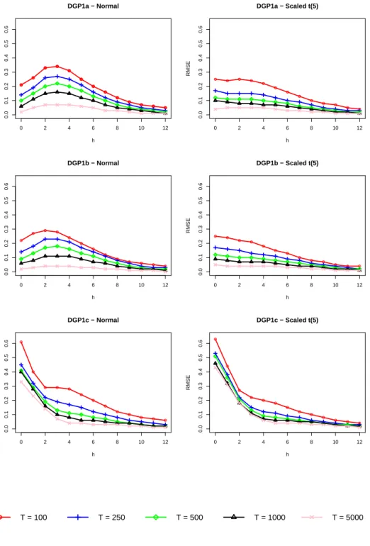
The importance of the finite fourth moment assumption for the consistency of the structural impulse response estimator (13) is analyzed by means of a simulation-based root mean squared error (RMSE) analysis. More specifically, three different data generating processes (DGPs) are considered from which two DGPs satisfy all assumptions required for consistency (DGP-1a and DGP-1b) and one DGP that violates the finite fourth moment assumption (DGP-1c); see Section5.1for more details. The results forΘb11,h, h∈ {0, . . . ,12}, are found in Appendix D.
The analysis highlights the importance of the assumption ofE[ε4t,i]<+∞. For the two DGPs withE[ε4t,i]<+∞, the RMSE of the structural impulse response estimator is strictly decreasing in the sample size and, for very large sample sizes, close to zero at all propagation horizons h. In contrast, for the DGP that violates the assumptionE[ε4t,i]<+∞, the RMSE of the estimator is only weakly decreasing. Moreover, for small propagation horizonsh∈ {0,1,2,3}, the RMSE is substantially away from zero even for a very large sample size ofT = 5,000.
3
Inference for Structural Impulse Responses
3.1 Motivation
We are interested in constructing a marginal bootstrap percentile confidence interval `a la Hall
percentile confidence interval for Θij,h with a nominal coverage probability of (1−α)∈(0,1) is given by CIh,(1−α)..= h b Θij,h−q∗h,(1−α/2);Θbij,h−qh,α/∗ 2 i , (15)
whereq∗h,(1−α/2) andq∗h,(α/2)are the (1−α/2)- and (α/2)-quantiles, respectively, of the bootstrap sampling distribution (at propagation horizonh). Evidently, the confidence interval CIh,(1−α)
is derived under the usual bootstrap analogy, that is, the bootstrap sampling distribution approximates the unknown true sampling distribution
LΘb∗ij,h−Θbij,h |y−p+1, . . . , y0, y1, . . . , yT
≈ LΘbij,h−Θij,h
, (16)
where L(X) denotes the distribution of a random variable X and Θb∗ij,h denotes the estimator
computed based on artificial bootstrap data y−p∗ +1, . . . , y∗0, y∗1, . . . , y∗T . Hence, a bootstrap procedure that satisfies (16) is expected to produce a confidence interval CIh,(1−α) that exhibits
an actual coverage probability that is close to the nominal coverage probability (1−α), and therefore provides valid inference.
The deviation from i.i.d. reduced-form errors by specifying the reduced-form error process as a conditionally heteroskedastic GO-GARCH model (see Section2.2) entails that standard bootstrap procedures, such as the procedures of Runkle (1987), Kilian (1998a) and Kilian
(1998b), may not result in a valid percentile confidence interval for Θij,h, even for very large sample sizes. The reason being that these bootstrap procedures are based on resampling with replacement from the empirical distribution of the reduced-form residuals, and hence the validity of these procedures essentially relies on the underlying assumption of i.i.d. reduced-form errors.
Br¨uggemann et al.(2016) investigate, among other things, inference for structural impulse responses in VAR models with conditional heteroskedasticity of unknown form and propose a residual-based moving block bootstrap procedure in the spirit ofK¨unsch(1989). However, the authors prove the validity of their proposed moving block bootstrap only for structural impulse responses which are identified via a standard recursive ordering approach6; see Corollary 5.2 of Br¨uggemann et al. (2016, p.75). Thus, their theoretical result does not directly apply to structural impulse responses that are identified via the conditional heteroskedasticity of the GO-GARCH model. The same concern applies to the results of the extensive Monte Carlo study ofBr¨uggemann et al. (2016). Moreover, we are not aware of a study that provides theoretical or simulation-based results that are applicable in the present framework where the structural impulse responses are identified via the conditional heteroskedasticity in the error process.
We propose a nonparametric bootstrap procedure that explicitly incorporates the GO-GARCH structure of the reduced-form error process. In this way, the corresponding artificial bootstrap data resembles the data generated from the true model, and hence the resulting bootstrap sampling distribution is supposed to approximate the true sampling distribution, at least for large sample sizes. Moreover, the proposed bootstrap procedure can be viewed as
6
a multivariate generalization of the bootstrap procedure for the univariate ARMA-GARCH model outlined inShimizu (2010, p.68–70).
The proposed bootstrap procedure is straightforward to implement, as it only requires the availability of the following quantities: (i) the estimators of the model parameters, that is, ˆ
ν,Aˆ1, . . . ,Ap,ˆ B˘ˆ0−1,αˆ˘ and
ˆ ˘
β; (ii) the corresponding series of residuals{uˆ1, . . . ,uTˆ }; and (iii) the
pre-sample of the original data{y−p+1, . . . , y0}.
3.2 Residual Bootstrap
The following bootstrap algorithm, subsequently referred to as the residual bootstrap, produces the marginal percentile interval at each propagation horizonh∈ {0, . . . , H}.
a) For each componenti= 1, . . . , m, compute the estimated conditional variances according to
ˆ
σ2t,i ..= (1−αiˆ˘ −βi) + ˆ˘ˆ αi˘ εˆ2t−1,i+ ˆ ˘
βiσˆt−2 1,i, t= 1, . . . , T ,
where the starting values are ˆε20,i ..= ˆσ2
0,i = (1−αˆ˘i −βˆ˘i). Next, obtain the estimated conditional variance matrices ˆHt..= diag(ˆσt,21, . . . ,ˆσ2t,m),t= 1, . . . , T.
b) Compute the devolatized residuals ˆet ..= ˆHt−1/2Bˆ˘0ut,ˆ t = 1, . . . , T. Next, center and rescale the devolatized residuals according to
˘ et..= ˆΣe−1/2 ˆet−e¯ˆ , t= 1, . . . , T , where ¯eˆ..=T−1PT t=1ˆet and ˆΣe..=T −1PT t=1(ˆet−e)(ˆ¯ˆ et−¯ˆe) 0.
c) For each componenti= 1, . . . , m, generate the univariate bootstrap sample
n ˆ ε∗1,i, . . . ,εˆ∗T ,i o according to ˆ ε∗t,i..= ˆσ∗ t,iˆe∗t,i ˆ σt,i∗2..= (1−αˆ˘i−β˘ˆi) + ˆα˘iεˆ∗t−21,i+βˆ˘iσˆt−∗21,i ,
where ˆe∗t,i is a random draw with replacement from the (univariate) empirical distribution of{et,i˘ }Tt=1. The starting values are ˆε∗02,i..= ˆσ0∗,i2 = (1−αiˆ˘ −βi). Next, obtain the series ofˆ˘ bootstrap residuals{uˆ∗1, . . . ,uˆ∗T} via u∗t ..=Bˆ˘−1
0 εˆ∗t,t= 1, . . . , T. d) Generate the bootstrap sample{y∗1, . . . , y∗T}according to
yt∗..= ˆν+ ˆA1y∗
t−1+. . .+ ˆApy∗t−p+u∗t , t= 1, . . . , T ,
e) Compute the estimators ˆν∗,Aˆ∗1, . . . ,Aˆ∗p and ˆB0−1∗ based on y∗−p+1, . . . , y0∗, y1∗, . . . , yT∗ . Replace ˆB0−1∗ with an equivalent matrix Bˆ˘0−1∗ which satisfies
ˆ ˘ B0−1∗ ∈ arg min B∈E( ˆB−01∗) B− ˆ ˘ B0−1 F ,
wherek·kF denotes the Frobenius norm; see Remark 3.1 for a comment. Next, compute the bootstrap impulse responseΘb∗ij,h..=fij,h
ˆ
A1∗, . . . ,Aˆ∗p,Bˆ˘0−1∗.
f) Repeat steps b) to d)B times and obtain the empirical bootstrap sampling distribution
n b
Θ∗ij,h,b−Θbij,h oB
b=1 for each propagation horizonh
∈ {0, . . . , H}. Determine the marginal percentile intervals by h b Θij,h−q˜∗h,(1−α/2);Θbij,h−q˜h,α/∗ 2 i ,
where ˜qh,∗(1−α/2) and ˜q∗h,α/2 are the empirical (1−α/2)- and (α/2)-quantiles, respectively, of n b Θ∗ij,h,b−Θij,hb oB b=1.
Remark 3.1. The replacement of ˆB0−1∗ with Bˆ˘0−1∗ in step e) of the residual bootstrap ensures that the bootstrap structural impulse response estimator Θb∗ij,h is computed based on the
particular matrix B˘ˆ0−1∗ ∈ E( ˆB0−1∗) that is closest to the matrix Bˆ˘−01 which is at the basis of the structural impulse response estimator Θij,h. In this way, the particular bootstrapb
VMA representation (characterized by Bˆ˘0−1∗) is selected that is most similar to the VMA representation characterized byBˆ˘−01.
We also consider a modified version of the residual bootstrap procedure. The modified version, subsequently referred to as the symmetrized residual bootstrap, is obtained by the following modification in step c): ˆe∗t,i is a random draw with replacement from the empirical distribution of thesymmetrized series {e˜1,i, . . . ,˜e2T ,i}..={±e˘1,i, . . . ,±˘eT ,i}of length 2T instead of the empirical distribution of {˘e1,i, . . . ,˘eT,i} as in the residual bootstrap; see AppendixCfor details.
The modification serves the purpose to ensure that the empirical skewness of{e˜1,i, . . . ,e˜2T ,i} is zero. Furthermore, note that the first and the second empirical moment of{e˜1,i, . . . ,e˜2T ,i} is equal to zero and one, respectively, due to the preceding centering and rescaling in step b). Thus, in scenarios where the true distribution ofet,i is symmetric around zero (e.g. et,i ∼ N(0,1)), and hence exhibits a skewness of zero7, the empirical distribution of {e˜1,i, . . . ,e˜2T ,i} matches not only the first and the second moment but also the skewness of the true distribution ofet,i. Eventually, this modification results in improved finite-sample properties of the corresponding confidence intervals in these scenarios.
7Here, we tacitly assume that
4
Competing Methods
In order to assess the finite-sample performance of the residual bootstrap and the symmetrized residual bootstrap, we compare their finite-sample properties with two competing procedures: (i) the standard i.i.d. bootstrap originally proposed byRunkle(1987) and (ii) the moving-block bootstrap proposed inBr¨uggemann et al.(2016). In the following, the two competing procedures are briefly outlined.
4.1 I.i.d. Bootstrap
a) Generate the bootstrap sample{y∗1, . . . , y∗T}according to yt∗..= ˆν+ ˆA1y∗
t−1+. . .+ ˆApy∗t−p+ ˜u∗t , t= 1, . . . , T ,
where ˜u∗t is a random draw with replacement from the empirical distribution of the centered and rescaled (reduced-form) residuals8. The starting values are equal to the pre-sample of the original series{y−p+1, . . . , y0}.
b) identical to step e) of the residual bootstrap. c) identical to step f) of the residual bootstrap. 4.2 Moving-Block Bootstrap
a) Choose a block length l < T and let N ..= dT /le denote the number of blocks. Define Bi,l ..= (ˆui+1, . . . ,uiˆ+l), i = 0, . . . , T −l and let i1, . . . , iN be i.i.d. random variables
uniformly distributed on the set{0,1, . . . , T −l}. Obtain {uˆ∗1, . . . ,uˆ∗T} by laying blocks Bi1,l, . . . , BiN,l end-to-end together and discard the last N l−T observations.
b) Center {uˆ∗1, . . . ,uˆ∗T} according to ˘ u∗jl+s ..= ˆu∗ jl+s− 1 T−l+ 1 T−l X r=0 ˆ us+r , t= 1, . . . , T , (17) fors= 1,2, . . . , l and j= 0,1,2, . . . , N−1.
c) Generate the bootstrap sample{y∗1, . . . , y∗T}according to yt∗..= ˆν+ ˆA1y∗
t−1+. . .+ ˆApy∗t−p+ ˘u∗t , t= 1, . . . , T ,
where the starting values are equal to the pre-sample of the original series{y−p+1, . . . , y0}.
d) identical to step e) of the residual bootstrap. e) identical to step f) of the residual bootstrap.
In the Monte Carlo simulations, the block lengths are given by l ∈ {10,20,50,75,200} for sample sizes T ∈ {100,250,500,1000,5000}. ForT ∈ {500,5000}, the block lengths are as in
Br¨uggemann et al.(2016). The sample sizes T ∈ {100,250,1000} are not considered in their study, and hence the block lengths are found via interpolation.
5
Monte Carlo Simulation
5.1 Data Generating Processes
We consider the following bivariate model fromBr¨uggemann et al.(2016), that is,
DGP-1 yt=A1yt−1+A2yt−2+B0−1εt , (18) where A1 ..= 0.40 0.60 −0.10 1.20 ! , A2..= −0.20 0.00 −0.20 −0.10 ! and B0−1..= 1.00 0.00 0.50 √0.75 ! .
The moduli of the roots of the characteristic polynomial of the VAR are given by 1.08, 2.78, and 5.98, which implies moderate persistence of the process{yt:t∈Z}. The following set of different GARCH(1,1) specifications for the two components of {εt:t∈Z} are considered
a) (α1, β1)0= (0.10,0.80)0; (α2, β2)0 = (0.20,0.65)0,
b) (α1, β1)0= (0.10,0.80)0; (α2, β2)0 = (0.085,0.90)0,
c) (α1, β1)0= (0.095,0.90)0; (α2, β2)0= (0.25,0.65)0,
where the specific variants of DGP-1 will be denoted by DGP-1i,i∈ {a, b, c}, depending on the specific choice of the GARCH specification.
The following two univariate distributions for the (mutually independent) components of the i.i.d. process{et:t∈Z}are considered:
• et,i ∼ N(0,1), standard normal distribution.
• et,i ∼ 35t5,t-distribution with 5 degrees of freedom, scaled to have variance 1.
Under DGP-1a, the persistence of the GARCH processes, measured by αi+βi, is given by 0.90 and 0.85, respectively which implies only moderate persistence. For both considered distributions of et,i, DGP1a implies a consistent estimator Θbij,h of the structural impulse
responses. Under DGP-1b, the persistence is given by 0.90 and 0.985, respectively. Similarly to DGP-1a, DGP-1b implies a consistent estimatorΘij,hb for both distributions of et,i. Under
DGP-1c, the persistence of the GARCH processes is given by 0.995 and 0.90, respectively. The first component of εt does not have a finite fourth moment (for both distributions ofet,i) and hence the assumptions underlying the consistency of Θij,hb are violated. Hence, this DGP is
included to investigate the sensitivity of the bootstrap procedure from deviations of the finite fourth moment assumption.
5.2 Simulation Parameters and Performance Evaluation
Data samples of length T ∈ {100,250,500,1000,5000} are generated and the maximum propagation horizon is H = 12. The nominal confidence level of the marginal confidence bands is 90%. The number of bootstrap replications isB = 1000 throughout and the number of Monte Carlo replications is 1000. The finite-sample performance of the confidence intervals is evaluated by the empirical coverage rate and the empirical length. In particular, the empirical empirical coverage rate is computed in the usual way as
ECij,h ..= 1 1000 1000 X m=1 1{Θij,h∈ CIij,h,m} ,
where CIij,h denotes the marginal confidence interval for Θij,h and1{A} denotes the indicator function of an eventA. The empirical length is computed as
Lij,h..= 1 1000 1000 X m=1 (uij,h,m−lij,h,m) ,
whereuij,h,m denotes the upper bound of the marginal confidence interval for Θij,h and lij,h,m denotes the corresponding lower bound.
5.3 Results
The boxplots summarizing the performance of the four different bootstrap methods across different scenarios are found in AppendicesE, Fand G. The tables with the simulation results (empirical coverage rates and empirical lengths) are available from the authors upon request. The main conclusions are as follows:
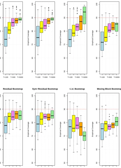
• Under DGP-1a with et,i ∼ N(0,1) and T = 100, the empirical coverage rates of the confidence intervals based on the residual bootstrap exhibit a large dispersion among propagation horizons h and impulse responses ranging from 63.60% to 96.90%. Yet, increasing the sample sizeT results in a substantial reduction in the coverage bias and its dispersion. ForT = 5000, the range of the coverage rates of the confidence intervals is given by 86.90% to 96.00%. Heavy-tailed GARCH errors, that is,et,i∼ 35t5, increase the
coverage bias of the residual bootstrap especially forT ∈ {1000,5000}.
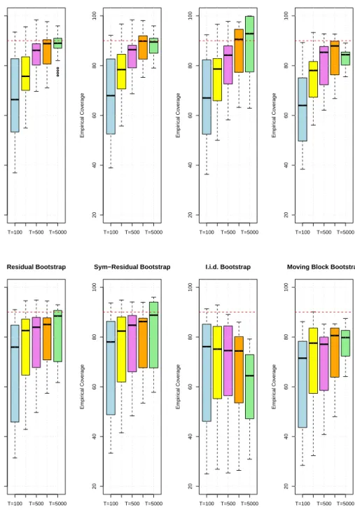
The higher persistence in the GARCH process ofεt,2 in DGP-1bhas an overall negative
effect on the coverages rates of the intervals based on the residual bootstrap, but the negative effect is more pronounced for impulse responses where the shock occurs in the second variable, that is, Θ12,h and Θ22,h. For T = 100 and et,i ∼ N(0,1), the coverage
rates range from 36.90% to 93.50%. The negative coverage bias of the residual bootstrap is decreasing in the sample size T but even with T = 5000 the range of the coverage rates is 77.10% to 96.40%. The heavy-tailed GARCH errors (et,i ∼ 35t5) result in larger
coverage biases for all sample sizes, where the negative effect is more pronounced than under the less persistent DGP-1a.
The non-finite fourth moment of εt,1 in DGP-1c has also an overall negative effect on
the coverage rates of the residual bootstrap. The strongest effect is on the intervals for Θ11,0 and Θ11,1. ForT = 100 and et,i ∼ N(0,1), the coverage rates for Θ11,0 and Θ11,1
are 4.40% and 27.80%, respectively, whereas the remaining coverage rates range from 61.00% to 95.30%. The effect of an increase in the sample size T is ambiguous; increasing the sample size toT ∈ {250,500}results in a overall reduction of the coverage bias of the confidence intervals, but after that, a further increase toT ∈ {1000,5000} results either in nearly no improvement or even in a deterioration of the performance (compared to the T = 500 scenario). Similarly to DGP-1aand DGP-1b, heavy-tailed GARCH errors result in an increase in the coverage bias.
• Overall, the symmetrized residual bootstrap exhibits a very similar performance as the residual bootstrap. Hence, the symmetrized residual bootstrap is not capable of systematically outperforming the residual bootstrap, although both considered distributions ofet,i are symmetric around zero.
• Under DGP-1a with et,i ∼ N(0,1) and T = 100, similar to the residual bootstrap, the empirical coverage rates of the confidence intervals based on the i.i.d. bootstrap exhibit a large dispersion among propagation horizons h and impulse responses ranging from 63.40% to 96.70%. Increasing the sample size T results in higher empirical coverage rates of the intervals based on the i.i.d. bootstrap. For T = 5000, the coverages rates range between 79.80% and 99.30%, however, the majority of confidence intervals exhibit coverages rates above the nominal level of 90%. The effect of heavy-tailed GARCH errors is drastic; the confidence intervals for 42 (out of 52) impulse responses exhibit a lower coverage rate with T = 5000 than with T = 100.
Under DGP-1b, the performance of the i.i.d. bootstrap is basically similar to DGP-1a except that the dispersion of the coverage rates among the propagation horizons and the structural impulse responses is more pronounced. For T = 100 and et,i ∼ N(0,1), the coverage rates range between 36.30% and 92.40% and withT = 5000, the range is still given by 62.90% to 100.00%. The effect of heavy-tailed GARCH errors is again disastrous. Even for the very large sample sizeT = 5000, the coverage rates of the intervals based on the i.i.d bootstrap vary between 32.00% and 79.20%.
The violation of the finite fourth moment assumption (DGP-1c) exhibits an overall negative effect on the confidence intervals based on the i.i.d. bootstrap. Similar to the residual bootstrap, the intervals for Θ11,0 and Θ11,1 are the most affected with coverage
rates of 3.3% and 30.50% forT = 100 andet,i∼ N(0,1). Moreover, the behavior of the coverage rates depending on the sample size is erratic; for some impulse responses the coverage rate of the corresponding interval is increasing in the sample size and for others the coverage rate is indeed decreasing in the sample size. Heavy-tailed GARCH errors result in an overall performance that is decreasing with the sample sizeT.
• Under DGP-1a with et,i ∼ N(0,1) and T = 100, the empirical coverage rates of the confidence intervals based on the moving block bootstrap also exhibit a large dispersion among propagation horizons h and impulse responses ranging from 61.00% to 92.00%. The overall coverage bias is decreasing for sample sizesT ∈ {250,500,1000} but a further increase toT = 5000 exhibits an ambiguous effect on the coverage rates of the moving block bootstrap. For T = 5000, the range of the coverage rates is given by 76.70% to 89.90%. Heavy-tailed GARCH errors result in a downward shift of the coverage rates of the confidence intervals based on the moving block bootstrap; forT = 5000, the coverage rates vary between 70.00% and 87.00%.
The higher persistence of DGP-1bresults in higher coverage biases and more dispersion. For T = 100 and et,i∼ N(0,1), the coverage rates of the intervals based on the moving-block bootstrap are between 38.40% and 89.30%. Similar to DGP-1a, the overall performance continuously improves only for T ∈ {250,500,1000}. For T = 5000, the coverage rates range between 75.50% and 89.10%. Heavy-tailed GARCH errors increase the bias and the dispersion of the intervals based on the moving block bootstrap.
Under DGP-1c, the violation of the finite fourth moment assumption exhibits an overall negative effect on the intervals based on the moving block bootstrap. Similar to the residual and the i.i.d. bootstrap, the intervals for Θ11,0 and Θ11,1 are the most affected
with coverage rates of 2.70% and 26.20%, respectively for T = 100 andet,i ∼ N(0,1). The effect of an increasing sample size is ambiguous and depends on the particular impulse response under consideration. ForT = 5000, the range of the coverage rates is 51.10% to 87.90%. Again, the heavy-tailed GARCH errors result in a deterioration of the performance of the confidence intervals based on the moving block bootstrap.
• The confidence intervals based on the residual bootstrap exhibits the smallest absolute deviation from the nominal level in 1188 out of the 1560 scenarios. The intervals based on the i.i.d. bootstrap and the moving block bootstrap exhibit the smallest absolute deviation in only 199/1560 and 173/1560 scenarios, respectively9. Hence, the residual
bootstrap exhibits the best overall performance in terms of the coverage bias.
• For the small sample sizeT = 100, neither of the bootstrap methods is capable of reliably producing a bootstrap sampling distribution that constitutes a good approximation of the true sampling distribution. Hence, the resulting confidence intervals eventually understate the actual estimation uncertainty; see Appendix H for an analysis of the bootstrap sampling distributions as a function of the sample size.
• The results of the Monte Carlo simulations confirm the result fromBr¨uggemann et al.
(2016) that the presence of heteroskedasticity substantially increases the estimation uncertainty.
9
The symmetrized residual bootstrap is omitted in this comparison because it is a modification of the residual bootstrap.
6
Conclusion
A recent strand of the literature exploits conditional heteroskedasticity to identify the structural vector autoregressions. However, the implications for inference on structural impulse responses have not been investigated in the literature yet.
In this paper, we have considered the conditionally heteroskedastic SVAR-GARCH model. We have proposed (i) an estimation procedure of the model parameters that offers numerical stability even in small sample and/or high dimension scenarios and (ii) a bootstrap procedure to construct marginal percentile confidence intervals for structural impulse responses.
By means of a Monte Carlo simulation, we have compared the finite-sample properties of our proposed bootstrap method to those of two benchmarking methods: the i.i.d. bootstrap of
Runkle(1987) and the moving block bootstrap ofBr¨uggemann et al.(2016). The confidence intervals based on our proposed bootstrap method exhibits the best overall performance. Nevertheless, the intervals may understate the estimation uncertainty by a substantial amount especially in small samples.
References
Bollerslev, T. (1986). Generalized autoregressive conditional heteroskedasticity. Journal of Econometrics, 31(3):307–327.
Boswijk, H. P. and van der Weide, R. (2011). Method of moments estimation of GO-GARCH models. Journal of Econometrics, 163(1):118–126.
Bouakez, H., Chihi, F., and Normandin, M. (2014). Measuring the effects of fiscal policy.
Journal of Economic Dynamics and Control, 47:123–151.
Bouakez, H., Essid, B., and Normandin, M. (2013). Stock returns and monetary policy: Are there any ties? Journal of Macroeconomics, 36:33–50.
Bouakez, H. and Normandin, M. (2010). Fluctuations in the foreign exchange market: How important are monetary policy shocks? Journal of International Economics, 81(1):139–153. Boussama, F., Fuchs, F., and Stelzer, R. (2011). Stationarity and geometric ergodicity of BEKK multivariate GARCH models. Stochastic Processes and their Applications, 121(10):2331 – 2360.
Br¨uggemann, R., Jentsch, C., and Trenkler, C. (2016). Inference in VARs with conditional heteroskedasticity of unknown form. Journal of Econometrics, 191(1):69–85.
Engle, R. F. and Kroner, K. F. (1995). Multivariate simultaneous generalized ARCH.
Econometric Theory, 11(1):122–150.
Flury, B. N. and Gautschi, W. (1986). An algorithm for simultaneous orthogonal transformation of several positive definite symmetric matrices to nearly diagonal form. SIAM Journal on Scientific and Statistical Computing, 7(1):169–184.
Francq, C. and Ra¨ıssi, H. (2007). Multivariate Portmanteau test for autoregressive models with uncorrelated but nonindependent errors. Journal of Time Series Analysis, 28(3):454–470. Hall, P. (1992). The Bootstrap and Edgeworth Expansion. Springer, New York.
He, C. and Ter¨asvirta, T. (1999). Fourth moment structure of the GARCH(p, q) process.
Econometric Theory, 15(6):824–846.
Herwartz, H. and L¨utkepohl, H. (2014). Structural vector autoregressions with markov switching: Combining conventional with statistical identification of shocks. Journal of Econometrics, 183(1):104–116.
Hill, J. B. (2015). Robust estimation and inference for heavy tailed GARCH. Bernoulli, 21(3):1629–1669.
Hwang, S. and Pereira, P. L. V. (2006). Small sample properties of GARCH estimates and persistence. European Journal of Finance, 12(6-7):473–494.
Kilian, L. (1998a). Accounting for lag order uncertainty in autoregressions: the endogenous lag order bootstrap algorithm. Journal of Time Series Analysis, 19(5):531–548.
Kilian, L. (1998b). Small-sample confidence intervals for impulse response functions. Review of Economics and Statistics, 80(2):218–230.
Kilian, L. (2013). Structural vector autoregressions. In Handbook of Research Methods and Applications in Empirical Macroeconomics, chapter 22, pages 515–554. Edward Elgar Publishing.
Kilian, L. and L¨utkepohl, H. (2017). Structural Vector Autoregressive Analysis. Themes in Modern Econometrics. Cambridge University Press.
Kristensen, D. and Linton, O. (2006). A closed-form estimator for the GARCH(1,1) model.
Econometric Theory, 22(2):323337.
K¨unsch, H. R. (1989). The jackknife and the bootstrap for general stationary observations.
Annals of Statistics, 17(3):1217–1241.
Lanne, M., L¨utkepohl, H., and Maciejowska, K. (2010). Structural vector autoregressions with markov switching. Journal of Economic Dynamics and Control, 34(2):121–131.
Lanne, M. and Saikkonen, P. (2007). A multivariate generalized orthogonal factor GARCH model. Journal of Business & Economic Statistics, 25(1):61–75.
L¨utkepohl, H. (2005). New Introduction to Multiple Time Series Analysis. Springer, Berlin. L¨utkepohl, H. and Milunovich, G. (2016). Testing for identification in SVAR-GARCH models.
Journal of Economic Dynamics and Control, 73:241 – 258.
L¨utkepohl, H. and Netˇsunajev, A. (2017). Structural vector autoregressions with heteroskedas-ticity: A review of different volatility models. Econometrics and Statistics, 1:2 – 18.
Milunovich, G. (2014). Complete and partial identification of the A-and B-models in the context of heteroskedastic SVARs. Available at SSRN: http://ssrn.com/abstract=2484300. Normandin, M. and Phaneuf, L. (2004). Monetary policy shocks: Testing identification
conditions under time-varying conditional volatility. Journal of Monetary Economics, 51(6):1217–1243.
Preminger, A. and Storti, G. (2017). Least-squares estimation of GARCH(1,1) models with heavy-tailed errors. Econometrics Journal, 20(2):221–258.
Runkle, D. E. (1987). Vector autoregressions and reality. Journal of Business & Economic Statistics, 5(4):437–442.
Shimizu, K. (2010). Bootstrapping Stationary ARMA-GARCH Models. Springer, Berlin. Stine, R. A. (1987). Estimating properties of autoregressive forecasts. Journal of the American
Statistical Association, 82(400):1072–1078.
van der Weide, R. (2002). GO-GARCH: A multivariate generalized orthogonal GARCH model.
A
Method-of-Moment Estimator of GO-GARCH Models
The following algorithm describes the computation of the method of moment estimator ˆB−01 outlined inBoswijk and van der Weide (2011) based on the series of reduced-form residuals
{uˆ1, . . . ,uˆT}.
1. Based on{uˆ1, . . . ,uTˆ }, estimate the unconditional variance matrixΣub ..=T−1 PT
t=1utˆ uˆ
0 t and obtain its symmetric square root ˆS. Next, compute the standardized seriesst..= ˆS−1uˆt, t= 1, . . . , T.
2. Obtain the matrix-valued series St ..= sts0t −Im, t = 1, . . . , T, and the sample auto-covariance matrices ˆΓ(k) ..= T−1PT
t=1StSt−k, k = 1, . . . ,˜k. Next, obtain the sample
auto-correlation matrices ˆ
Φ(k)..= ˆΓ(0)−1/2Γ(k)ˆˆ Γ(0)−1/2 , k= 1, . . . ,˜k ,
where ˆΓ(0)−1/2denotes the symmetric square root of ˆΓ(0)−1. Next, obtain the symmetrized sample auto-correlation matrices ˜Φ(k)..= 1
2( ˆΦ(k) + ˆΦ(k)
0),k= 1, . . . ,k.˜
3. The estimator ˆU is then obtained by minimizing the following objective function
S(U)..= ˜
k
X
k=1
trU0Φ(k)U˜ −diag(U0Φ(k)U˜ )0×trU0Φ(k)U˜ −diag(U0Φ(k)U˜ ) ,
over all orthogonal matricesU, where tr(·) denotes the trace operator. The solution to the minimization problem is obtained via the F-G algorithm ofFlury and Gautschi(1986). 4. Compute the estimator ˆB0−1..= ˆSUˆ.
B
Least-Squares Estimator of Univariate GARCH(1,1) Models
The following algorithm describes the computation of the least-squares estimator ( ˆαi,βi)ˆ 0 outlined in Preminger and Storti (2017) of the i-th GARCH process based on the series of structural errors{εˆ1,i, . . . ,εT ,iˆ }.
1. Using the univariate series{εˆ1,i, . . . ,εˆT ,i}, estimate the GARCH parameters (αi, βi)0 via the quasi-maximum tail-trimmed likelihood (QMTTL) estimator of Hill(2015, p.7); see RemarkB.1. Obtain the corresponding devolatized residuals ˆet,i ..= ˆε1,i/ˆσt,i, t= 1, . . . , T,
where ˆσt,i denotes the estimate based on the QMTTL estimator. Next, compute
ˆ cT ..= 1 T T X t=1 log ˆe2t,i .
2. The least-squares estimator ( ˆαi,βi) ofˆ Preminger and Storti(2017) is then obtained by minimizing the following objective function
QT( ˜α,β˜; ˆcT)..= 1 T T X t=1
log(ˆε2t,i)−cTˆ −log(ˆσ2t,i( ˜α,β))˜
2
,
that is, ( ˆαi,βˆi)..= arg min
( ˜α,β˜)0∈Θ
QT( ˜α,β; ˆ˜ cT).
Remark B.1. Preminger and Storti (2017) use the standard quasi-maximum likelihood estimator ( ˆαQMLi ,βˆiQML)0 in the first step instead of the QMTTL estimator of Hill (2015). We replaced the standard QML estimator with the QMTTL estimator ofHill(2015) because the aforementioned estimator enjoys improved convergence properties in small samples compared to the standard QML estimator.
C
Symmetrized Residual Bootstrap
a) identical to the residual bootstrap. b) identical to the residual bootstrap.
c) For each componenti= 1, . . . , m, generate the univariate bootstrap sample
n ˆ ε∗1,i, . . . ,εˆ∗T ,i o according to ˆ
ε∗t,i = ˆσ∗t,ieˆ∗t,i ˆ
σ∗t,i2= (1−αˆ˘i−β˘ˆi) + ˆα˘iεˆ∗t−21,i+ ˆ ˘
βiσˆt−∗21,i ,
where ˆe∗t,i is a random draw with replacement from the univariate empirical distribution of the symmetrized series{˜e1,i, . . . ,˜e2T,i}..={±˘e1,i, . . . ,±e˘T ,i}of length 2T. The starting values are ˆε∗02,i = ˆσ0∗2,i = (1−αiˆ˘ −βi). Next, obtain the series of bootstrap residualsˆ˘
{uˆ∗1, . . . ,uˆ∗T} viau∗t =Bˆ˘0−1εˆ∗t,t= 1, . . . , T. d) identical to the residual bootstrap.
e) identical to the residual bootstrap. f) identical to the residual bootstrap.
D
RMSE
0 2 4 6 8 10 12 0.0 0.1 0.2 0.3 0.4 0.5 0.6 DGP1a − Normal h RMSE 0 2 4 6 8 10 12 0.0 0.1 0.2 0.3 0.4 0.5 0.6 DGP1a − Scaled t(5) h RMSE 0 2 4 6 8 10 12 0.0 0.1 0.2 0.3 0.4 0.5 0.6 DGP1b − Normal h RMSE 0 2 4 6 8 10 12 0.0 0.1 0.2 0.3 0.4 0.5 0.6 DGP1b − Scaled t(5) h RMSE 0 2 4 6 8 10 12 0.0 0.1 0.2 0.3 0.4 0.5 0.6 DGP1c − Normal h RMSE 0 2 4 6 8 10 12 0.0 0.1 0.2 0.3 0.4 0.5 0.6 DGP1c − Scaled t(5) h RMSE T = 100 T = 250 T = 500 T = 1000 T = 5000Figure D.1: Root mean squared error (RMSE) ofΘb11,h for propagation horizonsh∈ {0, . . . ,12}
E
DGP-1a
T=100 T=500 T=5000 50 60 70 80 90 100 Residual Bootstrap Empir ical Co v er age T=100 T=500 T=5000 50 60 70 80 90 100 Sym−Residual Bootstrap Empir ical Co v er age T=100 T=500 T=5000 50 60 70 80 90 100 I.i.d. Bootstrap Empir ical Co v er age T=100 T=500 T=5000 50 60 70 80 90 100Moving Block Bootstrap
Empir ical Co v er age T=100 T=500 T=5000 50 60 70 80 90 100 Residual Bootstrap Empir ical Co v er age T=100 T=500 T=5000 50 60 70 80 90 100 Sym−Residual Bootstrap Empir ical Co v er age T=100 T=500 T=5000 50 60 70 80 90 100 I.i.d. Bootstrap Empir ical Co v er age T=100 T=500 T=5000 50 60 70 80 90 100
Moving Block Bootstrap
Empir
ical Co
v
er
age
Figure E.1: Boxplots of the empirical coverages across all impulse responses and all propagation horizons (52 parameter constellations in total) of nominal 90% marginal confidence intervals for T ∈ {100,250,500,1000,5000}. The first row corresponds to et,i
i.i.d.
∼ N(0,1) and the second row corresponds toet,ii.i.d.∼ 35t5.
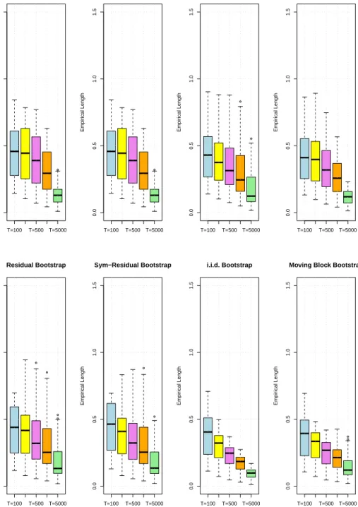
T=100 T=500 T=5000 0.0 0.5 1.0 1.5 Residual Bootstrap Empir ical Length T=100 T=500 T=5000 0.0 0.5 1.0 1.5 Sym−Residual Bootstrap Empir ical Length T=100 T=500 T=5000 0.0 0.5 1.0 1.5 I.i.d. Bootstrap Empir ical Length T=100 T=500 T=5000 0.0 0.5 1.0 1.5
Moving Block Bootstrap
Empir ical Length T=100 T=500 T=5000 0.0 0.5 1.0 1.5 Residual Bootstrap Empir ical Length T=100 T=500 T=5000 0.0 0.5 1.0 1.5 Sym−Residual Bootstrap Empir ical Length T=100 T=500 T=5000 0.0 0.5 1.0 1.5 I.i.d. Bootstrap Empir ical Length T=100 T=500 T=5000 0.0 0.5 1.0 1.5
Moving Block Bootstrap
Empir
ical Length
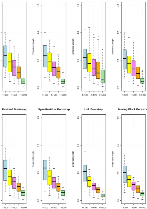
Figure E.2: Boxplots of the empirical lengths across all impulse responses and all propagation horizons (52 parameter constellations in total) of nominal 90% marginal confidence intervals for T ∈ {100,250,500,1000,5000}. The first row corresponds to et,i i.i.d.∼ N(0,1) and the second row corresponds toet,i
i.i.d.
∼ 3 5t5.
F
DGP-1b
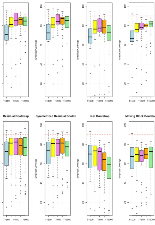
T=100 T=500 T=5000 20 40 60 80 100 Residual Bootstrap Empir ical Co v er age T=100 T=500 T=5000 20 40 60 80 100 Sym−Residual Bootstrap Empir ical Co v er age T=100 T=500 T=5000 20 40 60 80 100 I.i.d. Bootstrap Empir ical Co v er age T=100 T=500 T=5000 20 40 60 80 100Moving Block Bootstrap
Empir ical Co v er age T=100 T=500 T=5000 20 40 60 80 100 Residual Bootstrap Empir ical Co v er age T=100 T=500 T=5000 20 40 60 80 100 Sym−Residual Bootstrap Empir ical Co v er age T=100 T=500 T=5000 20 40 60 80 100 I.i.d. Bootstrap Empir ical Co v er age T=100 T=500 T=5000 20 40 60 80 100
Moving Block Bootstrap
Empir
ical Co
v
er
age
Figure F.1: Boxplots of the empirical coverages across all impulse responses and all propagation horizons (52 parameter constellations in total) of nominal 90% marginal confidence intervals for T ∈ {100,250,500,1000,5000}. The first row corresponds to et,i
i.i.d.
∼ N(0,1) and the second row corresponds toet,ii.i.d.∼ 35t5.
T=100 T=500 T=5000 0.0 0.5 1.0 1.5 Residual Bootstrap Empir ical Length T=100 T=500 T=5000 0.0 0.5 1.0 1.5 Sym−Residual Bootstrap Empir ical Length T=100 T=500 T=5000 0.0 0.5 1.0 1.5 i.i.d. Bootstrap Empir ical Length T=100 T=500 T=5000 0.0 0.5 1.0 1.5
Moving Block Bootstrap
Empir ical Length T=100 T=500 T=5000 0.0 0.5 1.0 1.5 Residual Bootstrap Empir ical Length T=100 T=500 T=5000 0.0 0.5 1.0 1.5 Sym−Residual Bootstrap Empir ical Length T=100 T=500 T=5000 0.0 0.5 1.0 1.5 i.i.d. Bootstrap Empir ical Length T=100 T=500 T=5000 0.0 0.5 1.0 1.5
Moving Block Bootstrap
Empir
ical Length
Figure F.2: Boxplots of the empirical lengths across all impulse responses and all propagation horizons (52 parameter constellations in total) of nominal 90% marginal confidence intervals for T ∈ {100,250,500,1000,5000}. The first row corresponds to et,i i.i.d.∼ N(0,1) and the second row corresponds toet,i
i.i.d.
∼ 3 5t5.
G
DGP-1c
T=100 T=500 T=5000 20 40 60 80 100 Residual Bootstrap Empir ical Co v er age T=100 T=500 T=5000 20 40 60 80 100Symmetrized Residual Bootstrap
Empir ical Co v er age T=100 T=500 T=5000 20 40 60 80 100 I.i.d. Bootstrap Empir ical Co v er age T=100 T=500 T=5000 20 40 60 80 100
Moving Block Bootstrap
Empir ical Co v er age T=100 T=500 T=5000 20 40 60 80 100 Residual Bootstrap Empir ical Co v er age T=100 T=500 T=5000 20 40 60 80 100
Symmetrized Residual Bootstrap
Empir ical Co v er age T=100 T=500 T=5000 20 40 60 80 100 I.i.d. Bootstrap Empir ical Co v er age T=100 T=500 T=5000 20 40 60 80 100
Moving Block Bootstrap
Empir
ical Co
v
er
age
Figure G.1: Boxplots of the empirical coverages across all impulse responses and all propagation horizons (52 parameter constellations in total) of nominal 90% marginal confidence intervals for T ∈ {100,250,500,1000,5000}. The first row corresponds to et,i
i.i.d.
∼ N(0,1) and the second row corresponds toet,ii.i.d.∼ 35t5.
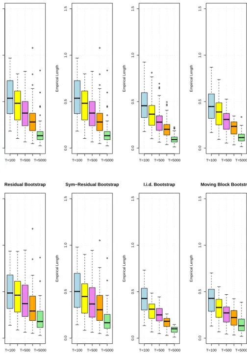
T=100 T=500 T=5000 0.0 0.5 1.0 1.5 Residual Bootstrap Empir ical Length T=100 T=500 T=5000 0.0 0.5 1.0 1.5 Sym−Residual Bootstrap Empir ical Length T=100 T=500 T=5000 0.0 0.5 1.0 1.5 I.i.d. Bootstrap Empir ical Length T=100 T=500 T=5000 0.0 0.5 1.0 1.5
Moving Block Bootstrap
Empir ical Length T=100 T=500 T=5000 0.0 0.5 1.0 1.5 Residual Bootstrap Empir ical Length T=100 T=500 T=5000 0.0 0.5 1.0 1.5 Sym−Residual Bootstrap Empir ical Length T=100 T=500 T=5000 0.0 0.5 1.0 1.5 I.i.d. Bootstrap Empir ical Length T=100 T=500 T=5000 0.0 0.5 1.0 1.5
Moving Block Bootstrap
Empir
ical Length
Figure G.2: Boxplots of the empirical lengths across all impulse responses and all propagation horizons (52 parameter constellations in total) of nominal 90% marginal confidence intervals for T ∈ {100,250,500,1000,5000}. The first row corresponds to et,i i.i.d.∼ N(0,1) and the second row corresponds toet,i
i.i.d.
∼ 3 5t5.
H
Bootstrap
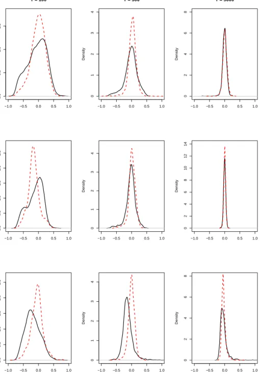
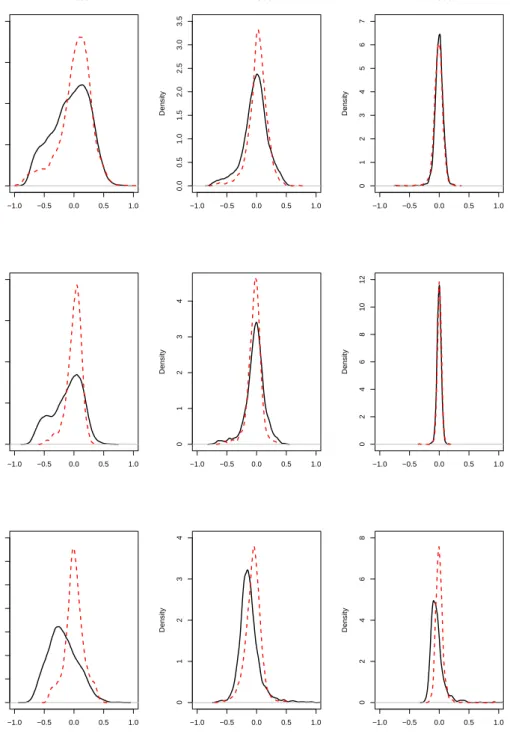
−1.0 −0.5 0.0 0.5 1.0 0.0 0.5 1.0 1.5 T = 100 Density −1.0 −0.5 0.0 0.5 1.0 0 1 2 3 4 T = 500 Density −1.0 −0.5 0.0 0.5 1.0 0 2 4 6 8 T = 5000 Density −1.0 −0.5 0.0 0.5 1.0 0.0 0.5 1.0 1.5 2.0 2.5 Density −1.0 −0.5 0.0 0.5 1.0 0 1 2 3 4 Density −1.0 −0.5 0.0 0.5 1.0 0 2 4 6 8 10 12 14 Density −1.0 −0.5 0.0 0.5 1.0 0.0 0.5 1.0 1.5 2.0 2.5 Density −1.0 −0.5 0.0 0.5 1.0 0 1 2 3 4 Density −1.0 −0.5 0.0 0.5 1.0 0 2 4 6 8 DensityFigure H.1: The simulated density of the sampling distributionΘb11,3−Θ11,3 (solid line) versus
the simulated density of the bootstrap sampling distributionΘb∗11,3−Θb11,3 (dashed line) using
the residual bootstrap. Both densities are estimated with the Epanechnikov kernel and based on 2’000 simulated observations. The first column corresponds to DGP-1a, the second column to DGP-1band the third column to DGP-1c.
−1.0 −0.5 0.0 0.5 1.0 0.0 0.5 1.0 1.5 2.0 T = 100 Density −1.0 −0.5 0.0 0.5 1.0 0.0 0.5 1.0 1.5 2.0 2.5 3.0 3.5 T = 500 Density −1.0 −0.5 0.0 0.5 1.0 0 1 2 3 4 5 6 7 T = 5000 Density −1.0 −0.5 0.0 0.5 1.0 0 1 2 3 4 Density −1.0 −0.5 0.0 0.5 1.0 0 1 2 3 4 Density −1.0 −0.5 0.0 0.5 1.0 0 2 4 6 8 10 12 Density −1.0 −0.5 0.0 0.5 1.0 0.0 0.5 1.0 1.5 2.0 2.5 3.0 3.5 Density −1.0 −0.5 0.0 0.5 1.0 0 1 2 3 4 Density −1.0 −0.5 0.0 0.5 1.0 0 2 4 6 8 Density
Figure H.2: The simulated density of the sampling distributionΘb11,3−Θ11,3 (solid line) versus
the simulated density of the bootstrap sampling distributionΘb∗11,3−Θb11,3 (dashed line) using
the symmetrized residual bootstrap. Both densities are estimated with the Epanechnikov kernel and based on 2’000 simulated observations. The first column corresponds to DGP-1a, the second column to DGP-1band the third column to DGP-1c.
−1.0 −0.5 0.0 0.5 1.0 0.0 0.5 1.0 1.5 2.0 T = 100 Density −1.0 −0.5 0.0 0.5 1.0 0 1 2 3 4 T = 500 Density −1.0 −0.5 0.0 0.5 1.0 0 1 2 3 4 5 6 7 T = 5000 Density −1.0 −0.5 0.0 0.5 1.0 0.0 0.5 1.0 1.5 2.0 Density −1.0 −0.5 0.0 0.5 1.0 0 1 2 3 Density −1.0 −0.5 0.0 0.5 1.0 0 2 4 6 8 10 12 Density −1.0 −0.5 0.0 0.5 1.0 0.0 0.5 1.0 1.5 Density −1.0 −0.5 0.0 0.5 1.0 0.0 0.5 1.0 1.5 2.0 2.5 3.0 Density −1.0 −0.5 0.0 0.5 1.0 0 2 4 6 8 Density
Figure H.3: The simulated density of the sampling distributionΘb11,3−Θ11,3 (solid line) versus
the simulated density of the bootstrap sampling distributionΘb∗11,3−Θb11,3 (dashed line) using
the i.i.d. bootstrap. Both densities are estimated with the Epanechnikov kernel and based on 2’000 simulated observations. The first column corresponds to DGP-1a, the second column to DGP-1band the third column to DGP-1c.
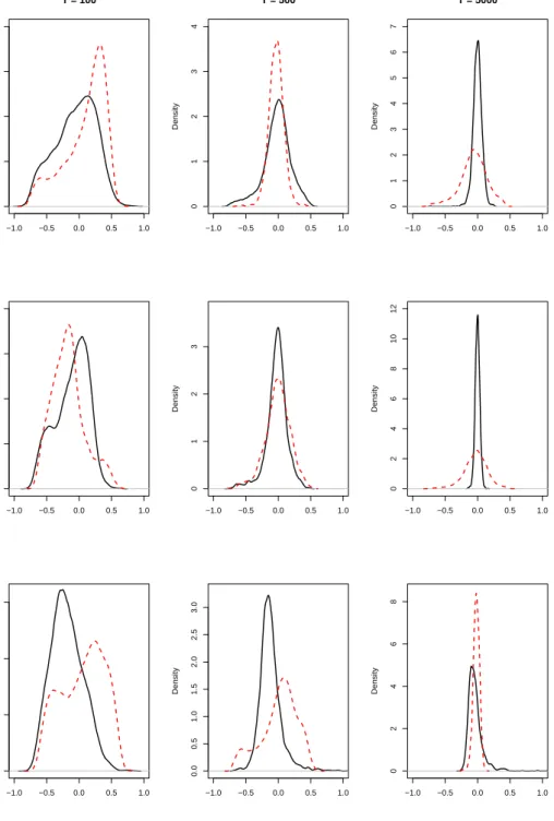
−1.0 −0.5 0.0 0.5 1.0 0.0 0.5 1.0 1.5 T = 100 Density −1.0 −0.5 0.0 0.5 1.0 0 1 2 3 4 T = 500 Density −1.0 −0.5 0.0 0.5 1.0 0 1 2 3 4 5 6 7 T = 5000 Density −1.0 −0.5 0.0 0.5 1.0 0 1 2 3 4 Density −1.0 −0.5 0.0 0.5 1.0 0 1 2 3 4 Density −1.0 −0.5 0.0 0.5 1.0 0 5 10 15 Density −1.0 −0.5 0.0 0.5 1.0 0 1 2 3 4 5 6 Density −1.0 −0.5 0.0 0.5 1.0 0 1 2 3 4 5 6 7 Density −1.0 −0.5 0.0 0.5 1.0 0 2 4 6 8 10 Density
Figure H.4: The simulated density of the sampling distributionΘb11,3−Θ11,3 (solid line) versus
the simulated density of the bootstrap sampling distributionΘb∗11,3−Θb11,3 (dashed line) using
the moving block bootstrap. Both densities are estimated with the Epanechnikov kernel and based on 2’000 simulated observations. The first column corresponds to DGP-1a, the second column to DGP-1b and the third column to DGP-1c.