Open population maximum likelihood spatial capture-recapture
This paper is currently (27 September 2017) under peer-review at a journal. Please check with the authors for a later version before citingR. Glennie
1,*, D.L. Borchers
1, M. Murchie
1, B. J. Harmsen
2,3, and R. J. Foster
2,3 1University of St Andrews, Centre for Research into Ecological and Environmental Modelling, Buchanan Gardens, St Andrews, Fife, UK
2Environmental Research Institute, University of Belize, Belmopan, Belize 3Panthera, 8 West 40th Street, 18th Floor, New York, NY, United States of America
*corresponding author:[email protected]
Abstract
Open population capture-recapture models are widely used to estimate population demographics and abun-dance over time. Bayesian methods exist to incorporate open population modelling with spatial capture-recapture, allowing for estimation of the effective area sampled and population density. Here, open population spatial capture-recapture, both Cormack-Seber and Jolly-Seber models, is formulated as a hidden Markov model, allowing inference by maximum likelihood. The method is applied to a twelve-year survey of male jaguars (Panthera onca) in the Cockscomb Wildlife Sanctuary Basin, Belize, to estimate the apparent survival and population abun-dance over time. The hidden Markov model approach is compared with Bayesian data augmentation, demonstrat-ing it to be substantially more efficient. A simulation study shows maximum likelihood inference to be negligibly bi-ased for small sample sizes and recapture rates.
1
Introduction
Many capture-recapture surveys (Seber, 1965) are con-ducted over time periods where the surveyed population undergoes change: individuals are born, immigrate, em-igrate, or die. For these methods, each individual must have a unique mark that allows detectors to record encoun-ters with them, creating their capture history. Two widely used statistical models for open populations, the Cormack-Jolly-Seber (CJS) (Cormack, 1964) and Jolly-Seber (JS) (Jolly,1965) models, use these capture histories. For CJS models, inference is restricted to those individuals whose capture histories were recorded: marked individuals. From this, the apparent survival and detectability of marked in-dividuals can be estimated. Only apparent survival is es-timable since animals that die and those that permanently emigrate are indistiguishable from their capture histories. JS models, by assuming marked and unmarked individu-als are exchangeable, extend inference to the entire pop-ulation: estimating population size over time, recruitment (birth and immigration) rate, and survival rate.
Neither CJS nor JS incorporate the spatial component in-herent in capture-recapture: individuals that range closer to a detector are more likely to be captured by that de-tector. Spatial capture-recapture (SCR) methods (Efford,
2004;Borchers and Efford,2008) do use detector locations to estimate detection probability over space. This provides a rigorous estimate of the effective area sampled and pop-ulation density.
SCR provides an efficient and flexible framework for closed population capture-recapture inference. Each individual is associated with a location in space, its activity centre. The farther an activity centre is from a detector, the less likely it is that the individual is captured by that detector. This activity centre is a latent variable: it is unobserved. Max-imum likelihood SCR modelling is achieved by numeri-cal integration, averaging over all possible activity cen-tres in the survey region. Bayesian SCR models (Royle et al.,2013b) obtain inference by sampling activity centres within a Markov chain Monte Carlo (MCMC) algorithm, using the full joint likelihood of detection parameters and activity centres. Alternatively, Bayesian inference can be obtained from the marginal likelihood where integration over activity centres is achieved by quadrature.
Existing open population SCR models (Gardner et al., 2010; Royle et al., 2013b), which are extensions of CJS and JS, rely on a Bayesian approach and the full joint likelihood of detection parameters, activity centres and life histories. Each individual has a latent life history that is sampled within an MCMC algorithm. For JS, data aug-mentation is used: a meta-population, of pre-determined size, is sampled where some individuals are born, and so contribute to the estimated population size, and some are never born. The meta-population is chosen to ensure it exceeds the size of the true population and the MCMC sampling is used to infer the distribution of the popula-tion size. This method is computapopula-tionally demanding and, when data augmentation is used, ties the interpretation of recruitment parameters to the size of the meta-population, which is determined by the analyst. No methods exist to fit open population SCR models by maximum likelihood; in particular, no algorithm other than MCMC has been used to average over all possible life histories.
In this paper, open population SCR is formulated as a hidden Markov model (HMM) (Zucchini et al.,2016), al-lowing for inference to be drawn by maximum likelihood and marginalisation over all life histories to be done ex-actly. A HMM can be described by two processes: a hidden process and a observation process. The hidden process is a Markov chain of discrete states; the observations comprise
a time series that depends on this hidden process: at each time, an observation depends only on the current state of the hidden process, and conditional on these hidden states, observations are independent. For open population SCR, the hidden process is the life history of the individual and the observations are the capture records. HMM method-ology provides an efficient algorithm to average over all possible life histories. Combined with the extant numeri-cal integration over activity centres, this allows both SCR CJS and JS models to be fit by maximum likelihood. Also, it allows for a semi-complete data likelihood to be com-puted and Bayesian inference obtained more efficiently. The JS method is applied to a camera trap survey of male jaguars (Panthera onca) in the Cockscomb Basin Wildlife Sanctuary, Belize (Harmsen et al., 2017). The survey was repeated for twelve years, between 2002 and 2015, during dry season months, between January and July. A key ques-tion for this populaques-tion is how populaques-tion size changes over time and what demographic processes drive this change. The method presented provides SCR estimates of popu-lation density, identifies which demographic rates are re-sponsible for population change, and provides a means of testing whether these rates vary over time.
Finally, a simulation study is conducted to investigate the effect of small sample size, due to low population density or low detectability, on maximum likelihood estimates. The simulation is based on the jaguar survey and estimates the bias and confidence interval coverage for each estimated parameter.
2
Methods
Consider a capture-recapture survey withKoccasions and
J detectors. During the survey,nindividuals are detected and uniquely marked, or identified to have some natural unique mark. Unique marks are used to recognise whether an individual was detected on each occasion or not: the capture history. Individuali has a capture history Ωi, a
J×K matrix, with kth column ωi,−,k and (j, k)th entry
ωi,j,k. The entries of the capture history depend on the
type of detector used: ωi,j,k= 0,1 is binary for detectors
that physically trap individuals or only register whether the individual was captured, or not, on each occasion (e.g. DNA hair traps); alternatively, ωi,j,k can be the number
of times an individual is encountered by the detector, if this is recorded (e.g. with cameras). The collection of all capture histories is denotedΩ.
In SCR, each individual is associated with a latent activity centre,xi, in two-dimensional space. The activity centre is
the spatial component of the model: it is the point in two-dimensional space that represents the average location of the individual over the survey time. In each occasion, the probability that an individual is detected on a particular detector is a decreasing function of the distance between this detector and the individual’s activity centre: those individuals that spend, on average, more time far away from the detector are detected less often than those that spend their time at a closer distance.
In open population capture-recapture, each individual has a life history, which is unobserved. On each occasionk, in-dividualihas one of three possible life states,si,k: unborn,
alive, or dead. Individuals who will be born in an occasion after occasionkand those who will immigrate into the sur-vey region after occasion kare said to be in the ‘unborn’ state; individuals that are alive in occasionkand present in the survey region are in the ‘alive’ state; finally, those individuals that died in some occasion before occasionkor emigrated from the survey region in some occasion before occasionk are said to be in the ‘dead’ state.
Here, the aim is to incorporate both SCR and open popu-lation capture-recapture into a single, tractable likelihood.
2.1
Detection model
In a particular occasion, the probability that an individ-ual is detected, and the number of times the individindivid-ual is detected by each detector, depends on the individual’s activity centre and life state. This can be described by an encounter rate model whereλj,k(xi, si,k) is the mean
num-ber of captures of individuali, with activity centre xi, on
occasion kat detectorj. Clearly, individuals that are yet to be born (or to immigrate) and those who have already died (or emigrated) cannot be detected:λj,k(xi, s) = 0 for
s= unborn, dead. For those individuals that are alive on occasion k, λj,k(xi,alive), can be specified, for example,
as a half-normal (or many other possible functional forms can be used, seeEfford(2012)).
The number of times an individual is detected in occasion
k by detector j is assumed to have a Poisson distribu-tion with mean λj,k(xi, si,k). Thus the probability that
an individual is seen at all in occasion k by detector j,
pj,k(xi, si,k), is
pj,k(xi, si,k) = 1−exp (−λj,k(xi, si,k))
It is equally possible to specify a form forpj,k, for example
half-normal, and deriveλj,k from this.
Given the mean encounter rate, the probability of the ob-served capture record on each occasion can be stated. If capture records are binary, only a record of whether the animal was seen or not seen in each occasion is made, then the probability is
[ωi,j,k|xi, si,k] =p ωi,j,k
i,j,k (1−pi,j,k)
1−ωi,j,k
wherepi,j,k=pj,k(xi, si,k), for brevity.
If capture records are counts, which are all assumed to be independently Poisson distributed, then
[ωi,j,k|xi, si,k] =
λωi,j,k
i,j,k exp(−λi,j,k)
ωi,j,k!
whereλi,j,k=λj,k(xi, si,k), for brevity.
The probability of the entire capture record on occasion
k, assuming detectors and detections are independent, is thus [ωi,·,k|xi, si,k] = J Y j=1 [ωi,j,k|xi, si,k]
If detections are not independent, then detectors are com-peting and [ωi,−,k|xi, si,k] has a multinomial distribution.
This can occur, for example, when physical trapping of the individual in one detector removes the possibility of being captured in another detector for that occasion.
2.2
Open population model
Two popular models in open population capture-recapture are the Cormack-Jolly-Seber (CJS) and the Jolly-Seber (JS) model. For CJS, individuals are known to be alive from the first occasion they are studied: individuals can only have life states that are ‘alive’ or ‘dead’. The proba-bility that an individual alive in the study region in occa-sionk survives until occasion k+ 1 is called the survival probability on occasionk and is denotedφk. In
particu-lar, only the capture histories of those individuals that are marked, captured at least once, are used and so the popu-lation studied, the popupopu-lation of marked individuals, has known size.
For JS, individuals can be born, as well as survive and die, during a survey. Furthermore, JS models assume un-marked individuals are exchangeable with un-marked indi-viduals, that is, their capture history arises from the same model. This assumption allows JS models to estimate the number of individuals ever to have lived during the survey,
N. In SCR, the total number of individuals with activity centre xis often assumed to be Poisson distributed with rateD(x). This rate is interpreted as the density at loca-tionx. When incorporated with the JS model, this inter-pretation changes. Each individual is assigned an activity centre, just as before, at location x with rateD(x), but that individual is, possibly, only alive for some number of occasions.
Conceptually, all individuals are placed in a queue: some wait to enter the queue (‘unborn’), some are in the queue (‘alive’), and some have left the queue (‘dead’). The esti-mate ˆN is the estimated number who were in the queue at some point. TheN individuals are divided among the
koccasions: some are in the queue from occasion 1, some join in occasion 2, and so on. The probability that an in-dividual is selected to join the queue in occasionkis αk.
For example,α1is the probability that an individual is in
the queue at the beginning of the survey, that is, is alive from the beginning;α2 is the probability that an
individ-ual is born or immigrates in occasion 2. Equivalently, the probability that an individual enters the queue on occa-sionk given it has not entered up to that time is denoted
βk where βk = ( α1 :k= 1 αk Qk−1 l=1(1−βl) :k >1
Similarly, individuals leave the queue in occasion k with probability 1−φk.
This queue can be described by a Markov chain. The life state of an individual in an occasion depends only on its state in the previous occasion, satisfying the Markov prop-erty. A Markov chain is fully specified by its initial distri-bution and transition probability matrix.
For CJS, the initial distributionδis known, all individuals begin in the alive state:
δ=
alive dead
( 1 0 )
For JS, the initial distribution depends on an estimable parameter:
δ=
unborn alive dead (1−α1 α1 0 )
The transition probability matrix for CJS is
Γk= alive dead φk 1−φk alive 0 1 dead For JS, Γk=
unborn alive dead !
1−βk βk 0 unborn
0 φk 1−φk alive
0 0 1 dead
Note that βk and not αk is used as it is the conditional
probability of being born, given the individual hasn’t been born up to that time, that is needed. This implicitly uses the knowledge that an individual in the ‘unborn’ state must have been in this state for all past occasions.
2.3
Hidden Markov Model
Hidden Markov models are applied to time series data where observed records at each time point depend on an unobserved Markov chain. Here, the capture history of an individual is recorded over time, and each capture record depends on the unobserved life state of that individual, where life states follow a Markov chain. Therefore, CJS and JS are examples of hidden Markov models.
Incorporating SCR with this formulation is simple. Con-ceptually, for each occasion, individuals in the queue (those that are alive) are either recorded or not depending on their activity centre. Following hidden Markov model methodology, this is described by a matrix, termed here the detection matrix.
For CJS, the detection matrix for occasionkis
Pk(xi) =
alive dead
[ωi,−,k|xi, si,k= alive] 0
0 [ωi,−,k|xi, si,k = dead]
The detection matrix for JS is similar: a 3×3 diagonal matrix with diagonal entries [ωi,−,k|xi, si,k = s] for s =
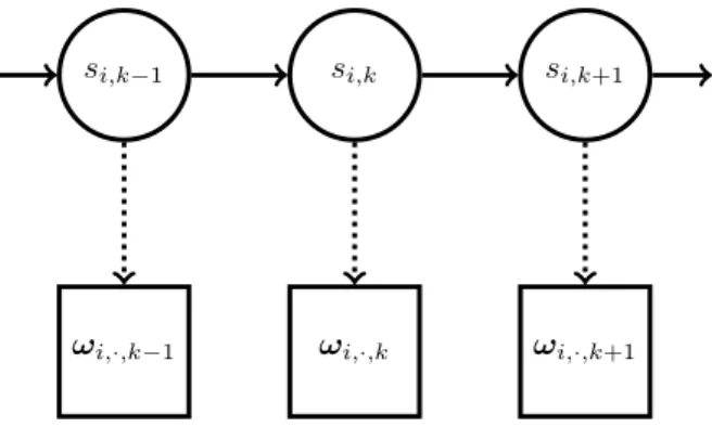
si,k−1 si,k si,k+1
ωi,·,k−1 ωi,·,k ωi,·,k+1
Figure 1. HMM formulation of open population spatial capture-recapture model: individualihas life statesi,k and
capture record (over all detectors)ωi,·,k in occasionk. Life
history is a hidden Markov process and capture records are independent conditional on life history. Nodes represent random variables and arrows terminate on variables whose distribution is defined conditional on the variable from whence the arrow originated. Unconnected nodes are conditionally independent given their parent nodes.
The power of recognising this to be a hidden Markov model is clear when it comes to averaging over all possible life histories, weighting each by their probability. It is simply a matrix product:
[Ωi|xi] =δPi,1Γ1Pi,2Γ2. . .Γi,K−1Pi,K
where Pi,K = PK(xi) and is a column vector of ones
with the appropriate size.
2.4
Spatial model
Until now, the activity centre of each individual has been treated as known. The conditional probability [Ωi|xi]
must be averaged over all possible activity centres to com-pute the unconditional likelihood of each capture history, [Ωi]. Here, it is assumed that activity centres are
dis-tributed according to a, possibly inhomogeneous, Poisson process with intensityD(x) at spatial location x.
For CJS, the number of individuals,n, is fixed and known; thus, the distribution of these activity centres are realised from a binomial point process:
[x1,· · ·,xn] = 1 n! n Y i=1 D(xi) ¯ D
where ¯D=RD(x) dx, the total intensity of activity cen-tres over all space.
For JS, the number of observed individuals,n, is a random quantity that depends on the probability of an individual being seen at least once. The set of all activity centres, for the whole population, is thinned to create a subset of those individuals that were seen. Clearly, individuals with activity centres closer to the detectors are more likely to be included in this subset. The probability of an animal with activity centre at x being seen at least once, p(x), is the thinning probability. The resultant set of activity
centres arises from a thinned Poisson process with rate
D(x)p(x) at locationx. The thinning probability is com-puted easily: the probability of being seen at least once is the complement of the probability of never being seen: if Ω0is the capture history of an individual that is never seen
by any detector on any occasion, thenp(x) = 1−[Ω0|x]
is the probability of being seen at least once during the survey with activity centre x. The probability density of the activity centres is then given
[x1,· · ·,xn] = 1 n! n Y i=1 D(xi)p(xi) exp(−D(xi)p(xi))
2.5
Likelihood
The likelihoodL, assuming individuals to be independent, is now tractable.
For CJS, the likelihood is L= [Ω] = Z [x1, . . . ,xn] n Y i=1 [Ωi|xi] dx1· · ·xn
For JS, asnis a random quantity, only the capture histo-ries of those animals seen at least once are observed, thus the likelihood is L= [Ω] =p−· n Z [x1, . . . ,xn] n Y i=1 [Ωi|xi] dx1· · ·xn
where p· =Rp(x)[x] dxis the probability of being seen at least once averaged over activity centrex.
The integration of all possible activity centres is performed by simple quadrature.
Maximum likelihood estimation can be used to obtain point, variance and interval estimates of all parameters in the standard way; similarly, priors can be specified for parameters and MCMC used with this semi-complete data likelihood.
2.6
Abundance
For JS models, the total number of individuals to have lived at some time during the survey is estimated:
ˆ
N =
Z ˆ
D(x) dx
This quantity, however, is rarely of interest. The true in-terest lies in estimating abundance over time. The mean estimated density in occasionkcan be computed:
ˆ
Dk(x) =D(x)δΓ1. . .Γk−11
where1 is the 3×1 vector (0,1,0). The estimated
abun-dance is then derived in the usual way: ˆNk=RDˆk(x) dx.
When parameters are estimated by maximum likelihood, the variance and confidence intervals for ˆNk can be
ob-tained by parametric bootstrap, sampling from the asymp-totic distributions of the maximum likelihood estimators. If Bayesian estimation were used, posterior inference for
Nk is obtained trivially from the above formula and the
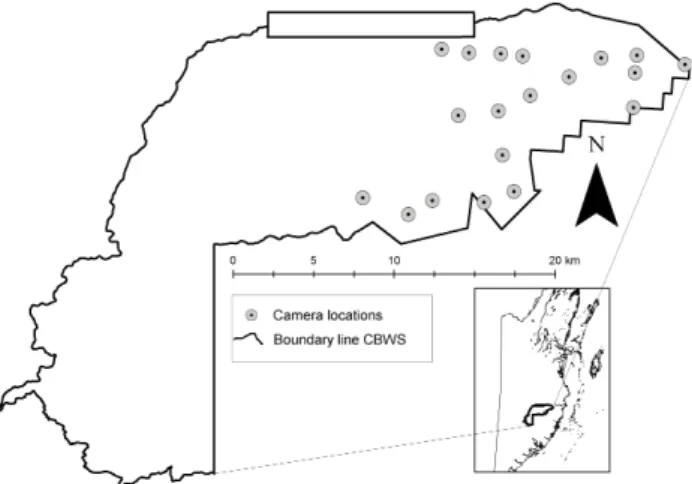
Figure 2. Cockscomb Basin Wildlife Sanctuary, Belize with approximate positions of camera traps during the survey.
3
Application: Jaguars
The aim is to estimate the population size and demo-graphics over time of male jaguars in the Cockscomb Basin Wildlife Sanctuary, Belize (Harmsen et al., 2010). Capture-recapture camera trap surveys were conducted for each year between 2002−2008 and 2011−2015. Each survey was considered an occasion and capture histories comprised counts of the number of times each jaguar was seen on each camera trap. A total of 21 camera traps were used at some time during the survey. Nineteen of the cam-eras remained in the same position for each survey. Over 12 occasions, 53 unique male jaguars were detected with an average of 23.4 detections per individual.
3.1
Model
A SCR Jolly-Seber model was fit to the data with param-eters:λ0 (mean encounter rate at a camera), σdetection
range of a camera,φapparent survival rate,β arrival rate (birth/immigration), and density D. Density necessarily changes with time; models were considered where each pa-rameter could be constant across occasions or a separate value be estimated for each occasion. The models were compared by AIC (Table1).
λ0 σ φ β ∆AIC M1 3 3 – 3 0 M2 3 3 3 – 2.5 M3 – 3 3 – 5.7 M4 – 3 3 3 12 M5 – 3 – 3 15.5
Table 1.Models (M1 – M5) with the five lowest AIC among all models;∆AIC is the difference between each model’s AIC and the lowest AIC attained among all models. Each model has parametersλ0 (mean encounter rate at a detector),σ (detection range),φ (survivial probability), andβ(arrival rate) that are constant across occasions (–) or time-varying (3).
The model with lowest AIC had constant survival proba-bility ˆφ= 0.85. Encounter rateλ0, detection rangeσ, and
arrival rateβvaried by occasion. Mean detection probabil-ity per occasion was 0.42. Detectability increased sharply from 0.39 before 2011 to 0.44 after 2011. This is presumed to be due to the cameras being changed from film to dig-ital: the model has identified this effect. Estimated mean density was estimated for each occasion (Figure3) with an average density of 1.73 per 100 square kilometres. There was no statistical evidence that density changed over time (Figure 4). These conclusions are similar to those drawn byHarmsen et al.(2017) on the same population. The number of arrivals appears constant across most years (Figure 5) except between occasions 2007 − 2008 and 2008−2010 where less arrivals, births/immigrations, oc-curred. The average density of arrivals is 0.38 per 100 square kilometres. By contrast, the estimated arrival den-sity in 2007−2008 is 0.17 per 100 square kilometres. The estimated arrival density between 2008−2010 is 0.56; this, however, spans a longer time period, 3 years, and so the average annual arrival rate is 0.19 per 100 square kilome-tres.
3.2
Comparison with augmentation
For comparison, the simplest model, that with no time-varying parameters, was fit using the augmentation ap-proach (proposed inGardner et al.(2010)) and the max-imum likelihood method presented here. The Bayesian method was implemented inrjags 4.6(Plummer,2013) with weakly informative priors.
Both methods were implemented on a desktop Intel(R) Core(TM) i7-4790 CPU (@3.6 GHz) with a cache size of 8 Gb and 16 Gb of RAM. Furthermore, both models were fit using four processor cores under similar working condi-tions. Maximum likelihood inference was obtained in 5.5 minutes, while inference by data augmentation took 23 hours to obtain a sample from the posterior, requiring around 100000 iterations. Inference from the two meth-ods was similar, differing most in the estimated detection range,σ(Table2). This discrepancy may be due to the low effective sample size achieved (<1000) for the parameter
σ.
MLE Bayes MLE CI Bayes CI
λ0 0.05 0.05 (0.04, 0.05) (0.04, 0.06) σ 5163 5546 (4892, 5448) (5061, 6494) α1 0.22 0.23 (0.12, 0.36) (0.1, 0.48) φ 0.82 0.81 (0.76, 0.87) (0.74, 0.87) ¯ N 21 20 (16, 24) (15, 24) Table 2. Maximum likelihood point estimates (MLE) and 95%confidence intervals (MLE CI) compared with data augmentation approach with Bayesian posterior means(Bayes) and95%credible intervals (Bayes CI) for mean encounter rateλ0, detection range σ, probability of being alive in the first occasionα1, survival probabilityφand average number of jaguars alive in each occasionN¯.
● ● ● ● ● ● ● ● ● ● ● ● 0.5 1 1.5 2 2.5 3 2002 2003 2004 2005 2006 2007 2008 2009 2010 2011 2012 2013 2014 2015
Year
Density per 100 square kilometres
Figure 3. Estimated density per 100 square kilometres (solid line) of male jaguars in the Cockscomb Basin Wildlife Sanctuary, Belize for each occasion (points) with lower(dashed line) and upper (dotted line)95%approximate confidence interval bounds estimated by parametric bootstrap with1000resamples.
● ● ● ● ● ● ● ● ● ● ● −0.5 0 0.5 1 2003 2004 2005 2006 2007 2008 2009 2010 2011 2012 2013 2014 2015
Year
Rate of change in density per 100 square kilometres
Figure 4.Estimated change in density per 100 square kilometres (solid line) of male jaguars in Cockscomb Wildlife Sanctuary, Belize (points) with lower(dashed line) and upper (dotted line)95%approximate confidence interval bounds estimated by parametric bootstrap with1000resamples. Horizontal line at zero density change (dot-dash line) given for reference.
● ● ● ● ● ● ● ● ● ● ● 0 0.2 0.4 0.6 0.8 1 1.2 1.4 2003 2004 2005 2006 2007 2008 2009 2010 2011 2012 2013 2014 2015
Occasion
Density of arr
iv
als per 100 square kilometres
Figure 5. Estimated annual density of arrivals per 100 square kilometres (solid line) of male jaguars in Cockscomb Wildlife Sanctuary, Belize from each survey year (points) with lower(dashed line) and upper (dotted line)95% approximate confidence interval bounds estimated by parametric bootstrap with1000resamples.
data augmentation was 250 times faster, provided simi-lar inference, and avoided auto-correlation issues common when MCMC is applied to models with latent temporal processes.
4
Simulation study
The bias in maximum likelihood estimation of density and survival was investigated by simulation. Surveys identical to the jaguar survey, with the same camera locations and number of occasions, were simulated. The survival proba-bilityφ, detection rangeσand arrival ratesα, we set equal to the estimates given in Table2. For each of six scenar-ios, 100 surveys were simulated. The percentage bias and 95% confidence interval coverage was calculated for each parameter.
For three scenarios, the true density of activity centres
D took three values 0.5 ˆD,Dˆ, and 2 ˆD where ˆD was the density estimated from the model fit in section3.2. Mean bias in density estimation was small < 5%, even when the mean unique number of individuals sighted over the entire survey were few,n= 27 (Table3). Bias in survival probability was negligible (< 1%). Coverage for density estimation was nominal on average and only slightly less than nominal (94%) on average for survival probability. Three further scenarios considered the effect of detection probability on bias. Mean encounter rateλ0took three
val-ues 0.5 ˆλ0, ˆλ0, and 2 ˆλ0 where ˆλ0 was the estimated mean
encounter rate in 2. Bias in density estimation was simi-lar to previous scenarios and confidence interval coverage
nominal on average. Bias in survival probability was larger when the number of recaptures per individual were fewer, however, bias was negligible. Confidence interval coverage was nominal on average for survival probability.
n D bias Dcoverage φbias φcoverage
27 1.2 96.1 -0.4 95.0
55 2.7 95.2 0.0 96.0
107 1.1 94.5 -0.4 92.0
Table 3. Estimated percentage bias in density of activity centresD and survival probabilityφwith Monte Carlo error (SE) computed from100simulations of the fitted jaguar model with no time varying parameters, for each of three surveys withnunique individuals seen on average
m D bias D coverage φbias φcoverage
17 1.3 94.0 -1.3 95.0
32 2.8 95.4 -0.7 94.0
62 1.2 94.5 -0.0 98.0
Table 4. Estimated percentage bias in density of activity centresD and survival probabilityφwith Monte Carlo error (SE) computed from100simulations of the fitted jaguar model with no time varying parameters, for each of three surveys with an average ofm recaptures per individual
Overall, the simulation study indicates that inference on density and survival obtained by maximum likelihood is negligibly biased, even when populations are sparse or an-imals cryptic.
5
Discussion
Formulating open population spatial capture-recapture (SCR) as a hidden Markov model (HMM) brings several advantages. The efficient algorithm that exists to compute a HMM likelihood makes the open population SCR like-lihood, marginalised over all activity centres, tractable. Similar to the use of closed population SCR, this allows the method to produce inference in a simple, efficient way. Furthermore, it brings the potential to fit more sophisti-cated models, for example, with time-varying parameters, and perform model selection in a practical time frame. The theoretical framework presented is general, incorpo-rating Cormack-Jolly-Seber and Jolly-Seber models, al-lowing inference to be obtained by maximum likelihood or Bayesian methods. Here, maximum likelihood was imple-mented and shown to produce negligibly biased inference, even when sample size or recapture rate was low. Com-pared with an augmentation approach, maximum likeli-hood inference was similar in this case and obtained sub-stantially faster. This is not a comparison of maximum likelihood and Bayesian approaches; it is a comparison of augmentation and marginalisation. A Bayesian semi-complete data likelihood approach would also be more ef-ficient than augmentation. Sampling correlated temporal processes within a Markov chain Monte Carlo (MCMC) algorithm often leads to poor mixing and low effective sample size, requiring long chains to be generated. When interest lies in the demographic parameters and not the personal histories of each individual, numerical marginali-sation over life histories, possible using a HMM algorithm, leads to better mixing and thus faster convergence to the posterior distribution. For complex models, in particular, where parameters vary over time or detection probabil-ity is heterogeneous, improving mixing can improve the inferences obtained.
5.1
Assumptions
The assumptions made in open population SCR are the combination of those made in SCR and those made in capture-recapture open population modelling:
1. Animals have unique marks that do not change during the survey.
2. Marks are recorded correctly; animals are not misidentified.
3. Animals are independent. The life history, detection probability, and activity centre of an animal is inde-pendent of all other animals.
4. Animals are exchangeable, that is, animals with the same activity centre and life history, are equally likely to be detected and, if unborn, to be born (immigrate), or, if alive, to die (emigrate). For CJS, the animals referred to are solely those that are marked, while for JS it refers to all animals in the population.
5. Emigration from the survey region is permanent.
5.2
Extensions
The proposed method is flexible and can be extended to integrate further population structure, obtain more de-tailed inference, and incorporate auxiliary data. In par-ticular, all extensions available for closed population SCR can be adapted to this context, e.g., covariates (Borchers and Efford,2008), telemetry (Royle et al.,2013b), acous-tics (Borchers et al., 2015; Stevenson et al., 2015), non-euclidean distance metrics (Royle et al.,2013a), and mix-ture modelling (Pledger, 2000). In particular, covariates can be included to explain variability in detection, prob-ability, density and demographic rates, e.g., age and sex structured inference can be obtained. Furthermore, demo-graphic rates can vary over space and time, providing in-ference on the relationship between population dynamics and habitat.
Inference on survival, rather than apparent survival, is also possible. Dispersal of an animal’s activity centre over time is unlikely to cause bias in density or survival estimates provided the animal remains within the survey region ( Er-gon and Gardner,2014). SCR modelling accounts for this movement by associating the animal with an activity cen-tre that is the average of its movement across the entire survey time; yet, if the animal emigrates from the survey region, this movement is not accounted for, and is treated as synonymous with death. Transients, animals that tem-porarily emigrate from the survey region, provide inference on this migration process. For example, if a particular an-imal is seen often by a detector, followed by a long period of time it is never seen, and then it is seen again later, this suggests the animal temporarily emigrated. Allowing for transitions of life state from dead to alive with probability
ρaccounts for this possibility. Formal statistical tests can be performed to determine ifρ >0, that is, if the capture-recapture records evince that transience occurs in the pop-ulation. Assuming that temporary emigration and perma-nent emigration occur at the same rate implies that the estimated survival probability is the true survival prob-ability and not only apparent. Whether this assumption holds strongly depends on the study population. Account-ing for dispersal directly by allowAccount-ing an animal’s activity centre to move over time has been implemented by aug-mentation (Royle et al., 2016); a method to marginalise over all possible dispersals is a focus for future work. Finally, auxiliary data on the study population can be used to improve inference on population dynamics. Recorded births or dead recoveries of marked individuals are direct observations of that individual’s life state; HMM method-ology allows for this information to be used: marginal-isation occurs only over those life histories that conform with the direct observations made. Furthermore, similar to developments in integrated population modelling (Schaub and Abadi,2011), concurrent studies on the surveyed pop-ulation, for example, records of productivity or migration, can be used. As individuals are assumed to have unique marks, these data sets need not be assumed independent; observations made directly on a marked individual can be incorporated with that individual’s life history.
5.3
Software
An R (R Core Team,2017) package,openscrpop, is avail-able on GitHub to fit the models presented in this paper:
http://github.com/r-glennie/openpopscr
References
Borchers, D., Stevenson, B., Kidney, D., Thomas, L., and Marques, T. (2015). A unifying model for capture– recapture and distance sampling surveys of wildlife pop-ulations. Journal of the American Statistical Associa-tion, 110(509):195–204.
Borchers, D. L. and Efford, M. (2008). Spatially explicit maximum likelihood methods for capture–recapture studies. Biometrics, 64(2):377–385.
Cormack, R. (1964). Estimates of survival from the sight-ing of marked animals. Biometrika, 51(3/4):429–438. Efford, M. (2004). Density estimation in live-trapping
studies. Oikos, 106(3):598–610.
Efford, M. (2012). secr: Spatially explicit capture– recapture models. r package version 2.3. 2.
Ergon, T. and Gardner, B. (2014). Separating mortality and emigration: modelling space use, dispersal and sur-vival with robust-design spatial capture–recapture data.
Methods in Ecology and Evolution, 5(12):1327–1336. Gardner, B., Reppucci, J., Lucherini, M., and Royle, J. A.
(2010). Spatially explicit inference for open populations: estimating demographic parameters from camera-trap studies. Ecology, 91(11):3376–3383.
Harmsen, B. J., Foster, R. J., Sanchez, E., Gutierrez-Gonz´alez, C. E., Silver, S. C., Ostro, L. E., Kelly, M. J., Kay, E., and Quigley, H. (2017). Long term monitoring of jaguars in the cockscomb basin wildlife sanctuary, be-lize; implications for camera trap studies of carnivores.
PloS one, 12(6):e0179505.
Harmsen, B. J., Foster, R. J., Silver, S. C., Ostro, L. E., and Doncaster, C. P. (2010). The ecology of jaguars in the cockscomb basin wildlife sanctuary, belize. The biology and conservation of wild felids, pages 403–416. Jolly, G. M. (1965). Explicit estimates from
capture-recapture data with both death and immigration-stochastic model. Biometrika, 52(1/2):225–247. Pledger, S. (2000). Unified maximum likelihood
esti-mates for closed capture–recapture models using mix-tures. Biometrics, 56(2):434–442.
Plummer, M. (2013). rjags: Bayesian graphical models using mcmc. R package version, 3.
R Core Team (2017). R: A Language and Environment for Statistical Computing. R Foundation for Statistical Computing, Vienna, Austria.
Royle, J. A., Chandler, R. B., Gazenski, K. D., and Graves, T. A. (2013a). Spatial capture–recapture models for jointly estimating population density and landscape connectivity. Ecology, 94(2):287–294.
Royle, J. A., Chandler, R. B., Sollmann, R., and Gardner, B. (2013b). Spatial capture-recapture. Academic Press. Royle, J. A., Fuller, A. K., and Sutherland, C. (2016). Spatial capture–recapture models allowing markovian transience or dispersal. Population ecology, 58(1):53– 62.
Schaub, M. and Abadi, F. (2011). Integrated popula-tion models: a novel analysis framework for deeper in-sights into population dynamics. Journal of Ornithol-ogy, 152(1):227–237.
Seber, G. A. (1965). A note on the multiple-recapture census. Biometrika, 52(1/2):249–259.
Stevenson, B. C., Borchers, D. L., Altwegg, R., Swift, R. J., Gillespie, D. M., and Measey, G. J. (2015). A general framework for animal density estimation from acoustic detections across a fixed microphone array.
Methods in Ecology and Evolution, 6(1):38–48.
Zucchini, W., MacDonald, I. L., and Langrock, R. (2016).
Hidden Markov models for time series: an introduction using R, volume 150. CRC press.