Functional nonparametric estimation of conditional extreme quantiles

(1)

Contents lists available atScienceDirect

Journal of Multivariate Analysis

journal homepage:www.elsevier.com/locate/jmva

Functional nonparametric estimation of conditional extreme quantiles

Laurent Gardes

∗

, Stéphane Girard, Alexandre Lekina

Team Mistis, INRIA Rhône-Alpes and LJK, 655, avenue de l’Europe, Montbonnot 38334 Saint-Ismier cedex, France

a r t i c l e i n f o

Article history:

Available online 23 June 2009 AMS subject classifications: 62G32 62G05 62E20 Keywords: Conditional quantile Extreme values Nonparametric estimation Functional data

a b s t r a c t

We address the estimation of quantiles from heavy-tailed distributions when functional covariate information is available and in the case where the order of the quantile converges to one as the sample size increases. Such ‘‘extreme’’ quantiles can be located in the range of the data or near and even beyond the boundary of the sample, depending on the convergence rate of their order to one. Nonparametric estimators of these functional extreme quantiles are introduced, their asymptotic distributions are established and their finite sample behavior is investigated.

1. Introduction

An important literature is dedicated to the estimation of extreme quantiles, i.e. quantiles of order 1

−

α

with

α

tending to zero. The most popular estimator was proposed by Weissman [1], in the context of heavy-tailed distributions, and adapted to Weibull-tail distributions in [2,3]. We also refer to [4] for the general case.

In a lot of applications, some covariate information is recorded simultaneously with the quantity of interest. For instance, in climatology one may be interested in the estimation of return periods associated to extreme rainfall as a function of the geographical location. The extreme quantile thus depends on the covariate and is referred to in what follows as the conditional extreme quantile. Parametric models for conditional extremes are proposed in [5,6] whereas semi-parametric methods are considered in [7,8]. Fully nonparametric estimators have been first introduced in [9], where a local polynomial modelling of the extreme observations is used. Similarly, spline estimators are fitted in [10] through a penalized maximum likelihood method. In both cases, the authors focus on univariate covariates and on the finite sample properties of the estimators. These results are extended in [11] where local polynomial estimators are proposed for multivariate covariates and where their asymptotic properties are established.

Besides, covariates may be curves in many situations coming from applied sciences such as chemometrics (see Section5

for an illustration) or astrophysics [12]. However, the estimation of conditional extreme quantiles with functional covariates has not been addressed yet. Two statistical fields are involved in this study. On the one hand, nonparametric smoothing techniques adapted to functional data are required in order to deal with the covariate. We refer to [13–16] for overviews on this literature. We propose here to select the observations to be used in the conditional quantile estimator by a moving window approach. On the other hand, once this selection is achieved, extreme-value methods are used to estimate the conditional quantile, see [17] for a comprehensive treatment of extreme-value methodology in various frameworks.

Whereas no parametric assumption is made on the functional covariate, we assume that the conditional distribution is heavy-tailed. This semi-parametric assumption amounts to supposing that the conditional survival function decreases at a polynomial rate. To estimate the conditional quantile, we focus on three different situations. In the first one, the convergence

∗_{Corresponding author.}

E-mail address:[email protected](L. Gardes).

(2)

of

α

to zero is slow enough so that the quantile is located in the range of the data. In the second situation, the quantile is located near the boundary of the sample. Finally, in the third situation, the convergence of

α

to zero is sufficiently fast so that the quantile may be beyond the boundary of the sample. This situation is clearly the most difficult one since an extrapolation outside the range of the sample is needed to achieve the estimation.

Nonparametric estimators are defined in Section 2for each situation. Their asymptotic distributions are derived in Section3. Some examples are provided in Section4and an illustration on spectrometric data is given in Section5. Proofs are postponed to Section6.

2. Estimators of conditional extreme quantiles

LetEbe a (finite or infinite dimensional) metric space associated to a metricd. Let us denote byF

(.,

x

)

the conditional cumulative distribution function of a real random variableYgivenx

∈

Eand byq

(α,

x

)

the associated conditional quantile of order 1

−

α

defined by

F

(

q

(α,

x

),

x

)

=

1

−

α,

for allx

∈

Eand

α

∈

(

0

,

1

)

. In this paper, we focus on the case where, for allx

∈

E,F

(.,

x

)

is the cumulative distribution function of a heavy-tailed distribution. In such a situation, the conditional quantileq

(.,

x

)

satisfies, for all

λ >

0,

lim

α→0

q

(λα,

x

)

q

(α,

x

)

=

λ

−_{γ (}x)

_,

₍₁₎

where

γ (.)

is an unknown positive function of the covariatexreferred to as the conditional tail index. Loosely speaking, the conditional quantileq

(.,

x

)

decreases towards 0 at a polynomial rate driven by

γ (

x

)

. The conditional quantile is said to be regularly varying at 0 with index

−

γ (

x

)

, and this property characterizes heavy-tailed distributions. We refer to [18] for a general account on regular variation theory and to Section4.2for some examples of distributions satisfying(1).

Given a sample

(

Y1

,

x1

), . . . , (

Yn

,

xn

)

of independent observations, our aim is to build point-wise estimators of conditional

quantiles. More precisely, for a givent

∈

E, we want to estimateq

(α,

t

)

, focusing on the case where the design points

x1

, . . . ,

xnare nonrandom. To this end, for allr

>

0, let us denote byB

(

t

,

r

)

the ball centered at pointtand with radiusr

defined by

B

(

t

,

r

)

= {

x

∈

E

,

d

(

x

,

t

)

≤

r

}

and lethn,t

=

htbe a positive sequence tending to zero asngoes to infinity. The proposed estimator uses a moving window

approach since it is based on the response variablesY0

isfor which the associated covariatesx

0

isbelong to the ballB

(

t

,

ht

)

.

The proportion of such design points is thus defined by

ϕ(

h_t

)

=

1 n n

X

i=1 I

{

xi

∈

B

(

t

,

ht

)

}

and plays an important role in this study. It describes how the design points concentrate in the neighborhood oftwhenht

goes to zero, similarly to the small ball probability does, see for instance the monograph on functional data analysis [14]. Thus, the nonrandom number of observations in the sliceSt

=

(

0

,

∞

)

×

B

(

t

,

ht

)

is given bymn,t

=

mt

=

n

ϕ(

ht

)

. Let

{

Zi

(

t

),

i

=

1

, . . . ,

mt

}

be the response variablesYi0sfor which the associated covariatesx

0

isbelong to the ballB

(

t

,

ht

)

and let Z1,mt

(

t

)

≤ · · · ≤

Zmt,mt

(

t

)

be the corresponding order statistics.

In this paper, we focus on the estimation of conditional ’’extreme’’ quantile of order 1

−

α

_m_t. Here, the word ’’extreme’’ means that

α

mttends to zero asngoes to infinity, making kernel based estimators [19] non-adapted. In what follows, three situations are considered:

(S.1)

α

mt

→

0 andmt

α

mt

→ ∞

,

(S.2)

α

mt

→

0,mt

α

mt

→

c

∈ [

1

,

∞

)

and

b

mt

α

mt

c → b

c

. (S.3)

α

mt

→

0 andmt

α

mt

→

c

∈ [

0

,

1

)

,

where

b

x

c

denotes the largest integer smaller thanx. Let us highlight that, in the unconditional case, situations (S.1) and (S.3) withc

6=

0 have already been examined by Dekkers and de Haan [4], the extreme casec

=

0 being considered in [20], Theorem 5.1. A summary of their results can be found in [17], Theorems 6.4.14 and 6.4.15. In situation (S.1),

α

mtgoes to 0 slower than 1

/

mt and the point-wise estimation of the conditional extreme quantile relies on an interpolation inside the

sample, since, fromProposition 2below,q

(α

mt

,

t

)

is eventually almost surely smaller that the maximal observationZmt,mt

(

t

)

in the sliceSt. In such a situation, we propose to estimateq

(α

mt

,

t

)

by:

ˆ

q1

(α

mt

,

t

)

=

Zmt−bmtαmtc+1,mt

(

t

).

(2)

In the intermediate situation (S.2), estimator(2)can still be used, since fornlarge enough,

b

mt

α

mt

c = b

c

>

0 and thus the estimation relies on a conditional extreme value of the sample. Let us note that, ifcis not an integer, thenmt

α

mt

→

c implies

b

mt

α

mt

c → b

c

. Otherwise, ifcis an integer, then condition

b

mt

α

mt

c → b

c

is necessary to prevent the sequence

b

mt

α

mt

c

from having two adherence values andq

ˆ

1

(α

mt

,

t

)

from oscillating. In situation (S.3),

α

mt goes to 0 at the same speed or faster than 1

/

mtand the conditional extreme quantile is eventually larger thanZmt,mt

(

t

)

with positive probability e−c

≥

e−1. Thus, its estimation is more difficult since it requires an estimation outside the sample. We propose in this case

(3)

to estimateq

(α

mt

,

t

)

by:

ˆ

q2

(α

mt

,

t

)

= ˆ

q1

(β

mt

,

t

) β

mt

/α

mt

γˆn(t)

=

Zmt−bmtβmtc+1,mt

(

t

) β

mt

/α

mt

γˆn(t)

,

(3)

where

β

mt satisfies (S.1) and

γ

ˆ

n

(

t

)

is a point-wise estimator of the conditional tail index

γ (

t

)

. Such estimators have been proposed both in the finite dimensional setting [11] and in the general case [21], see also Section4.1for some examples. Note that(3)is an adaptation of Weissman estimator [1] in the case where covariate information is available. The extrapolation is achieved thanks to the multiplicative term

β

mt

/α

mt

γˆn(t)

which magnitude is driven by the estimated tail index

γ

ˆ

_n

(

t

)

. As expected, the extrapolation is all the more important as the tail is heavy.

3. Main results

We first give some notations and conditions useful to establish the asymptotic distributions of our estimators. In what follows, we fixt

∈

Eand we assume:

(A) The conditional quantile function

α

∈

(

0

,

1

)

7→

q

(α,

t

)

∈

(

0

,

+∞

)

is differentiable, the function defined by

α

∈

(

0

,

1

)

7→

∆(α,t

)

=

γ (

t

)

+

α

∂

logq

∂α

(α,

t

)

∈

(

0

,

+∞

)

is continuous and such that lim_α→0∆(α,t

)

=

0

.

Assumption (A) controls the behavior of the log-quantile function with respect to its first variable. It is a sufficient condition to obtain the heavy-tail property(1), see for instance [18], Chapter 1. For alla

∈

(

0

,

1

)

, let us introduce

¯

∆(a

,

t

)

=

sup

α∈(0,a)

|

∆(α,t

)

|

.

The largest oscillation of the log-quantile function with respect to its second variable is defined for alla

∈

(

0

,

1

/

2

)

as

ω

n

(

a

)

=

sup

logq

(α,

x

)

q

(α,

x0

)

, α

∈

(

a

,

1

−

a

), (

x

,

x0

)

∈

B

(

t

,

ht

)

2

.

Finally, letkt

∈ {

1

, . . . ,

mt

}

andJkt

= {

1

, . . . ,

kt

}

. Our first result establishes a representation in distribution of the largest

random variables of the sampleZi

(

t

)

,i

∈ {

1

, . . . ,

mt

}

.

Proposition 1. If kt

/

mt

→

0and k2t

ω

n

(

m

−₍1+_δ)

t

)

→

0for some

δ >

0, then, there exists an eventAnwithP

(

An

)

→

1as n

→ ∞

such that

logZmt−i+1,mt

,

i

∈

Jkt

|

An d

=

logq

(

Vi,mt

,

Ti

),

i

∈

Jkt

|

An

,

where V1,mt

≤ · · · ≤

Vmt,mtare the order statistics associated to the sample

{

V1

, . . . ,

Vmt

}

of independent uniform variables and

{

T1

, . . . ,

Tkt

}

are random variables in the ball B

(

t

,

ht

)

.

Note that this result is implicitly used in [21], proof of Theorem 1. We also refer to [22], Theorem 3.5.2, for the approximation of the nearest neighbors distribution using the Hellinger distance and to [23] for the study of their asymptotic distribution. Here, conditionk2

t

ω

n

(

m

−(1+δ)

t

)

→

0 shows that, the smoother the quantile function is on the sliceSt, i.e. the smaller its

oscillation is, the easier the control of the uppermost observations is, i.e the largerktcan be.

The next proposition is dedicated to the study of the position of the conditional extreme quantileq

(α,

t

)

with respect to the largest observation in the sliceSt.

Proposition 2. If

ω

n

(

m

−(1+δ)

t

)

→

0for some

δ >

0, then

•

under

(

S

.

1

)

,P

(

Zmt,mt

<

q

(α

mt

,

t

))

→

0,

•

under

(

S

.

2

)

or

(

S

.

3

)

,_P

(

Zmt,mt

<

q

(α

mt

,

t

))

→

e

−c_.

Let us first focus on situation (S.1) where the estimation of the conditional extreme quantile is addressed usingq

ˆ

1

(α

mt

,

t

)

, an uppermost order statistic chosen in the considered slice.

Theorem 1.Let

(α

mt

)

be a sequence satisfying (S.1). If

(

mt

α

mt

)

2

_ω

n

(

m

−(1+δ)

t

)

→

0for some

δ >

0then,

(

mt

α

mt

)

1/2

_ˆ

q1

(α

mt

,

t

)

q

(α

mt

,

t

)

−

1

d

→

N

(

0

, γ

2

(

t

)).

It appears that the estimator is asymptotically Gaussian, with asymptotic variance proportional to

γ

2

₍

_t

_)/(

_m

t

α

mt

)

. Thus, the heavier is the tail, the larger is

γ (

t

)

, and the larger is the variance. Besides, the asymptotic variance being inversely

(4)

proportional to

α

mt, the estimation remains more stable when the extreme quantile is far from the boundary of the sample. Considering now situation (S.2), an asymptotically Gaussian behavior cannot be expected since, in this case, the estimator is based on the

b

c

th uppermost order statistic in the considered slice.

Theorem 2. Let

(α

mt

)

be a sequence satisfying (S.2). If

ω

n

(

m

−(1+δ)

t

)

→

0for some

δ >

0then,

_ˆ

q1

(α

mt

,

t

)

q

(α

mt

,

t

)

−

1

d

→

E

(

c

, γ (

t

)),

whereE

(

c

, γ (

t

))

is a non-degenerated distribution.

The asymptotic distributionE

(

c

, γ (

t

))

could be explicitly deduced from the proof of the result. It is omitted here for the sake of simplicity. Situation (S.3) is more complex since the asymptotic distribution ofq

ˆ

2may depend both on the behavior

ofq

ˆ

1and

γ

ˆ

n. In the next theorem, two cases are investigated. In situation (i), the asymptotic distribution ofq

ˆ

2is driven by

ˆ

q1. On the contrary, in situation (ii),q

ˆ

2inherits its asymptotic distribution from

γ

ˆ

n.

Theorem 3. Let

(β

mt

)

be a sequence satisfying (S.1) and let

(α

mt

)

be a sequence eventually smaller than

(β

mt

)

. Define

ζ

mt

=

(

mt

β

mt

)

1/2_log

_(β

mt

/α

mt

)

. If

(

mt

β

mt

)

2

_ω

n

(

m −(1+δ)

t

)

→

0for some

δ >

0and there exists a positive sequence

υ

n

(

t

)

and a distributionDsuch that

υ

n

(

t

)(

γ

ˆ

n

(

t

)

−

γ (

t

))

d

→

D

,

(4)

then, two situations arise:

(i) Under the additional condition

ζ

mtmax

υ

−1 n

(

t

),

∆(β

¯

mt

,

t

)

→

0

,

(5) we have

(

mt

β

mt

)

1/2

_ˆ

q2

(α

mt

,

t

)

q

(α

mt

,

t

)

−

1

d

→

N

(

0

, γ

2

(

t

)).

(6)

(ii) Otherwise, under the additional condition

υ

n

(

t

)

max

ζ

−1 mt

,

¯

∆(βmt

,

t

)

→

0

,

(7) we have

υ

n

(

t

)

log

β

mt

/α

mt

_ˆ

q2

(α

mt

,

t

)

q

(α

mt

,

t

)

−

1

d

→

D

.

(8)

Note that, even though the main interest of this result is to tackle the case where

(α

mt

)

is a sequence satisfying (S.3), it can also be applied in the more general situation where

α

mtis eventually smaller than

β

mt. For instance, it appears that, in situation (S.2),q

ˆ

2

(α

mt

,

t

)

is a consistent estimator ofq

(α

mt

,

t

)

in the sense that the ratio converges to one in probability whereas, in view ofTheorem 2,q

ˆ

1

(α

mt

,

t

)

is not consistent. Some applications ofTheorem 3are provided in the next section. 4. Examples

In Section 4.1, the above theorem is illustrated with a particular family of conditional tail index estimators. The corresponding assumptions are simplified in Section4.2for some classical heavy-tailed distributions.

4.1. Some conditional tail index estimators

In [21], a family of conditional tail index estimators is introduced. They are based on a weighted sum of the log spacings between thektlargest order statisticsZmt−kt+1,mt

, . . . ,

Zmt,mt. The family is defined by

ˆ

γ

n

(

t

,

W

)

=

kt

X

i=1 ilog

Zmt−i+1,mt

(

t

)

Zmt−i,mt

(

t

)

W

(

i

/

kt

,

t

)

kt

X

i=1 W

(

i

/

kt

,

t

) ,

(9)

whereW

(.,

t

)

is a weight function defined on (0, 1) and integrating to one. Basing on(9)and considering

β

m,t

=

kt

/

mt, the

conditional extreme quantile estimator(3)can be written as

ˆ

q2

(α

mt

,

t

,

W

)

=

Zmt−kt+1,mt

(

t

)

k_t mt

α

mt

γˆn(t,W)

.

From [21], Theorem 2, under some conditions on the weight function,

γ

ˆ

_n

(

t

,

W

)

is asymptotically Gaussian:

(5)

Table 1

Some examples of heavy-tailed distributions. For all distributions,γ (t) >0 is the tail index andρ(t) <0 is referred to as the second-order parameter in extreme-value theory. q(α,t) ∆(α,t) Pareto α−γ (t) ₀ Fréchet α−γ (t)1 αlog 1−1α −γ (t) −γ (t) 2 α(1+O(α)) Burr α−γ (t) ₁₋_α−ρ(t)−γ (t)/ρ(t) ₋_{γ (} t)α−ρ(t)₍₁₊_O_(α−ρ(t)₎₎ whereAV

(

t

,

W

)

=

R

₀1W2

(

s

,

t

)

ds. Letting

υ

n

(

t

)

=

k 1/2 t , we obtain

ζ

mt

υ

−1 n

(

t

)

=

log

kt mt

α

mt

→ ∞

,

in situation (S.2) or (S.3), which means that condition(5)cannot be satisfied. Thus, only situation (ii) ofTheorem 3may arise leading to the following corollary.

Corollary 1. Suppose the assumptions of [21], Theorem 2 hold. Let kt

→ ∞

such that

k1_t/2∆(

¯

kt

/

mt

,

t

)

→

0 and (10)

k2_t

ω

n

(

m

−(1+δ)

t

)

→

0 for some

δ >

0

.

(11)

Let

(α

mt

)

be a sequence satisfying

(

S

.

2

)

or

(

S

.

3

)

. Then, k1_t/2 log

(

kt

/(

mt

α

mt

))

_ˆ

q2

(α

mt

,

t

,

W

)

q

(α

mt

,

t

)

−

1

d

→

N

(

0

, γ

2

(

t

)

AV

(

t

,

W

)).

As an example, one can use constant weights WH

(

s

,

t

)

=

1 to obtain the so-called conditional Hill estimator with AV

(

t

,

WH

₎

₌

_{1 or logarithmic weights}_WZ

₍

_s

_,

_t

₎

_{= −}

_log

₍

_s

₎

_{leading to the conditional Zipf estimator with}_AV

₍

_t

_,

_WZ

₎

₌

_2.

We refer to [21], Section 4, for further details.

4.2. Illustration on some heavy-tailed distributions

Standard Pareto distribution is the simplest example of heavy-tailed distribution. Its conditional quantile of order 1

−

α

decreases as a power function of

α

since, in this case,q

(α,

t

)

=

α

−γ (t)_{. Therefore}_∆(α,_t

₎

₌

_{0 for all}

_α

_∈

₍

₀

_,

₁

₎

_and

condition(10)ofCorollary 1vanishes. Another example is Fréchet distribution for which

q

(α,

t

)

=

α

−γ (t)

1

α

log

1 1

−

α

−γ (t)

.

Here, the conditional quantile approximatively decreases as a power function of

α

since, in this case,q

(α,

t

)

∼

α

−γ (t)_{, the}

quality of this approximation being controlled by ∆(α,t

)

= −

γ (

t

)

2

α(

1

+

O

(α))

as

α

→

0

.

A similar example is given by Burr distributions for which

q

(α,

t

)

=

α

−γ (t) 1

−

α

−ρ(t)

−γ (t)/ρ(t) and

∆(α,t

)

= −

γ (

t

)α

−ρ(t)

(

1

+

O

(α

−ρ(t)

)),

with

ρ(

t

) <

0. These results are collected inTable 1. In both Fréchet and Burr cases,∆(α,t

)

is asymptotically proportional to

α

−ρ(t)as

α

→

0 with the convention

ρ(

t

)

= −

1 for the Fréchet distribution. Note that

ρ(

t

)

is known as the second-order parameter in the extreme-value theory. It drives the quality of the approximation of the conditional quantileq

(α,

t

)

by the power function

α

−γ (t)_{. Furthermore, it is easily seen, that for these two distributions, the function}

_|

_∆(.,_t

₎

_|

_{is increasing.}

Thus, condition(10)ofCorollary 1can be simplified asm2_tρ(t)k_t1−2ρ(t)

→

0 which shows that, the smaller

ρ(

t

)

is, the larger

ktcan be. Finally, if

γ

and

ρ

are Lipschitzian, i.e. if there exist constantscγ

>

0 andcρ

>

0 such that

|

γ (

x

)

−

γ (

x0

)

| ≤

c_γd

(

x

,

x0

)

and

|

ρ(

x

)

−

ρ(

x0

)

| ≤

c_ρd

(

x

,

x0

)

for all

(

x

,

x0

₎

_∈

_B

₍

_t

_,

_h

t

)

2, then the oscillation can be bounded by

ω

n

(

a

)

=

O

(

htlog

(

1

/

a

))

asa

→

0 and thus condition(11)

ofCorollary 1can be simplified ask2_thtlogmt

→

0

.

5. Finite sample behavior

In this section, we propose to illustrate the behavior of our conditional extreme quantile estimators on functional spectrometric data. A question of interest for the planetologist is the following: Given a spectrum collected by the OMEGA

(6)

0.0 0.2 0.4 0.6 0.8 100 150 200 250 0 5

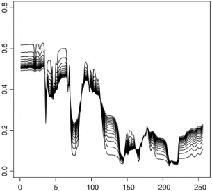
Fig. 1. Representation of the 16 spectra as functions of the wavelength.

instrument onboard the European spacecraft Mars Express in orbit around Mars, how to estimate the associated physical properties of the ground (grain size of CO2, proportions of water, dust and CO2, etc . . . )? To answer this question, a learning

dataset can be constructed using radiative transfer models. Here, we focus on the CO2proportion. Given different values yi,i

=

1

, . . . ,

16 of this proportion, a radiative transfer model provides us the corresponding spectraxi,i

=

1

, . . . ,

16

(seeFig. 1). Clearly, the obtained spectra are nonrandom. They are functions of the wavelength and we consider here their discretized version on 256 wavelengthsxi,l. Using this learning dataset, a lot of methods can be found in the literature to

estimate the CO2proportion associated to an observed spectrum. One can mention Support Vector Machine, Sliced Inverse

Regression, nearest neighbor approach, . . . (see for instance [24] for an overview of these approaches). For all these methods, the estimation of the CO2proportion is perturbed by a random error term. We propose to modelize this perturbation by:

Yi,j

=

log

(

1

/

yi

)

+

σ (

j

(

xi

)

−

Γ

(

1

−

γ (

xi

))),

j

=

1

, . . . ,

ni

,

i

=

1

, . . . ,

16

,

where

γ (

xi

)

=

0

.

3

k

xi

k

22

−

min_l

k

xl

k

22 max l

k

xl

k

22

−

min_l

k

xl

k

22

+

0

.

2

,

σ

=

min i log

(

1

/

yi

)

Γ

(

1

−

γ (

xi

))

,

and

j

(

xi

)

,j

=

1

, . . . ,

niare independent and identically distributed random values from a Fréchet distribution with tail

index

γ (

xi

)

(seeTable 1). Note that

k

xi

k

22is an approximation of the total energy of the spectrumxi. The above definitions

ensure that

γ (

xi

)

∈ [

0

.

2

,

0

.

5

]

and thatYi,j

>

0 for alli

=

1

, . . . ,

16 andj

=

1

, . . . ,

ni. Furthermore, since the expectation

of

j

(

xi

)

is given byΓ

(

1

−

γ (

xi

))

, the random variablesYi,jare centered on the value log

(

1

/

yi

)

. Our aim is to estimate the

conditional quantile

q

(α,

xi

)

= ¯

F←

(α,

xi

),

fori

=

1

, . . . ,

16

,

whereF

¯

(.,

xi

)

is the survival distribution function ofYi,1. To this end, the estimatorq

ˆ

2

(α,

xi

,

WZ

)

defined in Section4.1is

considered. The semi-metric distance based on the second derivative is adopted, as advised in [14], Chapter 9:

d2

(

xi

,

xj

)

=

Z

x(_i2)

(

t

)

−

x(_j2)

(

t

)

2 dt

,

wherex(2)denotes the second derivative ofx. To compute this semi-metric, one can use an approximation of the functions

xiandxjbased on B-splines as proposed in [14], Chapter 3. Here, we limit ourselves to a discretized versiond

˜

ofd:

˜

d2

(

xi

,

xj

)

=

255

X

l=2

(

xi,l+1

−

xj,l+1

)

+

(

xi,l−1

−

xj,l−1

)

−

2

(

xi,l

−

xj,l

)

2

.

The finite sample performance of the estimator in assessed on N

=

100 replications of the sample

{

(

xi

,

Yi,j

),

i

=

1

, . . . ,

16

,

j

=

1

, . . . ,

ni

}

withn1

= · · · =

n16

=

100. Two values of

α

are considered: 1

/

300 and 1

/

500. In the following, we

assume that the hyperparametershtandktdoes not depend on the spectrum (we thus omit the indext). These parameters

are selected thanks to the heuristics proposed in [21] which consists in minimizing the distance between two different estimators of the conditional extreme quantile:

(

_h

ˆ

select

,

k

ˆ

select

)

=

arg min

h,k ∆(

ˆ

(7)

0e+00 1e–05 2e–05 3e–05 4e–05 0 2 04 06 08 0

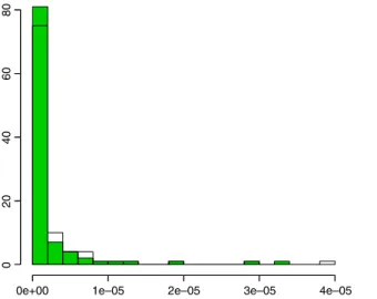
Fig. 2. Comparison between the error distributions obtained with the heuristic method (transparent) and the oracle method (gray) onN=100 samples.

0.000 0.001 0.002 0.003 0.004 0.005 15 10 0 5

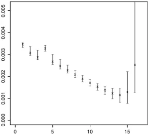
Fig. 3. 90% empirical confidence intervals ofqˆ2(1/300, .,WZ₎_{ranked by ascending order of the tail index.}

where for two functionsfandg, ∆(f

,

g

)

=

(

₁₆

X

i=1

(

f

(

xi

)

−

g

(

xi

))

2

)

1/2

.

The estimator associated to these parameters is denoted byq

ˆ

select. We also computeh

ˆ

oracleandk

ˆ

oracledefined as:

(

_h

ˆ

oracle

,

k

ˆ

oracle

)

=

arg min

h,k ∆(

ˆ

q2

(α, .,

WH

),

q

(α, .)).

The conditional quantile estimator associated to these parameters is denoted byq

ˆ

oracle. Note thath

ˆ

select,k

ˆ

select,h

ˆ

oracleand

ˆ

koracledo not depend on

α

. Of course, the oracle method cannot be applied in practical situations whereq

(α, .)

is unknown.

However, it provides us the lower bound on the distance∆that can be reached with our estimator. In order to validate our choice ofh

ˆ

selectand

ˆ

kselect, the histograms of∆(q

ˆ

select

(α, .,

WZ

),

q

(α, .))

and∆(q

ˆ

oracle

(α, .,

WZ

),

q

(α, .)),

computed for the N

=

100 replications, are superimposed onFig. 2. It appears that the mean errors are approximatively equal. Let us also remark that the heuristic errors seem to have a heavier right tail than the oracle errors. For each spectrumxithe empirical

90% confidence interval ofq

ˆ

opt

(α,

xi

,

WZ

)

is represented onFig. 3for

α

=

1

/

300 and onFig. 4for

α

=

1

/

500. The confidence

intervals are ranked by ascending order of the tail index. The larger the tail index is, the larger the confidence intervals are. This is in adequation with the result presented inCorollary 1. Finally, onFig. 5(

α

=

1

/

300) andFig. 6(

α

=

1

/

500), we draw estimators

ˆ

qselect

(α,

xi

,

WZ

)

andq

ˆ

oracle

(α,

xi

,

WZ

)

as a function of

k

xi

k

22on the replication giving rise to the median error

∆(q

ˆ

select

(α, .,

WZ

),

q

(α, .))

. It appears that the oracle estimator is only slightly better than the heuristic one. As noticed

(8)

0.000 0.001 0.002 0.003 0.004 0.005 10 15 0 5

Fig. 4. 90% empirical confidence intervals ofˆq2(1/500, .,WZ₎_{ranked by ascending order of the tail index.}

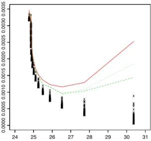
24 25 26 27 28 29 30 31 0.0000 0.0005 0.0010 0.0015 0.0020 0.0025 0.0030 0.0035

Fig. 5. Comparison of the true quantile of orderα=1/300 (solid line) with the estimated quantiles by the heuristic strategy (dashed line) and the oracle

strategy (dotted line) on the replication corresponding to the median error. The associated sample is represented by the points (‘‘×’’). 6. Proofs

6.1. Preliminary results

Our first auxiliary lemma is a simple unconditioning tool for determining the asymptotic distribution of a random variable.

Lemma 1. Let

(

Xn

)

and

(

Yn

)

be two sequences of real random variables. Suppose there exists an eventAnsuch that

(

Xn

|

An

)

d

=

(

Yn

|

An

)

withP

(

An

)

→

1. Then, Yn d

→

Y implies Xn d

→

Y .

Proof of Lemma 1. For allx

∈

_R, the well-known expansion

P

(

Xn

≤

x

)

=

P

(

{

Xn

≤

x

}|

An

)

P

(

An

)

+

P

(

{

Xn

≤

x

}|

ACn

)

P

(

A C

n

),

whereACnis the complementary event associated toAn, leads to the following inequalities: P

(

{

Xn

≤

x

}|

An

)

P

(

An

)

≤

P

(

Xn

≤

x

)

≤

P

(

{

Xn

≤

x

}|

An

)

P

(

An

)

+

P

(

ACn

).

Since

(

Xn

|

An

)

d

=

(

Yn

|

An

)

, it follows that:

(9)

24 25 26 27 28 29 30 31 0.0000 0.0005 0.0010 0.0015 0.0020 0.0025 0.0030 0.0035

Fig. 6. Comparison of the true quantile of orderα=1/500 (solid line) with the estimated quantiles by the heuristic strategy (dashed line) and the oracle

strategy (dotted line) on the replication corresponding to the median error. The associated sample is represented by the points (‘‘×’’). Taking into account of

P

(

Yn

≤

x

)

−

P

(

ACn

)

≤

P

(

{

Yn

≤

x

} ∩

An

)

≤

P

(

Yn

≤

x

)

leads to:

P

(

Yn

≤

x

)

−

P

(

ACn

)

≤

P

(

Xn

≤

x

)

≤

P

(

Yn

≤

x

)

+

P

(

ACn

).

The conclusion is then straightforward sinceP

(

Yn

≤

x

)

→

P

(

Y

≤

x

)

andP

(

ACn

)

→

0.

The next lemma provides the asymptotic distribution of extreme quantile estimators from an uniform distribution in a situation analogous to (S.1) in the unconditional case.

Lemma 2. Let V1

, . . . ,

VMbe independent uniform random variables. For any sequence

(θ

M

)

⊂

(

0

,

1

)

such that

θ

M

→

0and M

θ

M

→ ∞

,

M

θ

M

1/2

(

VbMθMc,M

−

θ

M

)

d

→

N

(

0

,

1

).

Proof of Lemma 2.For the sake of simplicity, let us introducekM

= b

M

θ

M

c

. From Rényi’s representation theorem,

VkM,M d

=

kM

X

i=1 Ei

M+1

X

i=1 Ei

whereE1

, . . . ,

EM+1are independent random variables from a standard exponential distribution. Thus,

ξ

M def

=

M

θ

M

1/2

(

VkM,M

−

θ

M

)

d

=

1 M M+1

X

i=1 Ei

!

−1

M

θ

M

1/2

×

"

1 kM kM

X

i=1 Ei

kM M

−

θ

M

+

θ

_M 1 kM kM

X

i=1 Ei

−

1

!

−

θ

_M 1 M M+1

X

i=1 Ei

−

1

!#

,

and, in view of the law of large numbers, we have

ξ

M P

∼

M

θ

M

1/2

kM M

−

θ

M

(

1

+

oP

(

1

))

+

(

M

θ

M

)

1/2 1 kM kM

X

i=1 Ei

−

1

!

−

(

M

θ

M

)

1/2 1 M M+1

X

i=1 Ei

−

1

!

def

=

ξ

₁_,_M

+

ξ

₂_,_M

−

ξ

₃_,_M

.

(10)

Let us consider the three terms separately. First, writingkM

=

M

θ

M

−

τ

Mwith

τ

M

∈ [

0

,

1

)

, we have

ξ

1,M P

∼

M

θ

M

1/2

τ

M M

=

τ

M

(

M

θ

M

)

1/2

→

0

,

(12)

sinceM

θ

M

→ ∞

. Second, sincekM

∼

M

θ

M, the central limit theorem entails

ξ

2,M

∼

k 1/2 M 1 kM kM

X

i=1 Ei

−

1

!

d

→

N

(

0

,

1

).

(13)

Similarly, it is easy to check that

ξ

3,M

=

OP

(θ

M1/2

)

=

oP

(

1

),

(14)

since

θ

M

→

0. Collecting(12)–(14)concludes the proof. 6.2. Proofs of main results

Proof of Proposition 1. Under (A) and since the random values

{

Zi

(

t

),

i

=

1

, . . . ,

mt

}

are independent, we have:

{

logZi

(

t

),

i

=

1

, . . . ,

mt

}

d

= {

logq

(

Vi

,

xi

)

i

=

1

, . . . ,

mt

}

,

wherexiis the covariate associated toZi

(

t

)

. Denoting by

ψ(

i

)

the random index of the covariate associated to the observation Zmt−i+1,mt

(

t

)

, we obtain

{

logZmt−i+1,mt

(

t

),

i

=

1

, . . . ,

mt

}

d

= {

logq

(

V_ψ(i)

,

xψ(i)

)

i

=

1

, . . . ,

mt

}

.

Let us consider the eventAn

=

A1,n

∩

A2,nwhere

A1,n

=

min i=1,...,kt−1 log q

(

Vi,mt

,

ui

)

q

(

V_i+1,mt

,

ui+1

)

>

0

,

∀

(

u1

, . . . ,

ukt

)

⊂

B

(

t

,

ht

)

and A2,n

=

min i=kt+1,...,mt logq

(

Vkt,mt

,

ukt

)

q

(

Vi,mt

,

ui

)

>

0

,

∀

(

ukt+1

, . . . ,

umt

)

⊂

B

(

t

,

ht

)

.

Conditionally toA1,n, the random variablesq

(

Vi,mt

,

ui

)

,i

=

1

, . . . ,

ktare ordered as

q

(

Vkt,mt

,

ukt

)

≤

q

(

Vkt−1,mt

,

ukt−1

)

≤ · · · ≤

q

(

V1,mt

,

u1

),

and, conditionally toA2,n, the remaining random variablesq

(

Vi,mt

,

ui

)

,i

=

kt

+

1

, . . . ,

mtare smaller since max

i=kt+1,...,mt

q

(

Vi,mt

,

ui

)

≤

q

(

Vkt,mt

,

ukt

).

Thus, conditional to An, the kt largest random values taken from the set

{

logq

(

Vψ(i)

,

xψ(i)

),

i

=

1

, . . . ,

mt

}

are

{

logq

(

Vi,mt

,

xψ(i)

),

i

=

1

, . . . ,

kt

}

. Consequently, forJkt

= {

1

, . . . ,

kt

}

and lettingTi

def

=

x_ψ(i), we have:

logZmt−i+1,mt

(

t

),

i

∈

Jkt

|

An d

=

logq

(

Vi,mt

,

Ti

),

i

∈

Jkt

|

An

.

To conclude the proof, it remains to show thatP

(

An

)

→

1 asn

→ ∞

. Let us define

δ

mt

=

m

−(1+δ)

t and consider the events A3,n

= {

V1,mt

> δ

mt

} ∩ {

Vmt,mt

<

1

−

δ

mt

}

A4,n

=

min i=1,...,kt log q

(

Vi,mt

,

t

)

q

(

Vi+1,mt

,

t

)

>

2

ω

n

(δ

mt

)

.

UnderA3,n, we have

δ

mt

<

Vi,mt

<

1

−

δ

mtfor alli

=

1

, . . . ,

mt. Hence, for all

(

ui

,

uj

)

∈

B

(

t

,

ht

)

2, it follows that, on the one

hand logq

(

Vj,mt

,

uj

)

q

(

V_i_,_m_t

,

u_i

)

=

log q

(

Vj,mt

,

t

)

q

(

V_i_,_m_t

,

t

)

+

log q

(

Vj,mt

,

uj

)

q

(

V_j_,_m_t

,

t

)

+

log q

(

Vi,mt

,

t

)

q

(

V_i_,_m_t

,

u_i

)

≥

logq

(

Vj,mt

,

t

)

q

(

Vi,mt

,

t

)

−

2

ω

n

(δ

mt

),

(11)

and on the other hand, min i=kt+1,...,mt logq

(

Vkt,mt

,

ukt

)

q

(

Vi,mt

,

ui

)

≥

min i=kt+1,...,mt logq

(

Vkt,mt

,

t

)

q

(

Vi,mt

,

t

)

−

2

ω

n

(δ

mt

)

≥

log q

(

Vkt,mt

,

t

)

q

(

Vkt+1,mt

,

t

)

−

2

ω

n

(δ

mt

).

ConsequentlyA3,n

∩

A4,n

⊂

An. Remarking that

P

(

A3,n

)

≥

P

(

V1,mt

> δ

mt

)

+

P

(

Vmt,mt

<

1

−

δ

mt

)

−

1

=

2P

(

V1,mt

> δ

mt

)

−

1

→

1

,

sinceVmt,mt

d

=

1

−

V1,mtandP

(

V1,mt

> δ

mt

)

=

1

−

δ

mt

→

1, it thus remains to prove that_P

(

A4,n

)

→

1. From [18],

paragraph 1.3.1, condition (A) implies that there existsc

(

t

) >

0, depending only ontsuch that, for all

α

∈

(

0

,

1

)

,

q

(α,

t

)

=

c

(

t

)

exp

Z

1 α

γ (

t

)

+

∆(u

,

t

)

u du

,

which is the so-called Karamata representation for normalised regularly varying functions. Hence, for alli

∈

Jkt, log q

(

Vi,mt

,

t

)

q

(

Vi+1,mt

,

t

)

=

Z

Vi+1,mt Vi,mt

γ (

t

)

+

∆(u

,

t

)

u du

,

and it follows that log q

(

Vi,mt

,

t

)

q

(

Vi+1,mt

,

t

)

≥

(γ (

t

)

− ¯

∆(Vkt+1,mt

,

t

))

log Vi+1,mt Vi,mt

,

leading to P

(

A4,n

)

≥

P

(γ (

t

)

− ¯

∆(Vkt+1,mt

,

t

))

min i=1,...,kt logVi+1,mt Vi,mt

>

2

ω

n

(δ

mt

)

≥

_P

≥

4

ω

n

(δ

mt

)

γ (

t

)

∩

_¯

∆(Vkt+1,mt

,

t

) < γ (

t

)/

2

≥

_P

≥

4

ω

n

(δ

mt

)

γ (

t

)

+

_P _∆(

¯

_V_k t+1,mt

,

t

) < γ (

t

)/

2

−

1 def

=

P1,mt

+

P2,mt

−

1

.

In view of Rényi representation for uniform ordered random variables,

{

ilog

(

V_i−_,_m1_t

/

V_i−₊1₁_,_m_t

),

i

∈

Jkt

}

d

= {

Fi

,

i

∈

Jkt

}

,

whereF1

, . . . ,

Fktare independent random variables from a standard exponential distribution, we have P1,mt

=

P

min i=1,...,kt Fi i

≥

4

ω

n

(δ

mt

)

γ (

t

)

=

kt

Y

i=1 exp

−

4i

ω

n

(δ

mt

)

γ (

t

)

=

exp

−

2

γ (

t

)

kt

(

kt

+

1

)ω

n

(δ

mt

)

→

1

,

sincek2_t

ω

n

(δ

mt

)

→

0. Furthermore,Vkt+1,mt

=

(

kt

/

mt

)(

1

+

oP

(

1

))

P

→

0 and∆(α,t

)

→

0 as

α

→

0 entailP2,mt

→

1. The conclusion follows.

Proof of Proposition 2.From Proposition 1, there exists an eventAn withP

(

An

)

→

1 such that

(

Zmt,mt

(

t

)

|

An

)

d

=

(

q

(

V1,mt

,

T1

)

|

An

)

and thus, P

(

Zmt,mt

(

t

) <

q

(α

mt

,

t

))

=

P

logq

(

V1,mt

,

T1

)

q

(α

mt

,

t

)

<

0

∩

An

+

_P

logZmt,mt

(

t

)

q

(α

mt

,

t

)

<

0

∩

AC_n

def

=

P3,mt

+

P4,mt

.

(15) Clearly,P4,mt

≤

P

(

A C

n

)

→

0. Let us now consider the termP3,mt. Introducing

δ

mt

=

m

−(1+δ) t andA5,n

= {

V1,mt

∈ [

δ

mt

,

1

−

δ

_m_t

]}

, we have P3,mt

=

P

logq

(

V1,mt

,

T1

)

q

(α

mt

,

t

)

<

0

∩

An

∩

A5,n

+

_P

logq

(

V1,mt

,

T1

)

q

(α

mt

,

t

)

<

0

∩

An

∩

AC5,n

(12)

and standard calculations lead to: P

logq

(

V1,mt

,

T1

)

q

(α

mt

,

t

)

<

0

∩

_A₅_,_n

+

_P

(

_A_n

)

−

1

≤

P3,mt

≤

P

logq

(

V1,mt

,

T1

)

q

(α

mt

,

t

)

<

0

∩

_A₅_,_n

+

_P

(

_AC₅_,_n

).

Furthermore,A5,nimplies

logq

(

V1,mt

,

T1

)

q

(

V1,mt

,

t

)

≤

ω

_n

(δ

_m_t

),

and thus P

logq

(

V1,mt

,

t

)

q

(α

mt

,

t

)

<

−

ω

_n

(δ

_m_t

)

∩

A5,n

+

_P

(

An

)

−

1

≤

P3,mt

≤

_P

logq

(

V1,mt

,

t

)

q

(α

mt

,

t

)

< ω

n

(δ

mt

)

∩

A5,n

+

_P

(

AC₅_,_n

),

which entails P

logq

(

V1,mt

,

t

)

q

(α

mt

,

t

)

<

−

ω

_n

(δ

_m_t

)

+

_P

(

A5,n

)

+

P

(

An

)

−

2

≤

P3,mt

≤

P

logq

(

V1,mt

,

t

)

q

(α

mt

,

t

)

< ω

n

(δ

mt

)

+

_P

(

AC₅_,_n

).

(16) Let us now focus on the quantity

P5,mt def

=

_P

logq

(

V1,mt

,

t

)

q

(α

mt

,

t

)

<

±

ω

_n

(δ

_m_t

)

=

P

log q

(

V1

,

t

)

q

(α

mt

,

t

)

<

±

ω

_n

(δ

_m_t

)

mt

=

_P q

(

V1

,

t

) <

e±ωn(δmt)q

(α

mt

,

t

)

mt

=

_P 1

−

V1

<

F e±ωn(δmt)q

(α

mt

,

t

),

t

mt

=

exp

mtlogF e±ωn(δmt)q

(α

mt

,

t

),

t

.

Since e±ωn(δmt)_q

(α

_m

t

,

t

)

→ ∞

and introducing the conditional survival functionF

¯

(.,

t

)

=

1

−

F

(.,

t

)

, we have mtlogF e ±_ωn(δmt)_q

(α

mt

,

t

),

t

= −

mtF

¯

e ±_ωn(δmt)_q

(α

mt

,

t

),

t

(

1

+

o

(

1

))

= −

mt

α

mt

¯

F e±ωn(δmt)_q

(α

_m t

,

t

),

t

¯

F q

(α

mt

,

t

),

t

(

1

+

o

(

1

)).

As already mentioned, (A) implies(1)which, in turn, shows thatF

¯

(.,

t

)

is a regularly function at infinity with index

−

1

/γ (

t

)

. Hence, since e±ωn(δmt)

→

1, we thus have (see [18], Theorem 1.5.2),

¯

F e±ωn(δmt)q

(α

mt

,

t

),

t

¯

F q

(α

mt

,

t

),

t

→

1

.

As a conclusion, P5,mt

=

1

−

α

_m_t

(

1

+

o

(

1

))

mt

,

(17)

and collecting(16)and(17)leads to:

1

−

α

_m_t

(

1

+

o

(

1

))

mt

+

_P

(

_A₅_,_n

)

+

_P

(

_A_n

)

−

2

≤

P3,mt

≤

1

−

α

_m_t

(

1

+

o

(

1

))

mt

+

_P

(

_AC₅_,_n

).

SinceP

(

A5,n

)

→

1 andP

(

An

)

→

1, it is then straightforward thatP3,mt

→

0 under (S.1) andP3,mt

→

e

−c_{under (S.2) or}

(S.3). Eq.(15)concludes the proof.

Proof of Theorem 1. Let us introduce, for the sake of simplicity,kt

= b

mt

α

mt

c

. FromProposition 1, there exists an event Ansuch that:

(

mt

α

mt

)

1/2_logq

ˆ

1

(α

mt

,

t

)

q

(α

mt

,

t

)

An

d

=

(

mt

α

mt

)

1/2_logq

(

Vkt,mt

,

Tkt

)

q

(α

mt

,

t

)

An

,

whereP

(

An

)

→

1. FromLemma 1, the convergence in distribution

(

mt

α

mt

)

1/2_logq

(

Vkt,mt

,

Tkt

)

q

(α

mt

,

t

)

d

(13)

is a sufficient condition to obtain

(

mt

α

mt

)

1/2_logq

ˆ

1

(α

mt

,

t

)

q

(α

mt

,

t

)

d

→

N

(

0

, γ

2

(

t

)).

A straightforward application of the

δ

-method will then conclude the proof. Let us prove the convergence in distribution(18). To this end, consider

Rn

=

logq

(

Vkt,mt

,

Tkt

)

q

(

Vkt,mt

,

t

)

and let

δ

_m_t

=

m−_t(1+δ). Remark that, under (S.1),

P

(

Rn

≤

ω

n

(δ

mt

))

≥

P

(

Vkt,mt

∈ [

δ

mt

,

1

−

δ

mt

]

)

→

1

.

Thus,R_n

=

O_P

(ω

_n

(δ

_m_t

))

and we have

logq

(

Vkt,mt

,

Tkt

)

q

(α

mt

,

t

)

=

logq

(

Vkt,mt

,

t

)

q

(α

mt

,

t

)

+

OP

(ω

n

(δ

mt

)).

(19)

Let us introduce the log-quantile functiong

(.)

=

logq

(.,

t

)

. Clearly, for all

α

∈

(

0

,

1

)

,

g0

(α)

=

∆(α,t

)

−

γ (

t

)

α

and a first-order Taylor expansion leads to:

(

mt

α

mt

)

1/2_logq

(

Vkt,mt

,

t

)

q

(α

mt

,

t

)

=

(

mt

α

mt

)

1/2_g0

_(θ

mt

)(

Vkt,mt

−

α

mt

)

=

α

_m_tg0

(θ

mt

)

mt

α

mt

1/2

(

Vkt,mt

−

α

mt

),

where

θ

mt

∈ [

min

(α

mt

,

Vkt,mt

),

max

(α

mt

,

Vkt,mt

)

]

. Now,Vkt,mt

P

∼

α

_m_tentails

θ

mt P

∼

α

_m_t

→

0 and, from (A),

α

mtg 0

_(θ

mt

)

P

∼

θ

_m_tg0

(θ

mt

)

=

∆(θmt

,

t

)

−

γ (

t

)

P

→ −

γ (

t

).

Then,Lemma 2implies that

(

mt

α

mt

)

1/2_logq

(

Vkt,mt

,

t

)

q

(α

mt

,

t

)

d

→

N

(

0

, γ (

t

)

2

).

(20)

Collecting (19) and (20) concludes the proof after remarking that condition

(

mt

α

mt

)

2

_ω

n

(δ

mt

)

→

0 implies

(

mt

α

mt

)

1/2

ω

n

(δ

mt

)

→

0.

Proof of Theorem 2. Sinceq

(.,

t

)

is regularly varying with index

−

γ (

t

)

, we have under (S.2) thatq

(

1

/

mt

,

t

)/

q

(α

mt

,

t

)

∼

(

mt

α

mt

)

γ (

t)

_→

_cγ (t)_{and the following asymptotic expansion holds}

logq

ˆ

1

(α

mt

,

t

)

q

(α

mt

,

t

)

=

logq

ˆ

1

(α

mt

,

t

)

q

(

1

/

mt

,

t

)

+

logq

(

1

/

mt

,

t

)

q

(α

mt

,

t

)

=

logq

ˆ

1

(α

mt

,

t

)

q

(

1

/

mt

,

t

)

+

γ (

t

)

log

(

c

)

+

o

(

1

).

Now, recall that in situation (S.2), fornlarge enough,

b

mt

α

mt

c = b

c

. Thus, fromProposition 1, there exists an eventAn

such that_P

(

An

)

→

1 and

logq

ˆ

1

(α

mt

,

t

)

q

(

1

/

mt

,

t

)

An

d

=

logq

(

Vbcc,mt

,

Tbcc

)

q

(

1

/

mt

,

t

)

An

.

Mimicking the proof ofTheorem 1, we obtain

logq

(

Vbcc,mt

,

Tbcc

)

q

(

1

/

mt

,

t

)

=

logq

(

Vbcc,mt

,

t

)

q

(

1

/

mt

,

t

)

+

OP

(ω

n

(δ

mt

)).

To conclude, one can remark that q

(

Vbcc,mt

,

t

)

is the

b

c

th uppermost order statistics associated to a heavy-tailed distribution. In such a case, Corollary 4.2.4 of [17] states thatq

(

Vbcc_,mt

,

t

)/

q

(

1

/

mt

,

t

)

converges to a non-degenerated