Comparison of dynamic itemset mining algorithms for multiple support thresholds

(1)

Support Thresholds

Nourhan N. Abuzayed

Department of Computer Engineering,

Izmir Institute of Technology

Izmir, Turkey

Belgin Ergenç

Department of Computer Engineering,

Izmir Institute of Technology

Izmir, Turkey

ABSTRACT

Mining1_{frequent itemsets is an important part of association rule} mining process. Handling dynamic aspect of databases and multiple support threshold requirements of items are two important challenges of frequent itemset mining algorithms. Most of the existing dynamic itemset mining algorithms are devised for single support threshold whereas multiple support threshold algorithms are static. This work focuses on dynamic update problem of frequent itemsets under multiple support thresholds and proposes tree-based Dynamic CFP-Growth++ algorithm. Proposed algorithm is compared to our previous dynamic algorithm Dynamic MIS [50] and a recent static algorithm CFP-Growth++ [2] and, findings are; in dynamic database, 1) both of the dynamic algorithms are better than the static algorithm Growth++, 2) as memory usage performance; Dynamic CFP-Growth++ performs better than Dynamic MIS, 3) as execution time performance; Dynamic MIS is better than Dynamic CFP-Growth++. In short, Dynamic CFP-Growth++ and Dynamic MIS have a trade-off relationship in terms of memory usage and execution time.

KEYWORDS

Association rule mining; itemset mining; dynamic itemset mining; multiple support thresholds

1 INTRODUCTION

Association rule mining is one of the main tasks of data mining. Lately, an intensive research focuses on it due to its applicability in many decision making processes in share market, retail sector, web log analysis, text mining, customer analysis, prediction, etc. [14]. Association rule was first introduced by Agrawal et al. [7] and is defined as, AB; meaning customers who buy item A also buy item B if the context is market basket analysis. Association rules are meant to find the impact of a set of items on another set

Permission to make digital or hard copies of all or part of this work for personal or classroom use is granted without fee provided that copies are not made or distributed for profit or commercial advantage and that copies bear this notice and the full citation on the first page. Copyrights for components of this work owned by others than ACM must be honored. Abstracting with credit is permitted. To copy otherwise, or republish, to post on servers or to redistribute to lists, requires prior specific permission and/or a fee. Request permissions from [email protected]. IDEAS '17, July 12 – 14 2017, Bristol, England

of items. An itemset (items that co-occur in a transaction) frequency is referred as the support count, which is the number of transactions that include the itemset. An itemset can be frequent if its support count satisfies the minimum support minsup threshold [27]. Confidence is another measure for association rules; confidence for an association rule XY is the ratio of transactions that include X∪Y to the count of transactions that include X [7, 9].

Association rule mining process includes two basic steps; 1) finding frequent itemsets (patterns), 2) generating association rules [8]. The first step is more expensive so it is the concentration of many studies. Various algorithms have been proposed to find the frequent patterns from huge databases. The most classical one is the Apriori algorithm [8] that uses candidate generation and testing approach to discover frequent itemsets. Other subsequent algorithms using Apriori-like technique were introduced in [15, 16, 17, 18, 19, 20, and 21]. Due to the drawback of “generate candidates and test” approach of Apriori-like algorithms, algorithms that don’t depend on candidate generation are introduced, such as FP-Growth [9] and Matrix Apriori [10 and 11].

On the other side, the essential disadvantage of these itemset mining algorithms is their dependency on single user given minsup. Single support threshold is not sufficient to represent the characteristics of the items and causes rare item problem [13]. In many applications, the occurrence of some items is frequent in the data, whereas the occurrences of the others are rare. For example, the number of breads sold in comparison to the sales of the televisions cannot be similar in a supermarket therefore we cannot distinguish them as frequent with a unique support threshold. If minsup is set too high, the rules those have rare items like television will not be discovered. In order to find rules that involve both rare and frequent items, minsup has to be set very low but this may cause combinatorial explosion of frequent items [12]. Some algorithms as MSapriori [12], Growth [1], CFP-Growth++ [2] and MISFP-Growth [29] are introduced to solve the problem of itemset mining under multiple itemset support (MIS) thresholds.

One main hypothesis in most of the above algorithms is that database is static, but in real life, databases are continuously updated. This reveals that originally discovered association rules may no longer be valid and yet new interesting rules or frequent itemsets may arise as a result of an update on the database. The most straightforward way to update the rules or frequent itemsets would be to repeat all entire mining process from the start. However this is expensive in terms of execution time and

(2)

memory, in databases like supermarket sales database with big growth rate each day. Therefore various algorithms have been introduced in [3, 4, 5, 6, 22, 23, 24, and 25]. These algorithms perform faster and use less system resources since they update frequent association rules/itemsets by considering only the updates instead of repeating all mining process from the beginning.

Most mentioned works handle either the dynamic itemset mining with single support threshold or itemset mining with multiple support thresholds (MIS), assuming that the database is static. There are few existing solutions for dynamic itemset mining under MIS [24, 26, 40 and 50]. In our previous work [50] we had proposed an algorithm (Dynamic MIS) that handles the problem of dynamic itemset mining under multiple item support thresholds in order to show the efficiency and limits of that algorithm; it was compared with a static algorithm CFP-Growth++ [2]. We had found out that Dynamic MIS requires huge memory since it keeps whole growth tree in the memory all the time. In this paper, new dynamic algorithm which is called Dynamic CFP-Growth++ is introduced. It allows dynamic itemset mining under multiple support thresholds in a style of “build once, update many and mine anytime”. It 1) uses pattern growth tree, 2) avoids candidate generation and testing, 3) handles all kinds of increments as additions, additions with new items and deletions, 4) assumes that MIS thresholds do not change during increments and 5) uses discarding property in its pre-mining phase, that allows pruning of items with the support less than minimum of MIS and provides better memory usage.

Proposed algorithm; Dynamic CFP-Growth++, is compared to our previous dynamic algorithm; Dynamic MIS [50] and static algorithm CFP-Growth++ [2] by using four databases. Execution time and memory usage performance of both dynamic algorithms over static algorithm is observed while changing the increment size. The findings are; as the time consumption 1) Dynamic MIS and Dynamic CFP-Growth++ perform better than CFP-Growth++ since they run only on increments, 2) Dynamic MIS can achieve Speed-up2_{of 56 times against CFP-Growth++, whereas the} speed-up of Dynamic CFP-Growth++ cannot exceed 2 times, 3) Dynamic CFP-Growth++ is better than CFP-Growth++ until increment size is less than 85% with large and sparse database, 25% with small and dense database. However the memory usage of Dynamic CFP-Growth++ is better than Dynamic MIS with all the datasets, this is due to its advantage provided by pruning and merging of the tree in pre-mining phase while Dynamic MIS keeps the whole tree in memory all the time.

The organization of this paper is as follows: Section 2 introduces Dynamic CFP-Growth++ algorithm with tree builder and increment handling parts. Section 3 shows the performance evaluation. Section 4 discusses the related work and Section 5 is dedicated to the conclusion remarks.

2 DYNAMIC ITEMSET MINING

In this section, a new dynamic itemset mining algorithm-Dynamic CFP-Growth++ is introduced. It maintains tree structure to keep

2_{Speed-up = Execution time}

CFP-Growth++ / Execution timeDynamic algorithm

the signatures of the transactions like FP-Growth algorithm [1]. Dynamic Growth++ is customized version of CFP-Growth++ algorithm [2] in a way to handle increments. In the first subsection, a motivating example is illustrated.

2.1 Motivating Example

Throughout the text, the following example illustrated in two tables is used. Table 1 presents a sample database D that is composed of five transactions. Table 2 illustrates the user given multiple item support (MIS) for each item in decreasing order. The last row of Table 2 presents items’ actual support in the database D. As seen from Table 2, MIN MIS (minimum of MIS) is 40%. In the right most column of Table 1, the transactions’ items are in order of support values as given in Table 2.

Table 1: Transaction database D [1]

TID Items Items (ordered)

100 D, C,A, F A, C, D, F

200 G, C, A, F, E A, C, E, F, G 300 B, A, C, F, H A, B, C, F, H

400 G, B, F B, F, G

500 B, C B, C

Table 2: MIS and actual support of items [1]

Item A B C D E F G H

MIS value (%) 80 80 80 60 60 40 40 40

Actual Support (%) 60 60 80 20 20 80 40 20

2.2 Dynamic CFP-Growth++

This algorithm builds MIS-tree as in [2] from the original database D. Each time an incremental database d arrives, it is added to the existing tree. This tree is preserved during the arrival of updates; pruning and merging operations are carried on as a preparation phase before mining.

Figure 1: MIS-tree builder.

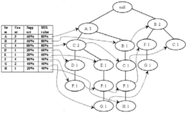
2.2.1 Building MIS-tree. Building the tree is similar to CFP-Growth++ in [2] and the result tree is shown in Figure 2 for our motivating example. Let us explain the pseudo code of MIS-tree builder algorithm with our motivating example. MISsorted list is created from the MIS values of Table 2. in decreasing order as indicated (Line 1). After that the root of MIS-tree and Min frequent item header table is created (Lines 2-3). Then the ordered items of the MISsorted are inserted into this table with item’s count 0 (Line 4). The database D is scanned, and the transactions are

INPUT: database D, Minimum support MIS

OUTPUT: MISsorted, MIS-tree

BEGIN

1 Build MISsorted list(in decreasing order)

2 Create the root of MIS-tree as null

3 Create Min frequent item header table 4 Insert items in the table (count=0)

5 Scan D

6 FOR each transaction T in D do:

7 Sort items in T (like MISsorted)

8 Add T to the tree

9 END FOR

10 Calculate the support of items in D

11 Update supports in the header table END

(3)

updated. (Lines 10-11). Fig. 2 shows the incompact tree generated with the motivating example.

Figure 2: MIS-tree for the motivating example.

2.2.2 Adding Increments. Let us explain the pseudo code of additions in Dynamic CFP-growth++ algorithm shown in Fig. 3.

Figure 3: Additions.

When new transactions arrive, they are scanned to be added to the tree. The items in the new transaction are sorted in decreasing order as MISsorted. Then transactions are added to the tree one by one. Each item’s count in this transaction is updated by incrementing its count in the primary header table by 1. Then the nodes of same item are linked all through the tree to the item in the header table of the same figure. The supports of all items in the whole database are calculated then updated in the Min frequent item header table.

2.2.3 Adding Increments with New Items. The input tree for this case is the MIS-tree of Fig. 2, incremental database and MIS values of new items. The first step is combining the new MIS values with the MIS values of the old items to get MISsorted as indicated in the Line 1 of the algorithm shown in of Fig. 4.

New items in MISnew are inserted in the Min frequent item header table with item’s count 0, this insertion is done by taking into account the MISsorted order (Line 2). Now the increment d is scanned, and then sorted according to sorted list of all items. After that; the transactions are added to the tree, then the item’s counts and node links are updated. From these counts the supports are calculated and updated in the header table.

Figure 4: Additions with new items.

2.2.4 Adding Increments with Deletions. The pseudo code of deletions in Dynamic CFP-growth++ algorithm is shown in Fig. 5. First, deletions are scanned. And then deleted from the MIS-tree, some items’ counts are decremented. From these counts supports are calculated and updated in the header tables of tree.

Figure 5: Deletions.

2.2.5 Pre-mining with Dynamic CFP-Growth++. In order to construct the compact MIS-tree; pruning and merging operations are applied as a preparation phase before mining as in the case of CFP-Growth++ algorithm [2]. The MIS-tree is constructed with every item in the transaction database. So, LMS (lowest multiple supports) and infrequent leaf node pruning, are used to reduce the search space. LMS Procedure [2] is used to prune the items that cannot generate any frequent pattern. After the tree-pruning operation ends; all the supports of the remaining items in the MIS-tree are greater than LMS value.

After LMS tree-pruning, tree-merging process (MisMerge[2]) is carried out to merge the child nodes of a parent node that share a common item. After that; the process of infrequent leaf node pruning (InfrequentLeafNodePruning Procedure [2]) is carried on the resultant MIS-tree to decrease its size. In this process, among the remaining items in the MIS-list of MIS-tree, the items that have support less than their required support are deleted only if they are leaf nodes.

Let us apply an example for the preparation of pruning and merging on the tree of Fig. 2. The MIS-tree is constructed with every item in the transaction database. So, lowest multiple support (MIN MIS) and infrequent leaf node pruning are used in pruning step to decrease the search space. MIN MIS is 2 (40%) from the MIS-tree. As a result, any item that has support less than 2 is discarded (i.e., D, H, E). The last item in the MIS-list is G that is frequent item. Hence, no tree-pruning operation is done for the

INPUT: MIS-tree, MISsorted, incremental database d

OUTPUT: Dynamic MIS-tree

BEGIN

1 Scan d

2 FOR each transaction T in d do:

3 Sort items in T (like MISsorted)

4 Add T to the tree

5 END FOR

6 Calculate the support of all items 7 Update the supports

END

OUTPUT: MISsorted, Dynamic MIS-tree

BEGIN

1 Build MISsorted (MISsorted + MISnew)

2 Insert new items into primary header table (count=0)

3 Scan d

5 Sort items in T (like MISsorted )

6 Add T to the tree

7 END FOR

8 Calculate the support of all items 9 Update the supports in the table END

INPUT: MIS-tree, MISsorted, increment d

OUTPUT: Dynamic MIS-tree

BEGIN

1 Scan d

3 Sort items in T (like MISsorted)

4 Delete T from the tree

5 END FOR

6 Calculate the support of all items 7 Update the supports in header table END

(4)

item G. The tree-pruning operation ends as the supports of the remaining items in the MIS-tree are greater than MIN MIS = 2.

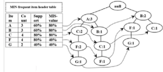
Tree-merging process is carried out to merge the child nodes of a parent node that share a common item like FP-growth given in [1] after tree pruning. The result MIS-tree is called compact MIS-tree as given in Fig. 6. The process of infrequent leaf node pruning is carried on the compact MIS-tree to decrease its size. The process is as follows, among the remaining items in the MIS-list of MIS-tree, A and B are infrequent items (i.e., their support is less than the required minsup value). Therefore, using the node-links of A and B, all the branches containing A or B are collected. The branches containing A are {{A, C, F, G: 1}, {A, B, C, F: 1}}. In these branches A is not leaf node so it cannot be deleted. B also is not a leaf node, it can’t not be removed since the next pattern that contains B may be frequent.

Figure 6: Compact MIS-tree.

3 PERFORMANCE EVALUATION

In this section, the proposed algorithm; Dynamic CFP-Growth++ is compared to Dynamic MIS [50] and popular tree based algorithm, CFP-Growth++ [2]. Before explaining the simulation environment and the results of the tests we give complexity analysis of the algorithms in the first subsection.

3.1 Complexity Analysis of Algorithms

Computational complexity of building the initial tree is same for the three compared algorithms. It is O (T * V); where T is the number of transactions, and V the average transaction length. It is reasonable to conclude that building the tree is directly proportional to the density of the dataset.

The complexity of the pruning procedure in CFP-Growth++ [2] and Dynamic CFP-Growth++ is O (N * C) where N is the number of nodes holding the items to be pruned, C is the number of their children. However in Dynamic MIS [50] the pruning procedure is replaced by relocating items between header tables which has a complexity of O (N) where N is the number of items to be transferred. The merging procedure in CFP-Growth++ and Dynamic CFP-Growth++ is O (N2_{* K) where N is number of} nodes in the tree and K is the node links.

The complexity of adding increments to the tree in the two dynamic algorithms (Dynamic MIS and Dynamic CFP-Growth++) for increments with (Addition, Addition with new items and Deletion) is O (T * V) where T is the number of the incremental transactions, and V the average transaction length, so it is proportional to the number of transactions in the incremental database d and its density.

3.2 Simulation Environment

Two sets of experiments are carried out in order to measure the speed up and memory usage of the algorithms. Four datasets with different properties are used in these experiments [28]. Properties of two real datasets (D1 and D4) and one synthetic datasets (D2); average size of the transactions (T), number of transactions (D), number of items (N) and the density of a dataset that indicates the similarity of the transactions are shown in Table 3.

Table 3: Properties of datasets

Dataset Type T D N Density

%

D1 (Retail) Real 10.3 88162 16470 0.06

D2 (T40I1D100K) Synthetic 40 100K 942 4.25

D4 (Kosarak) Real 8.1 990002 41270 0.02

All experiments are implemented on an Intl(R) core i7 -5500u CPU@ 2.40 GHz with 8GB main memory, and running on Microsoft Windows 10 operating system. All programs are implemented on C# environment.

For the experiments, a method to assign MIS values to items in the dataset is needed. The actual supports of the items in the dataset are used as the basis for MIS assignments. Specifically, the following formulas [12] are used:

f(i) is the actual frequency (or the support expressed in percentage of the data set size) of item i in the data. LS is the user-specified lowest minimum item support allowed. β (0 ≤ β ≤ 1) is a parameter that controls how the MIS values for items should be related to their actual frequencies. Thus, to set MIS values for items; two parameters (β and LS) are used. If β = 0, there is only one minimum support, LS, which is the same as the traditional association rule mining. If β = 1 and f(i) ≥ LS, f(i) is the MIS value for i [12]. This formula is used to generate MIS values to algorithms which use multiple support thresholds as in [1, 2, 12 and 26].

3.3 Execution Time

In this set of experiment the execution time performance of the dynamic algorithms Dynamic CFP-Growth++ and Dynamic MIS over static algorithm CFP-Growth++ is observed on real and synthetic datasets.

3.3.1 Increments (additions). In this experiment the execution time performance of the dynamic algorithms (Dynamic MIS and Dynamic CFP-Growth++) and CFP-Growth++ on the increments with additions are compared. For this purpose; two real datasets D1 and D4 and one synthetic dataset D2 are used.

In the increments with additions tests, each dataset is divided into two parts. The part with D = (100 - x)% from the beginning of the transactions forms the initial dataset and the remaining part with d = x% of the transactions forms the increments. This subsection includes the performance analysis of the algorithms on

(5)

datasets varying the x (d). The purpose is to observe how the addition size of increments affects the performance of the algorithms for the datasets. In all splits, the MIS values are kept same. To allow variation in MIS values, beta and LS are selected as (beta = 0.5 and LS = 0.01). The execution time of Dynamic MIS, Dynamic CFP-Growth++ and CFP-Growth++ are measured with thirteen splits of 1% - 13% for. Ten splits of 5% to 50% for D2, eighteen splits of 5% - 90% for D4.

The speed-up of the proposed algorithms for additions on dataset D1 is illustrated in Fig. 7. For Dynamic MIS; the speed-up increases from 22.21 to 55.94 while the split size decreases. For Dynamic CFP-Growth++; the speed-up increases from 1.19 to 1.32 while the split size decreases. The speed-up of the dynamic algorithms for additions on dataset D2 is shown in Fig. 8. Speed-up of Dynamic MIS is from 1.15 to 1.33. For Dynamic CFP-Growth++; the speed-up decreases from 1.60 to 1.35 while the split size increases.

The speed-up of the dynamic algorithms for additions on dataset D4 is shown in Fig. 9. Speed-up of Dynamic MIS is from 37.67 to 3.61. For Dynamic CFP-Growth++; the speed-up decreases from 1.37 to 0.99 while the split size increases.

It is observed that the highest speed-up occurs when the Dynamic MIS runs on D1. The reason for the speed-up of dynamic algorithms over CFP-Growth++ is running dynamic algorithms on the addition only instead of running from the beginning. Speed-up of Dynamic MIS is higher than Dynamic CFP-Growth++ because of the structure of the MIS Builder algorithm.

3.3.2 Increments (deletions). The last comparison is to determine how the size of deletions affects the performances of algorithms. In these tests, the real datasets D1, D4 and the synthetic dataset D2 are used. First the datasets are divided into two parts like the addition tests. In this experiment, the three algorithms are run. The part with D = 100% from the beginning of the transactions forms the initial dataset and the remaining part with d = x% of the transactions forms the additions. For the tests

on D = 100% of the transactions of D1 are the initial dataset and 20% of the transactions of D1 are the additions with deletions. In this case of running CFP-Growth++; the number of transactions of dataset will be equal to (D - d)%; which is 80% of the database. The MIS values are kept same as those in the addition tests.

The speed-up of the dynamic algorithms for deletions on dataset D1 is shown in Fig. 10. For Dynamic MIS; the speed-up increases from 2.26 to 44.88 while the split size decreases in D1. For Dynamic CFP-Growth++; the speed-up increases from 1.07 to 1.29 while the split size decreases in D1. The speed-up of the dynamic algorithms for deletions on dataset D4 is illustrated in Fig. 11. For Dynamic MIS; the speed-up increases from 2.06 to 40.16 while the split size decreases in D4. For Dynamic CFP-Growth++; the speed-up increases from 0.15 to 1.28 while the split size decreases. The speed-up of the dynamic algorithms for deletions on dataset D2 is demonstrated in Fig. 12. For Dynamic MIS; the speed-up increases from 1.12 to 1.25 while the split size decreases. For Dynamic CFP-Growth++; the speed-up increases from 0.84 to 1.22 while the split size decreases.

The Dynamic MIS and Dynamic CFP-Growth++ have speed-up over CFP-Growth++, since dynamic algorithms are run on the increment only instead of running from the beginning. Also the speed-up of Dynamic MIS is higher than Dynamic CFP-Growth++ because of the structure of the MIS Builder algorithm which has two header tables for the items that allow the algorithm to execute mining without pruning and merging operations.

The minimum speed-up of Dynamic CFP-Growth++ algorithm is less than 1 since CFP-Growth++ has better performance than Dynamic CFP-Growth++ after 10% on D1 and after 15% on D4 of the incremental size. Speed-up with Dynamic MIS on D2 is very small compared to D1 and D4 since dataset D2 is dense and has less number of items, whereas D1 and D4 are sparse and have larger number of items.

Figure 7: D1 (Retail)–additions Figure 8: D2 (T40I1D100K)–additions Figure 9: D4 (Kosarak)-additions

(6)

3.4 Memory Usage

In this set of experiment the memory usage performance of the dynamic algorithms Dynamic CFP-Growth++ and Dynamic MIS is observed on real and synthetic datasets.

3.4.1 Increments (additions). In this experiment memory usage performance of the Dynamic MIS and Dynamic CFP-Growth++ algorithms on the increments with additions are compared. For this purpose; two real datasets D1 and D4 and one synthetic dataset D2 are used. Datasets are divided using the same strategy in subsection 3.3.1.

The memory usage performance with different datasets is illustrated in the Figures 13, 14 and 15, it is clear that the memory consumption by running Dynamic CFP-Growth++ is less that it in Dynamic MIS in all cases. This is due to the pruning strategy The Memory gain 3_{summary of Dynamic CFP-Growth++ over} Dynamic MIS algorithm for additions is measured. On D1; memory gain increases from 2.44 to 3.66 while the split size increases. On D2; memory gain increases from 2.82 to 3.03 while the split size increases. On D4; memory gain increases from 1.15 to 2.76 while the split size increases. This memory gain is due to the compact structure of the MIS-tree that needs less memory in Dynamic CFP-Growth++ compared with Dynamic MIS algorithm.

3.4.2 Increments (deletions). In this experiment memory usage performance of the Dynamic MIS and Dynamic CFP-Growth++ algorithms on the increments with deletions are compared. For this purpose; two real datasets D1 and D4 and one synthetic dataset D2 are used. Datasets are divided using the same

3_{Memory gain = ((memory usage}

Dynamic MIS - memory usageDynamic CFP-Growth++) /

memory usage Dynamic MIS) * 100.

strategy in subsection 3.3.2. The memory usage performance with different datasets is illustrated in the figures 16, 17 and 18. From that figures it is clear that the memory consumption by running Dynamic CFP-Growth++ is less that it in Dynamic MIS in all cases. This is due to the pruning strategy that used in Dynamic CFP-Growth++ while Dynamic MIS keep the whole tree in memory. On D1; memory gain increases from 3.70 to 6.09 while the split size increases. On D2; the speed-up increases from 2.61 to 6.30 while the split size decreases. On D4; memory gain increases from 2.53 to 3.05 while the split size increases. This memory gain is due to the compact structure of the MIS-tree.

4 RELATED WORK

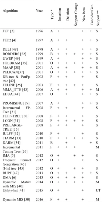
Dynamic itemset mining algorithms introduced so far achieve some level of dynamicity with different interests. Characteristics of twenty seven different algorithms are compared in Table 4. The type of the algorithm is indicated in the third column as follows. “A” means that algorithm is Apriori based; “F” indicates that algorithm is FP-Growth algorithm based; “B” presents that algorithm uses Border based approach and “O” indicates that algorithm uses other data structures like tries and matrices. Columns 4-7 indicate attributes corresponding to the behavior of the algorithm in handling insertions and deletions in the updates, permitting support change and new items in the increments. 8th column shows if the algorithm works with or without candidate itemsets generation in the itemset mining process. The last column shows if the algorithm handles single or multiple support thresholds.

The first group of dynamic algorithms is represented with “A” in the third column of Table 4, uses apriori property and employs iterative level wise search. Since these algorithms are Apriori based, candidate generation and scanning the original database several times in some cases are the major disadvantages in terms of running time performance. Another disadvantage is that the

Figure 13: D1 (Retail)–addition Figure 14: D2 (T40i10d100K)–addition Figure 15: D4 (Kosarak)–addition

(7)

second group of dynamic algorithms is based on the FP-Growth Algorithm is presented by “F” in the third column of Table 4. All algorithms of this group handle single support threshold except the algorithmin Incremental Tuning Tree [26] and Dynamic MIS [50].

Table 4: Dynamic frequent pattern algorithms

*Type: A: Apriori, F: FP-Growth, B: Border, O: Other data structures **Support: S: Single Support, M: Multiple Support, UT: Utility

The third group of dynamic algorithms shown with “B” in the third column of Table 4, is based on the notion of border theory. The Dynamic Borders Algorithm [22] works by constantly maintaining the count information for all frequent and border sets in the current relation. When an increment arrives, the update is

sets. Additional scans of the entire relation are performed only if the support of some border set has reached the minimum support threshold. There are two algorithms that are border based, BORDERS [22] and DARM [34]. The last one is for deletion only and does not allow support change. Both algorithms handle single support threshold. The last group presents algorithms that use different data structures to maintain up-to-date itemsets and are shown with “O” in the third column of Table 4. Most of them are for single support threshold except Dynamic Matrix with MIS [40] that handles multiple support thresholds and the last one handles utility thresholds Utility-list [41].

5 CONCLUSION

This study focuses on dynamic update problem of frequent itemsets under multiple support thresholds; the challenge is to mine frequent itemsets under multiple support thresholds. In this study, a new dynamic itemset mining under multiple support thresholds algorithm which is called Dynamic CFP-Growth++ is introduced and explained, it is tree based, scans the databases only once and avoids the candidate generation problem. It handles increments of additions, additions with new items and deletions. Proposed algorithm is compared to Dynamic MIS [50] and CFP-Growth++ [2] algorithms which are able to find frequent itemsets under multiple support thresholds in dynamic and static databases respectively.

In the performance evaluation work, it is observed that in dynamic database, both of the dynamic algorithms are better than the static algorithm CFP-Growth++, since they run only for the increments, while the static algorithm run from the scratch. It is found out that Dynamic CFP-Growth++ performs better than Dynamic MIS in terms of memory usage since Dynamic MIS algorithm keeps the whole tree in memory without any compacting. As execution time performance; Dynamic MIS is better than Dynamic Growth++ since Dynamic CFP-Growth++ loses time in compacting the tree using pruning and merging procedures that have high complexities and as a result they need more execution time. As it is observed from the experiments, Dynamic CFP-Growth++ and Dynamic MIS have a trade-off relationship in terms of memory usage and execution time.

ACKNOWLEDGMENTS

This work is partially supported by the Scientific and Technological Research Council of Turkey (TUBITAK) under ARDEB 3501 Project No: 114E779. The authors would like to thank Sadeq Darrab for converting the code of CFP-Growth++ algorithm [2].

REFERENCES

[1] Y. Hu and Y. Chen. 2006. Mining association rules with multiple minimum supports: a new mining algorithm and a support tuning mechanism. Decision Support Systems, 42(1), 1–24.

[2] R. U. Kiran and P. K. Reddy. 2011. Novel Techniques to Reduce Search Space in Multiple Minimum Supports-Based Frequent Pattern Mining Algorithms. In The 14th International Conference on Extending Database Technology, ACM, New York, USA, 11–20.

[3] D. W. Cheung, J. Han, V.T. Ng, and C.Y. Wong. 1996. Maintenance of discovered association rules in large databases. An incremental updating technique, In the 12th IEEE International Conference on Data Engineering, Upsala, Sweden, 106–114.

[4] D. W. Cheung, S. D. Lee, and B. Kao. 1997. A general incremental technique for maintaining discovered association rules. In the 5th International Conference on Database Systems for Advanced Applications, Melbourne,

Algorithm Year Type * In ser tio n Deletio n Suppor t C ha nge New I tem Can did ateGen . Suppor t ** FUP [3] 1996 A + + + S FUP2 [4] 1997 A + + + + S DELI [48] 1998 A + + + + S BORDERS [22] 1999 B + + + + + S UWEP [49] 1999 A + + + S FOLDRAM [35] 2001 O + + + + S MAAP [38] 2001 A + + + + S PELICAN[37] 2001 O + + + + + S

DB-tree &

PotFp-tree [42] 2002 F + + + S FELINE [25] 2003 F + + + + S MMA_ITTE [43] 2006 A + + + + M EDUA [44] 2007 O + + + S PROMISING [39] 2007 A + + + S Incremental FP-Tree [31] 2008 F + + + S FUFP-TREE [30] 2008 F + + + S I-CON [31] 2008 F + + + + S PRELARGE-TREE [36] 2008 F + + + S IULFP [32] 2010 F + + S TIARM [33] 2010 F + + + + S DARM [34] 2011 B + + S Incremental Tuning Tree [26] 2011 F + + + M IMA [5] 2012 O + + + S Frequent Itemset Generation [46] 2012 O + + S (I-Is) tree [45] 2012 O + + + S RUPF [47] 2013 O + + + + S DMA [6] 2013 O + + + + S Dynamic Matrix with MIS [40] 2014 O + + + + M Utility-list [41] 2015 O + + UT Dynamic MIS [50] 2016 F + + + M

(8)

Australia, 185–194.

[5] D. Oğuz and B. Ergenç. 2012. Incremental Itemset Mining Based on Matrix Apriori. In DaWaK'12 Proceedings of the 14th international conference on Data Warehousing and Knowledge Discovery, Vienna, Austria, 192–204.

[6] D. Oğuz, B. Yıldız, and B. Ergenç. 2013. Matrix-Based Dynamic Itemset Mining Algorithm. International Journal of Data Warehousing and Mining, 9(4), 62–75.

[7] R. Agrawal, T. Imielinski, and A. Swami. 1993. Mining association rules between sets of items in large databases. In ACM SIGMOD international conference on Management of data, Washington DC, 207–216.

[8] R. Agrawal and R. Srikant. 1994. Fast algorithms for mining association rules in large databases. In the 20th International Conference on Very Large Data Bases, San Francisco, CA, 487–499.

[9] J. Han, J. Pei, and Y. Yin. 2000. Mining frequent patterns without candidate generation. In ACM SIGMOD International Conference on Management of Data, ACM New York, 1–12.

[10] J. Pavon, S. Viana, and S. Gomez. 2006. Matrix Apriori: Speeding up the search for frequent patterns. In the 24th IASTED International Conference on Database and Applications, Innsbruck, Austria, 75–82.

[11] B. Yıldız and B. Ergenç. 2010. Comparison of Two Association Rule Mining

Algorithms without Candidate Generation. In the 10th IASTED International Conference on Artificial Intelligence and Applications, Innsbruck, Austria, 450–457.

[12] B. Liu, W. Hsu, and Y. Ma. 1999. Mining association rules with multiple minimum supports. In the 5th ACM SIGKDD International Conference on KDD, San Diego, CA, 337–341.

[13] H. Mannila. 1998. Database methods for data mining. Tutorial notes, the 4th ACM SIGKDD International Conference on KDD, Technical report, AAAI, Menlo Park, CA.

[14] M. Chen, J. Han, and P. S. Yu. 1996. Data mining: An overview from a database perspective. IEEE Transaction on knowledge and Data Engineering, 8(6), 866–883.

[15] H. Mannila, H. Toivonen, and A. I. Verkamo. 1994. Efficient algorithms for discovering association rules. In AAAI Workshop on KDD, Seattle, WA, 181– 192.

[16] R. Agrawal, H. Mannila, R. Srikant, H. Toivonen, and A. I. Verkamo. 1996. Fast discovery of association rules. In Advances in KDD. MIT Press, 12(1), 307–328.

[17] A. Savasere, E. Omiecinski, and S. B. Navathe. 1995. An efficient algorithm for mining association rules in large databases. In the 21st VLDB Conference, Zurich, Switzerland, 432–443.

[18] J. S. Park, M. Chen, and P. S. Yu. 1995. An effective hash-based algorithm for mining association rules. In ACM SIGMOD International Conference on Management of Data, San Jose, CA, 175–186.

[19] R. Srikant, Q. Vu, and R. Agrawal. 1997. Mining association rules with item constraints. In ACM KDD International Conference, Newport Beach, CA, 67– 73.

[20] R. T. Ng, L. V. S. Lakshmanan, J. Han, and A. Pang. 1998. Exploratory mining and pruning optimizations of constrained associations rules. In ACM-SIGMOD International Conference on Management of Data, Seattle, WA, 13–24. [21] G. Grahne, L. Lakshmanan, and X. Wang. 2000. Efficient mining of

constrained correlated sets. In the 16th International Conference on Data Engineering, San Diego, CA, 512–521.

[22] Y. Aumann, R. Feldman, O. Lipshtat, and H. Manilla. 1999. Borders: An efficient algorithm for association generation in dynamic databases. Journal of Intelligent Information System, 12(1), 61–73.

[23] S. Shan, X. Wang, and M. Sui. 2010. Mining Association Rules: A continuous incremental updating technique. In: International Conference on WISM, IEEE Computer Society, Sanya, China, 62–66.

[24] B. Dai and P. Lin. 2009. iTM: An Efficient algorithm for frequent pattern mining in the incremental database without rescanning. In the 22nd International Conference on Industrial, Engineering and Other Applications of Applied Intelligent Systems, Tainan, Taiwan, 757–766.

[25] W. Cheung and O. R. Zaiane. 2003. Incremental mining of frequent patterns without candidate generation or support constraint. In IDEAS, Hong Kong, China, 111–116.

[26] F. A. Hoque, M. Debnath, N. Easmin, and K. Rashad. 2011. Frequent Pattern mining for multiple minimum supports with support tuning and tree maintenance on incremental database. Research Journal of Information Technology, 3(2), 79–90.

[27] J. Han, M. Kamber, and J. Pei. 2006. Data mining concepts and techniques. Morgan Kaufmann Publishers, Location-Based Services Jochen Schiller, Agnes Voisard, 157–218.

[28] Frequent Itemset Mining Implementations Repository, http://fimi.ua.ac.be/data/ [29] S. Darrab and B. Ergenç. 2016. Frequent pattern mining under multiple support thresholds. In: The 16th Applied Computer Science Conference, Wseas Transactions on Computer Research, Istanbul, Turkey, 4, 1–10.

[30] T. Hong, C. Lin, and Y. Wu. 2008. Incrementally fast updated frequent pattern trees. Expert Systems with Applications, 4(34), 2424–2435.

[31] M, R. Alhajj, and K. Barker. 2008. Alternative method for incrementally constructing the FP-Tree. Studies in Computational Intelligence 109, 361–377. [32] T. Li and X. Li. 2010. An efficient incremental updating algorithm based on

LFP-tree for mining association rules. In Proceedings of the International Conference on Computer Application and System Modeling, Taiyuan, China, 426–430.

[33] G. Pradeepini, S. Jyothi. 2010. Tree-based in¬cremental association rule mining without candidate itemset generation. In Proceedings of the Conference on Trendz in Information Sciences & Computing, Chennai, India, 78–81. [34] M. Taha, T. Gharib, and H. Nassar. 2011. DARM: Decremental association

rules mining. Journal of Intelligent Learning Systems and Applications 3(3), 181–189.

[35] Y. Woon, W. Ng, and A. Das. 2001. Fast online dynamic association rule mining. In Proceedings of the 2nd International Conference on Web Information Systems Engineering, 278–287.

[36] C. Lin, T. Hong, W. Lu, and B. Chien. 2008. Incremental mining with prelarge trees. In Proceedings of the 21st International Conference on Industrial, Engineering and Other Applications of Applied Intelligent Systems, Wroclaw, Poland, 169–178.

[37] A. Veloso, B. Possas, W. M. Jr., and M. B. de Carvalho. 2001. Knowledge management in association rule mining. Workshop on Integrating Data Mining and Knowledge Management, held in conjuction with IEE International Conference on Data Mining.

[38] Z. Zhou and C. I. Ezeife. 2001. A low-scan incremental association rule maintenance method. In Proceedings of the 14th Canadian Conference on Artificial Intelligence, Ottawa.

[39] R. Amornchewin and W. Kreesuradej. 2007. Incremental association rule mining using promising frequent itemset algorithm. In Proceedings of the 6th International Conference on Information, Com¬munications and Signal Processing, Singapore.

[40] V. Chaudhary. 2014. Multiple Minimum Support Implementations with Dynamic Matrix Apriori Algorithm For Efficient Mining of Association Rules. International journal for Scientific Research and Development 2(7), 489 –500. [41] J. C. Lin, W. Gan, T. Hong, and B. Zhang. 2015. An incremental high-utility

mining algorithm with transaction insertion. The Scientific World Journal. [42] C. Ezeife, Y. Su. 2002. Mining incremental association rules with generalized

FP-tree. Proceedings of the 15th Conference of the Canadian Society for Computational Studies of Intelligence on Advances in Artificial Intelligence, Calgary, Canada, 147–160.

[43] M. Tseng, W. Lin, and R. Jeng. 2006. Incremental maintenance of generalized multi-supported association rules under transaction update and taxonomy evolution. In IEEE International Conference on Systems, Man and Cybernetics, Taipei, Taiwan, 2142–2147.

[44] S. Zhang, J. Zhang, and C. Zhang. 2007. EDUA: An efficient algorithm for dynamic database mining. Information Sciences 177(13), 1–12.

[45] P. Vispute and S. Sane. 2012. Incremental learning algorithm for association rule mining. International Journal of Scientific and Engineering Research 3(11), 1–5.

[46] R. Y. Ajay, S. Kumar, P. Kumar, and R. M. Pai. 2012. An improved frequent itemset generation algorithm based on correspondence, Computer Science and Information Technology 2(5), 253–258.

[47] A. Mundra, P. Tomar, and D. Kulhare. 2013. Rapid Update in Frequent Pattern form Large Dynamic Database to Increase Scalability. International Journal of Soft Computing and Engineering 2(6), 307– 310.

[48] S. D. Lee, D. W. Cheung, and B. Kao. 1998. Is sampling useful in data mining? A case in the maintenance of discovered association rules. Data mining and Knowledge Discovery 2(3), 233– 262.

[49] N. Ayan, A. Tansel, and M. Arkun. 1999. An efficient algorithm to update large itemsets with early pruning. In Proceedings of the Fifth ACM SIGKDD International Conference on Knowledge Discovery and Data Mining, San Diego, CA, 287–291.

[50] N. Abuzayed and B. Ergenç. 2016. Dynamic itemset mining under multiple support thresholds. 2nd International Conference on Fuzzy Systems and Data Mining, China Macau, 11-14.