Direct numerical simulation of a NACA0012 in full stall
I. Rodr´ıgueza, O. Lehmkuhla,b, R. Borrellb, A. Olivaa,∗
aCentre Tecnol`ogic de Transfer`encia de Calor, Universitat Polit`ecnica de Catalunya,ETSEIAT, Colom 11,
08222 Terrassa (Barcelona), Spain.
bTermo Fluids, S.L., Avda. Jaquard, 97 1-E, 08222 Terrassa (Barcelona), Spain
Abstract
This work aims at investigating the mechanisms of separation and the transition to turbulence in the separated shear-layer of aerodynamic profiles, while at the same time to gain insight into coherent structures formed in the separated zone at low-to-moderate Reynolds numbers. To do this, direct numerical simulations of the flow past a NACA0012 airfoil at Reynolds numbers Re = 50000 (based on the free-stream velocity and the airfoil chord) and angles of attack AOA = 9.25◦ and AOA = 12◦ have been carried out. At low-to-moderate Reynolds numbers, NACA0012 exhibits a combination of leading-edge/trailing-edge stall which causes the massive separation of the flow on the suction side of the airfoil. The initially laminar shear layer undergoes transition to turbulence and vortices formed are shed forming a von K´arm´an like vortex street in the airfoil wake. The main characteristics of this flow together with its main features, including power spectra of a set of selected monitoring probes at different positions on the suction side and in the wake of the airfoil are provided and discussed in detail.
Keywords: DNS, stall, coherent structures, vortex shedding
1. Introduction
Stall on airfoils is caused by the massive separation of the flow, which deteriorates their performance leading to a sharp drop in the lift and an increase in the drag over the airfoil surface. According to Gregory and O’Reilly (1973), the NACA0012 airfoil exhibits two types of stall: i) a trailing-edge stall at all Reynolds numbers and, ii) a combined leading-edge/trailing-edge stall at intermediate Reynolds number. The latter is characterised by the presence of a turbulent boundary layer separation moving forward from the trailing-edge as the angle of attack (AOA) increases and, a small laminar bubble in the leading-edge region failing to reattach. The combination of these two mechanisms complete the flow breakdown. An oscillating situation is
∗Tel: +34 93 739 8192; fax: +34 93 739 8101
Email address: [email protected]( A. Oliva)
*Manuscript
often noticed near stall angles (see for instance Broeren and Bragg (1999); Rinoie and Takemura (2004); Almutairi et al. (2010)).
The flow around airfoils in full stall is a problem of great interest in aerodynamics and specif-ically for the design of turbo-machines (turbines, propellers, wind turbines, etc.). Indeed, it is a complex flow phenomena which involves separation of the flow from the leading edge, transition to turbulence in the separated shear layer and the shedding of vortices. This vortex shedding is also the cause of strong fluctuations in the lift and drag. It was shown by Broeren and Bragg (1998) that depending on the stall type, these unsteady effects might be of different amplitude, the most severe ones are those encountered in the thin-airfoil/trailing-edge stall type. However, mechanisms of quasi-periodic oscillation observed near stall and stall behaviour, which affect airfoil efficiency, remain still not fully understood. Thus, the study of the separation mechanism and boundary layer transition are both key aspects for improving engineering designs.
The development of coherent structures in the wake of airfoils and transition to turbulence in the separated shear-layer have been object of different studies. For instance, Huang and Lin (1995) and Lee and Huang (1998) studied the flow patterns and characteristics of the vortex shedding of a NACA0012 airfoil. They identified four different modes of vortex shedding: lam-inar, subcritical, transitional and supercritical. According to these studies, in the transitional mode the flow is less coherent, the wake structure is disorganised and no vortex shedding fre-quency can be identified. In addition, Huang and Lin (1995) measured the vortex shedding frequency in the range of Reynolds numbers of 2.5×10⁴ - 1.2×10⁵, and observed that for angles of attack larger than 15◦ this frequency gradually converges to a value of 0.12 as the AOA approaches to 90◦. More recently, Yarusevych et al. (2009) studied experimentally the development of the coherent structures in the separated shear layer of a NACA0025 at low-to-moderate Reynolds numbers in the range 5.5×10⁴ - 2.1×10⁵. They provided some insight into the structures formed and, also measured both the shear-layer instability and vortex shedding frequencies for low AOA. Later, Yarusevych et al. (2011) investigated the vortex shedding char-acteristics of a NACA0018 at low Reynolds numbers. They found that vortex shedding occurs at both flow regimes, i.e. when there is laminar separation with and without flow reattachment. However, although some similarities in the flow can be observed with a NACA0012, there are also important differences as the type of stall these airfoils experience, which is different than that observed in NACA0012.
In addition to experimental studies, the advances in computational fluid dynamics together with the increasing capacity of parallel computers have made possible to tackle complex
tur-bulent problems by using high-performance numerical techniques such as direct numerical sim-ulation (DNS) (Lehmkuhl et al., 2011; Rodr´ıguez et al., 2011a, 2012). DNS has a key role for improving the understanding of the turbulence phenomena and for the simulation of transi-tional flows in complex geometries. In the present work DNS of the flow past a NACA0012 airfoil at low-to-moderate Reynolds number of Re= 5×10⁴ and angles of attack of 9.25◦ and 12◦ (the last one correspond to a full-stall situation) have been carried out. This work aims at investigating the mechanisms of separation and transition to turbulence in the separated shear-layer, while at the same time to gain insight into the coherent structures formed in the separated zone at low-to-moderate Reynolds numbers. The main features of the flow, including power spectra of a set of selected monitoring probes at different positions in the suction side and in the near-wake of the airfoil, are discussed in detail.
2. Mathematical and numerical method
The incompressible Navier-Stokes equations can be written as
Mu = 0 (1)
∂u
∂t +C(u)u+νDu+ρ−1Gp = 0 (2)
where u and p are the velocity vector and pressure, respectively; ν is the kinematic viscosity and ρ the density. Convective and diffusive terms in the momentum equation for the velocity field are given by C(u) = (u· ∇) and D = −∇2 respectively. Gradient and divergence (of a vector) operators are given by G=∇ and M =∇·, respectively.
The governing equations have been discretised on a collocated unstructured grid arrange-ment by means of second-order conservative schemes (Verstappen and Veldman, 2003). Such schemes preserve not only mass and momentum, but also the kinetic energy balance. To con-serve these balances, discrete operators should have the same properties of the continuous ones, i.e. the convective operator should be skew-symmetric (C(u) = −C∗(u)); the negative con-jugate transpose of the discrete gradient operator should exactly be equal to the divergence operator (−(ΩG)∗ = M) and, the diffusive operator (D) should be symmetric and positive-definite. Furthermore, if these properties are preserved, stability at high Reynolds numbers even with coarse grids is ensured.
algorithm should be capable of solving all temporal scales while, at the same time, it should be kept within the stability domain. Different temporal schemes have been proposed in the literature to deal with time marching algorithm for turbulent flows (see for instance Le and Moin (1991); Kim and Choi (2000); Fishpool and Leschziner (2009)). In this work, a two-step linear explicit scheme on a fractional-step method proposed by Trias and Lehmkuhl (2011) has been used. Its main advantage relies on its capacity of dynamically adapt the time step to the maximum possible value, while at the same time it is kept within the stability limits. This strategy reduces the computational time required without lost of accuracy. The method has been successfully tested in different flows in Trias et al. (2010); Rodr´ıguez et al. (2012); Jaramillo et al. (2012).
As aforementioned, the classical fractional step projection method has been used for solving the velocity-pressure coupling,
up =un+1+Gp˜ (3)
where ˜p=pn+1Δtn/ρ is the pseudo-pressure, up the predicted velocity, n+ 1 is the instant where the temporal variables are calculated, andΔtn is the current time step (Δtn=tn+1−tn). Taking the divergence of (3) and applying the incompressibility condition, yields a discrete Pois-son equation for ˜p: Lp˜=Mup. The discrete laplacian operator L ∈Rm×m is, by construction, a symmetric positive definite matrix (L ≡MΩ−1M∗). Once the solution of pn+1 is obtained, ˜p results from equation 3.
Finally the mass-conserving velocity at the faces (Mfunf+1 = 0) is obtained from the cor-rection, unf+1 =upf −Gf˜p, where Gf represents the discrete gradient operator at the CV faces (here the subscript f applies for the faces of the CVs). This approximation allows to conserve mass at the faces but it has several implications. If the conservative term is computed using un+1
f , in practice an additional term proportional to the third-order derivative of pn+1 is
intro-duced. Thus, in many aspects, this approach is similar to the popular Rhie and Chow (1983) interpolation method and eliminates checkerboard modes.
When the fractional step method on a collocated arrange is used, the kinetic energy balance is not strictly ensured. This issue was shown for finite-difference schemes by Morinishi et al. (1998) and for finite-volume schemes by Felten and Lund (2006). The sources of these inac-curacies are two: i) due to interpolation schemes and, ii) due to inconsistency in the pressure field in order to ensure mass conservation. While the first one can be eliminated through the use of conservative schemes such as those used in the present work, the total contribution of
the pressure gradient term to the evolution of the kinetic energy yields,
ke = (˜p)∗M(G−Gf)˜p (4)
This contribution of the pressure gradient term to the evolution of the kinetic energy can not be eliminated. Felten and Lund (2006) conducted an analytical study to determine the scaling order of these errors. They shown that the spatial term of the pressure error scales as O(Δx2) and the temporal term scales as O(Δt2), i.e. pressure errors are of the order of O(Δx2 Δt2). As was suggested in their work, these errors are not of importance with the grid sizes (h) and time-steps (Δt) used in DNS and well-solved large-eddy simulations. In those cases, the own requirements of solving well all spatial and temporal scales of the flow are restrictive enough and thus, the impact of pressure errors should be minimal. The methodology used in this work have been proven to yield accurate results and have been previously used for solving the flow over bluff bodies with massive separation in Rodr´ıguez et al. (2011a,b, 2012).
2.1. Definition of the case. Geometry and boundary conditions.
Direct numerical simulations of the flow past a NACA0012 at Reynolds number of Re = UrefC/ν = 5×10⁴ and AOA= 9.25◦ and 12◦ are considered. Here Reynolds number is defined
in terms of the free-stream velocityUref and the airfoil chordC. All computed flows are around a NACA0012 airfoil extended to include sharp trailing edge. All coordinates are referred to body axes unless remarked. The xaxis is chord-wise, yis in the plane of the airfoil andz is spanwise direction. Solutions are obtained in a computational domain of dimensions 40C×40C×0.2C with the leading edge of the airfoil placed at (0,0,0) (see figure 1). Distances from the profile to the domain boundaries have been chosen according to previous experiences and potential vortices notions (Baez et al., 2011; Lehmkuhl et al., 2011). The boundary conditions at the inflow consist of a uniform velocity profile (u,v,w)=(UrefcosAOA, UrefsinAOA,0). As for the outflow boundary, a pressure-based condition is imposed. No-slip conditions on the airfoil surface are prescribed. Periodic boundary conditions are used in the spanwise direction.
2.2. Computational details
The resolution of the Poisson equation derived from the incompressibility constrain is the main bottleneck from the computational point of view. This can be circumvented by using a Fast Fourier Transform (FFT) based algorithm (Swarztrauber, 1977; Soria et al., 2002). The present method takes the advantage of the mesh discretization, which is obtained from
Figure 1: Computational domain (not-to-scale). Grey dashed line represents inflow conditions, with specified velocity and pressure. Grey solid line represents outflow condition.
the constant step extrusion of a two-dimensional (2D) unstructured grid. By doing this, the spanwise coupling of the discrete Poisson equation results into circulant sub-matrices that are diagonalizable in a Fourier space (Davis, 1979; Gray, 2006), allowing the use of FFT method. This diagonalization decouples the initial three-dimensional (3D) system into a set of mutually uncoupled 2D subsystems which can be solved by means of a Direct Schur-complement based Decomposition method (DSD). The main drawbacks of such algorithm are the requirement of a computationally demanding pre-processing stage and large memory resources. However, this additional pre-processing cost becomes almost negligible compared to the total time-integration cost. For more details the reader is referred to Borrell et al. (2011).
For the meshes reported in the present work, parallelisation strategies have considered parti-tions of 320 CPUs. The computaparti-tions have been carried out on a 76 nodes in-house cluster, each node has 2 AMD Opteron 2350 Quad Core processors linked with an infiniband DDR4 network, and on MareNostrum supercomputer at the Barcelona Supercomputing Center (BSC). When these computations have been performed, MareNostrum supercomputer was an IBM Blade-Center JS21 Cluster with 10 240 PowerPC 970MP processors at 2.3 GHz with 1 MB cache per processor. Quad-core nodes with 8 GB RAM were coupled by means of a high-performance Myrinet network.
2.3. Numerical domain. Mesh resolution studies.
For carrying out the computations at both AOA (AOA = 9.25◦ and AOA = 12◦) two different grids have been used. The grids used are unstructured, which allow to have a good resolution in the zones where the flow is turbulent, while at the same time a coarser mesh is used in the zone where the flow is less complex (i.e. laminar zones). In the construction of these computational meshes, they have been adapted to the different AOAs. Furthermore, it has been considered that the flow around the airfoil is mostly laminar with the exception of a zone close to its surface (suction side) and in the wake of it. In these zones, where the flow is turbulent, the grid size should be enough for solving well the smallest flow scales. Moreover, within laminar zones, boundary layer must also be well-solved. Taking into account that the accuracy of the results is highly grid dependent, specially in the region of the separated shear-layer where transition to turbulence occurs, care must be taken when the computational grid is constructed. Another critical region is the near wake of the airfoil, where a poor grid resolution may cause notable upstream flow distortions. With these criteria, control volumes have been clustered in these zones. Even though the grids used are unstructured, in order to avoid spurious solutions they have been constructed as uniform as possible in the regions of interest. The results presented in the paper have been performed on grids of about 46.6 million CVs (340526 ×128 planes) and 49 MCVs (381762 ×128 planes) for AOA = 9.25 and 12◦, respectively. An example of one of the 2D grid used and its refinement around the suction side of the airfoil is depicted in figure 2.
The quality of the grid resolution used in the present computations has been assessed by means ofa-posteriori analysis of the zones off the wall. To do this, the grid sizeh(h≡(ΩCV)1/3) has been compared to the Kolmogorov length scale η. The Kolmogorov length scale has been obtained from the dissipation rate as,
η= (ν3/)1/4 (5)
where the turbulent kinetic energy dissipation rate can be evaluated as = 2νSij Sij , beingSij the mean rate-of-strain fluctuations.
Figure 3 shows the ratio h/η for different locations in the suction side for both AOA. As can be seen from the figure, this ratio has been kept lower than the unity for most of the region compressed in the turbulent detached zone and the near wake. Indeed, the average value of this ratio for AOA = 9.25◦ in the suction side up to y/C ∼ 0.5 and in the near wake up to
x/C ∼3 has been abouth/η ≈0.389. ForAOA= 12◦, this ratio has been slightly larger, being of h/η ≈ 0.498. With these considerations, the grid densities obtained should be fine enough to solve the smallest flow scales in the zones of interest at this Reynolds number.
The resolution of the grid in the near-wall region has also been assessed by evaluating the grid size in the cells adjacent to the airfoil surface in wall-units. Being the friction velocity uτ = (τw/ρ), the distance from the wall measured in viscous length can be evaluated as
y+ = u
τy/ν. In a similar manner the streamwise Δx+ and spanwise Δz+ cell sizes can be
obtained. The near-wall grid resolution obtained with for AOA = 12◦ is plotted in figure 4. As can be seen from the figure, wall resolution seems to be sufficiently fine for carrying out the present computations.
Regarding the spanwise size of the domain, it has been fixed to 20% of the chord, similar to the values adopted by other investigations at comparable Reynolds numbers (You et al., 2008; Zhou and Wang, 2011). However, in order to verify if this size is adequate, spanwise two-point correlations have been computed. These correlations give an indication of the size of the flow structures in this direction. Thus, the domain should be considered wide enough if their values tend to zero as they approach to the half-size of the domain. Two-point correlations are defined as, ii(x, δz) = < u i(x, t)ui(x+δz, t)> < u2 i > (6) where x≡ (x, y, z) and <·> denotes averaging over time and space. In order to calculate two-point correlations at different locations, the time signals of different stations on the suction side have been recorded. The location of these probes are given in figure 5. The computed values for the stream-wise velocity fluctuations (Ruu) for AOA= 12◦, are given in figure 6. As can be observed, Ruu at the different stations vanishes at the half-width of the domain. In the figure can also be seen the average size of stream-wise structures at the different locations, as the position of the minimum denotes the mean distance between a high and a low-speed flow structure. Thus, the size of these structures is twice this distance. Considering these results, the value of 20% of the chord is good enough for capturing the largest scales of the flow.
3. Results
For obtaining the numerical results presented, the simulations have been started from an initially homogeneous flow field which introduces some numerical disturbances as it is not the solution of the governing equations. These disturbances eventually cause the flow became
0 0.1 0.2 0.3 0.5 1 y/c x/c=0.3 h/η 0.5 1 x/c=0.6 0.5 1 x/c=0.8 0.5 1 x/c=0.95 0.5 1 x/c=2 (a) 0 0.1 0.2 0.3 0.5 1 y/c x/c=0.3 h/η 0.5 1 x/c=0.6 0.5 1 x/c=0.8 0.5 1 x/c=0.95 0.5 1 x/c=2 (b)
Figure 3: Ratio of the grid size to the Kolmogorov length scale at different locations. a)AOA= 9.25◦;
0 2 4 6 8 10 12 14 16 18 20 0 0.1 0.2 0.3 0.4 0.5 0.6 0.7 0.8 0.9 1 x/C y+ Dz+ Dx+
Figure 4: Mesh resolution near the wall obtained for AOA= 12◦
Figure 5: Location of the computational probes
dimensional and trigger the transition to turbulence. Then, simulations have been advanced in time until statistical stationary flow conditions have been achieved and the initial transient has been completely washed out.
3.1. Instantaneous flow structures
In order to gain insight into the coherent structures developed in the separated zone, the
Q-criterion proposed by Hunt et al. (1988) has been used. This method, which is based on the second invariant of the velocity gradient tensor, defines an eddy-structure as a region with positive second invariant Q. Being the rate-of-strain (S) and the rate-of-rotation (Ω) the symmetric and skew-symmetric components of the velocity gradient tensor ∇u, its second invariant is,
Q= 1
2(Ω
2 − S 2) (7)
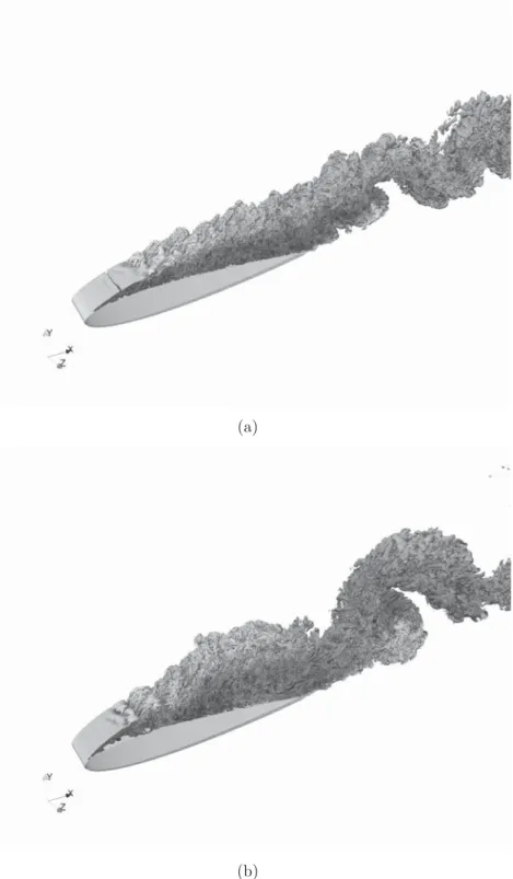
where · denotes the trace of the tensor. Thus, according with the Q-criterion, a region with positiveQis a region where rotation overcomes the strain. Qiso-surface plots are depicted in figure 7. A first inspection to the figure reveal the large quantity of small scales in the separated zone. In fact as the AOA increases one can note how this region is broadened due to the increase of the adverse pressure gradient.
At both AOAs, the flow separates laminarly from the airfoil surface near the leading edge, as can be inferred from the two-dimensional shear-layer. Vortex breakdown occurs at the end of the laminar shear-layer as a consequence of the instabilities developed by the action of a Kelvin-Helmholtz mechanism (see figure 8). These instabilities are high frequency fluctuations in the velocity field which grow in magnitude as the distance from the leading edge increases and eventually causes shear layer to roll-up and undergo transition to turbulent flow. For instance, if the flow at AOA= 12◦ is inspected (see figure 7(b)), these instabilities can clearly be seen at the end of the laminar shear-layer. Indeed, the increase in their amplitude until finally transition to turbulence occurs is also well captured in the figure. This mechanism of transition is similar to that observed in shear-layers developed in other bluff bodies such as the flow past a circular cylinder (see for instance Prasad and Williamson (1997)) or the flow past a sphere (Rodr´ıguez et al., 2011a).
At the end of the two-dimensional shear layer, corrugated structures along the homogeneous direction, can also be observed. Although at both AOA these structures are formed, in the plots are more evident atAOA= 12◦. These corrugated structures are related with the formation of
(a)
(b)
Figure 7: Visualisation of instantaneous vortical structures on the suction side of the airfoil by means of
(a) (b)
(c) (d)
Figure 8: Instantaneous flow. (a,c) Pressure and vorticity contours for AOA = 9.25◦. (b,d) Pressure
and vorticity contours for AOA= 12◦
stream-wise vortices (ribs) in the separated zone. After vortex breakdown, small-scale vortices are formed and accumulate into larger structures forming packets. The frequency at which these instabilities develop is much higher than that of the vortex shedding mechanism (see section 3.2). These turbulent vortical packets, eventually grow up as the flow moves downstream. A close-up to the developing flow structures in the separated shear-layer is shown in figure 8 by means of pressure and vorticity isocontours projected into a two-dimensional plane. For both AOA this phenomena can be seen in the figure. The extension of the separated zone increases with the AOA and, at AOA= 12◦ the wake starts within the suction side region. Kelvin-Helmholtz instabilities appear as small vortices in the pressure field at both AOAs. After transition, by means of the pairing of vortices large scale structures are formed. Vortices originated at the trailing edge of the airfoil are also shown. In fact, at AOA = 12◦, these vortices irrupt into the suction side, interacting with those from the suction side, to form a pattern similar to a von K´arm´an like vortex street (not shown here), which resembles that formed behind a circular cylinder.
According to Huang and Lin (1995) observations of the flow past a NACA0012 airfoil at low-to-moderate Reynolds numbers, the way vortices are shed into the wake present four char-acteristics modes: laminar, subcritical, transitional and supercritical. In this characterisation, in the transitional mode vortices shed are irregular and without coherence, forming a disor-ganised wake. They did not detect any vortex shedding in this regime. On the other hand,
(a) (b)
Figure 9: Streamwise velocity time series at P5 station. a) AOA= 9.25◦; b)AOA= 12◦
in the supercritical mode, the flow is coherent and turbulent vortex shedding is re-established. Following Huang and Lin (1995) classification, at AOA = 9.25◦ wake mode should correspond with the transitional one, whereas at AOA = 12◦ supercritical mode should be detected. In fact, from the inspection of time series at P5 station (placed in the near wake at x/C = 1.2; y/X = 0.04), stream-wise velocity exhibits a transitional behaviour characterised by the lost of coherence in the signal, although coherence is recovered after some time (see figure 9(a)). At AOA = 12◦, the stream-wise signal is highly coherent (the vortex shedding frequency can almost be calculated directly from the signal) which agrees well with Huang and Lin (1995) supercritical mode (see figure 9(b)). The signal of the stream-wise velocity fluctuates due to the passing of large-scale vortices, but also the footprint of the small-scale shear layer fluctuations is superimposed. It should be pointed out, that contrary to Huang and Lin (1995) observations, in the present simulations vortex shedding has been detected at AOA = 9.25◦ as is discussed in the next section, being in agreement with the measurements of Yarusevych et al. (2009) for a NACA0025 at low-to-moderate Reynolds numbers.
3.2. Energy spectra
As has been commented before, time series of velocity components and pressure have been recorded on different locations (see figure 5). The data have been collected over 120 time units (tU/C) for both AOAs. The energy spectra have been calculated by using the Lomb periodogram technique and the resulting spectra have also been averaged in the homogeneous direction. Figures 10 and 11 show the energy spectra for both stream-wise and cross-stream velocity fluctuations at the two AOAs. In the figures, the main frequencies of the flow are well captured. For clearness, each spectrum has been shifted and is represented for increasing x/C from bottom to top. The energy spectra exhibit different ranges and fundamental frequencies:
1e-08 1e-06 0.0001 0.01 1 100 10000 1e+06 1e+08 0.001 0.01 0.1 1 10 Euu f -5/3 1e-08 1e-06 0.0001 0.01 1 100 10000 1e+06 1e+08 0.001 0.01 0.1 1 10 100 Evv f -5/3
Figure 10: Energy spectra of the stream-wise and cross-stream velocity fluctuations for AOA = 9.25◦. From
top to bottom, spectra correspond with stations P6, P5, P4,P3, P2, P1, P0 (see figure 5 for details)
from transition to turbulent flow observed in the bottom curve of all figures (corresponding with probe P0), to the regular decay of slope close to −5/3, as the flow approaches the airfoil aft and flows into the wake (e.g. probe P6). The latter is indicative of the presence of an inertial subrange for more than a decade of frequencies.
As for the significant frequencies, the spectrum for P0 shows a broadband peak atfSL = 6.9 (St = fsin(AOA)C/U = 1.109, here Strouhal is based on the airfoil projection on a cross-stream plane) and at fSL = 9.74 (St = 2.025) for AOA = 9.25◦ and AOA = 12◦, respectively. This peak corresponds with the frequency of the shear-layer instabilities and disappears as the flow moves downstream and the separated shear layer becomes turbulent. Note that it has only been well captured by the probe P0 located at (x/C = 0.2;y/C = 0.125) which is close to the separated shear layer at both AOAs.
In addition, the energy spectra also show a peak corresponding with the wake vortex shed-ding at both AOAs. In the case of AOA = 9.25◦, this peak is better detected at probes P5 and P6, which are located in the wake behind the airfoil (see Fig. 5). It should be pointed out that Huang and Lin (1995) did not detected the presence of vortex shedding in the tran-sitional mode. Although energy spectra of the stream-wise velocity fluctuations Euu show a
1e-08 1e-06 0.0001 0.01 1 100 10000 1e+06 1e+08 1e+10 0.001 0.01 0.1 1 10 Euu f -5/3 1e-08 1e-06 0.0001 0.01 1 100 10000 1e+06 1e+08 1e+10 0.001 0.01 0.1 1 10 Evv f -5/3
Figure 11: Energy spectra of the stream-wise and cross-stream velocity fluctuations forAOA= 12◦. From top
to bottom, spectra correspond with stations P6, P5, P4,P3, P2, P1, P0 (see figure 5 for details)
wide range of frequencies at which the energy fluctuates indicating the lost of coherence of the signal, vortex shedding is still detected. Indeed, the energy spectrum of the cross-flow velocity fluctuationsEvv better captures this fundamental frequency atfvs = 1.138 (St = 0.183), as this component is more sensitive to the two-dimensional von K´arm´an-like structures formed in the wake.
Another interesting feature is a period-doubling scenario (see energy spectra of stream-wise and cross-stream fluctuations at P5, figure 10). This process is similar to that observed by Hoarau et al. (2006), but at a much lower Reynolds number. The probe at this station detects both the vortex shedding frequency and its sub-harmonic at 0.5fsl. This double-peak mechanism is produced when vortices shed at the trailing edge interact with those shed at separated shear layer every 2 vortex shedding periods. The asymmetry in the vortex shedding causes the interaction between vortices formed at the leading-edge and the trailing-edge. This might be the reason of the lost of coherence in the signal observed both experimentally and numerically. This, together with the fact that in the experiments only the signal of the streamwise velocity in the near wake was measured, points out the cause of the absence of vortex shedding in the transitional mode in Huang and Lin (1995) work.
0 200 400 600 800 1000 1200 1400 1600 1800 2000 0 0.2 0.4 0.6 0.8 1 1.2 1.4 f fvs=1.13 0.5fvs fm=0.13
Figure 12: Energy spectrum of the lift coefficient forAOA= 9.25◦
Another striking fact is the broadband of low frequencies with a large energy content at this AOA at every station. If the spectrum of the lift coefficient is inspected (see figure 12), one can notice that among all these frequencies, there is a pronounced peak at f = 0.13 (St = 0.021). This extremum is related with the low frequency oscillation mechanism reported at near stall angles (Zaman et al., 1989; Bragg et al., 1996; Rinoie and Takemura, 2004). This low frequency mechanism was reported to occur on thin airfoil and trailing-edge stall types as part of the stall mechanism and was associated with the highly unsteady and oscillating flow near stall. The value of the frequency oscillation measured in the present work is close to that reported in the literature which seems to be about St= 0.02. In this case, this low frequency measured just after stall can be interpreted as a flapping of the shear-layer in the direction normal to the airfoil surface, but even though this flapping movement reduces the height of the separated zone at this AOA, it is not sufficient for causing the reattachment of the flow and the closure of this zone.
Contrary to the behaviour observed at AOA = 9.25◦, at AOA = 12◦ the energy spectra of all probes show a distinguishable peak at fvs = 0.613 (St = 0.127), which corresponds with the vortex-shedding process and its energy content increases as the flow approaches the airfoil aft and flows into the wake. Indeed, the signals of the stream-wise and cross-stream velocities gain coherence as the flow moves downstream.
On the basis of the present analysis, wake vortex shedding is detected at both transitional and supercritical regimes, although at the transitional one it is weaker and not so coherent than in the supercritical regime, mainly due to the fluctuation of the separated zone and the
interaction between leading-edge and trailing-edge vortices. Furthermore, these results show that as the AOA increases the wake vortex shedding frequency decreases, whereas the shear-layer instabilities frequency increases. These trends are in agreement with the observations of Huang and Lin (1995) for a NACA0012 and with those reported by Yarusevych et al. (2009) for a NACA0025.
3.3. Mean aerodynamic coefficients
The pressure distribution on the airfoil surface obtained at both AOA is plotted in figure 13(a). In order to have a more complete picture of the pressure changes taking place at stall angles, the pressure distribution before stall at AOA = 8◦ (Baez et al., 2011) is also plotted. In addition the mean skin friction distribution is given in figure 13(b). Near the leading edge, the pressure gradient causes separation of the boundary layer. This separation point moves towards the leading edge with the increase in the AOA (see also figure 13(b)). Boundary layer separation occurs at x/C = 0.0316 for AOA = 9.25◦ and a little forward at x/C = 0.0164 for AOA = 12◦. When comparing the pressure distribution at AOAs under study with that obtained at pre-stall angle of AOA = 8◦, a strong decrease in the suction pressure peak near the leading edge, which is typical of stalled airfoils, can be observed. The pressure profile at AOA = 9.25◦ exhibits a plateau after the suction peak and a further gradual pressure recovery until reaching the trailing edge. This behaviour is quite different of pre-stall angles in which there is a sudden recovery of the suction pressure. Indeed, at AOA= 9.25◦ pressure behaviour is halfway from the profile obtained in flows with laminar separation bubble and flows with fully separation (e.g. AOA= 12◦). A similar pressure distribution was obtained for Rinoie and Takemura (2004) at Re = 1.3×10⁵ and AOA = 11.5−12◦, just after stall. At AOA = 12◦, a much flatter profile is observed, which is typical of fully stalled airfoils. Near the trailing edge a slight depression is also observed. This is due to the vortex entrainment produced by the formation of a much wider wake in the detached zone and the shedding of vortices at the trailing edge (see section 3.1).
As for the mean skin distribution on the suction side of the airfoil (figure 13(b)), it is in correspondence with the pressure profile measured. For both airfoils, a large reversed flow forming a long bubble in the upper surface is observed. For AOA = 12◦, there is a small recirculation near the leading edge and underneath the large recirculation zone. It is between x/C = 0.127 and x/C = 0.245. The broad recirculation region at this AOA closes near the trailing edge at x/C = 0.954.
-2.5 -2 -1.5 -1 -0.5 0 0.5 1 0 0.2 0.4 0.6 0.8 1 Cp x/C (a) -0.01 -0.005 0 0.005 0.01 0.015 0.02 0.025 0.03 0 0.2 0.4 0.6 0.8 1 Cf x/C (b)
Figure 13: (a) Mean pressure coefficient distribution. (b) Mean skin friction. (squares) AOA = 12◦; (solid
squares)AOA= 9.25◦; (solid circles)AOA= 8 from Baez et al. (2011).
4. Concluding remarks
In the current work the mechanisms of transition at the separated shear-layer of a NACA0012 airfoil atAOA= 9.25◦ andAOA= 12◦have been addressed. The study has been performed by means of the direct numerical simulation of the flow at a low-to-moderate Reynolds number of Re= 50000. To do this, a second-order spectro-consistent scheme on a collocated unstructured grid arrangement has been used for the discretization of the governing equations. All compu-tations have been carried out unstructured meshed generated by the constant step extrusion in the homogeneous direction of a two-dimensional grid.
The main frequencies of the flow at both AOAs have been detected by means of power spectra of several probes located on the suction side and in the near wake. In fact, the probe located near the shear-layer well captured the small-scale shear-layer instabilities frequency. These instabilities can be identified in the spectra as a broad-band peak centred at a frequency of fSL = 6.9 (St = 1.109) and fSL = 9.74 (St = 2.025) at AOA = 9.25◦ and AOA = 12◦, respectively. As a consequence of the growth of these instabilities the shear-layer roll-up and transition to turbulence occurs. The small vortices formed after transition are packet into large-scale structures due to vortex pairing. The transition to turbulence and vortex shedding mechanisms reported are quite similar to those observed in other bluff bodies. Furthermore, in agreement with previous experimental studies in similar aerodynamic bodies, wake vortex shedding decreases with the AOA, while shear-layer instabilities frequency increases.
It has been observed that the separated flow at both AOA is slightly different. Indeed, coherent structures identified have shown that in agreement with the experimental observations of Huang and Lin (1995), the flow at AOA= 12◦ is in the supercritical mode, characterised by the presence of a coherent vortex shedding at fvs = 0.613 (St= 0.127). On the other hand, the
flow at AOA = 9.25◦ has been identified with the transitional mode with a more incoherent shedding of vortices. However, contrary to previous experimental observations, in the present work wake vortex shedding has been captured at fvs = 1.13 (St= 0.183). We suggest that the asymmetric vortex shedding and the interaction between leading-edge and trailing-edge vortices might be the cause of the low level of coherence observed in the vortex shedding at this AOA. In addition, the analysis of the lift coefficient spectrum has shown a pronounced peak at a much lower frequency f = 0.13 (St = 0.021), which has been identified with a flapping movement of the shear layer. This low frequency mechanism is in agreement with previous experimental studies which reported oscillations near stall at St = 0.02.
Acknowledgements
This work has been by financially supported by the “Ministerio de Econom´ıa y Competi-tividad, Secretar´ıa de Estado de Investigaci´on, Desarrollo e Innovaci´on”, Spain (ref. ENE2009-07689 and ENE2010-17801) and by the Collaboration Project between Universidad Polit`ecnica de Catalunya and Termo Fluids S.L.
References
Almutairi, J., Jones, L., Sandham, N., 2010. Intermittent bursting of a laminar separation bubble on an airfoil. AIAA journal 48 (2), 414–426.
Baez, A., Lehmkuhl, O., Rodriguez, I., Perez-Segarra, C., 2011. Direct Numerical Simulation of the turbulent flow around a NACA 0012 airfoil at different angles of attack. In: Proceedings of 24th Conference on Parallel CFD, Barcelona, Spain.
Borrell, R., Lehmkuhl, O., Trias, F., Oliva, A., 2011. Parallel direct poisson solver for discretisa-tions with one fourier diagonalisable direction. Computational Physics 230 (12), 4723–4741. Bragg, M., Heinrich, D., Balow, F., Zaman, K., 1996. Flow oscillation over an airfoil near stall.
AIAA journal 34 (1), 199–201.
Broeren, A., Bragg, M., 1998. Low-frequency flowfield unsteadiness during airfoil stall and the influence of stall type. AIAA Paper, AIAA–98–2517.
Broeren, A., Bragg, M., 1999. Flowfield measurements over an airfoil during natural low-frequency oscillations near stall. AIAA journal 37 (1), 130–132.
Davis, P. J., 1979. Circulant Matrices. Wiley-Interscience, New York.
Felten, F., Lund, T., 2006. Kinetic energy conservation issues associated with the collocated mesh scheme for incompressible flow. Journal of Computational Physics 215 (2), 465–484. Fishpool, G., Leschziner, M., 2009. Stability bounds for explicit fractional-step schemes for the
Navier-Stokes equations at high Reynolds number. Computers and Fluids 38, 1289–1298. Gray, R. M., 2006. Toeplitz and circulant matrices: A review. Foundations and Trends in
Communications and Information Theory 2, 155–239.
Gregory, N., O’Reilly, C., 1973. Low-speed aerodynamic characteristics of a naca 0012 airfoil section, including the effects of upper-surface roughness simulating hoar frost. Tech. Rep. R&M 3726, Ministry of Defence. Aeronautical Research Council, London.
Hoarau, Y., Braza, M., Ventikos, Y., Faghani, D., Oct. 2006. First stages of the transition to turbulence and control in the incompressible detached flow around a NACA0012 wing. International Journal of Heat and Fluid Flow 27 (5), 878–886.
Huang, R. F., Lin, C. H., 1995. Vortex shedding and shear-layer instability of wing at low-Reynolds numbers. AIAA Journal 33 (8), 1398–1403.
Hunt, J., Wray, A., Moin, P., 1988. Eddies, stream and convergence zones in turbulent flows. Tech. Rep. CTR-S88, Center for turbulent research.
Jaramillo, J., Trias, F., Gorobets, A., P´erez-Segarra, C., Oliva, A., 2012. Dns and rans modelling of a turbulent plane impinging jet. International Journal of Heat and Mass Transfer 55 (4), 789 – 801.
Kim, D., Choi, H., 2000. A second-order time-accurate finite volume method for unsteady incompressible flow on hybrid unstructured grids. Journal of Computational Physics 162 (2), 411 – 428.
Le, H., Moin, P., 1991. An improvement of fractional step methods for the incompressible navier-stokes equations. Journal of Computational Physics 92 (2), 369 – 379.
Lee, H. W., Huang, R. F., 1998. Frequency selection of wake flow behind a NACA 0012 wing. Journal of Marine science and technology.
Lehmkuhl, O., Baez, A., Rodr´ıguez, I., Perez-Segarra, C. D., 2011. Direct numerical simulation and Large-Eddy simulations of the turbulent flow around a NACA-0012 airfoil. In: 7th International Conference on Computational Heat and Mass Transfer. pp. 1–8.
Morinishi, Y., Lund, T., Vasilyev, O., Moin, P., 1998. Fully conservative higher order finite difference schemes for incompressible flow. Journal of Computational Physics 143 (1), 90– 124.
Prasad, A., Williamson, C., 1997. The instability of the shear layer separating from a bluff body. Journal of Fluid Mechanics, 375–492.
Rhie, C. M., Chow, W. L., 1983. Numerical study of the turbulent flow past an airfoil with trailing edge separation. AIAA Journal 21, 1525–1532.
Rinoie, K., Takemura, N., 2004. Oscillating behaviour of laminar separation bubble formed on an aerofoil near stall. The aeronautical journal 1 (2816).
Rodr´ıguez, I., Borrell, R., Lehmkuhl, O., P´erez-Segarra, C., Oliva, A., 2011a. Direct Numerical Simulation of the Flow Over a Sphere at Re = 3700. Journal of Fluids Mechanics 679, 263– 287.
Rodr´ıguez, I., Lehmkuhl, O., Borrell, R., Oliva, A., 2012. Flow dynamics in the wake of a sphere at sub-critical Reynolds numbers. Computers & Fluids.
Rodr´ıguez, I., Lehmkuhl, O., Borrell, R., P´erez-Segarra, C., Oliva, A., 2011b. Low-frequency variations in the wake of a circular cylinder at Re = 3900. In: Proceedings of the 13th European Turbulence Conference.
Soria, M., P´erez-Segarra, C., Oliva, A., 2002. A direct parallel algorithm for the efficient solution of the pressure-correction equation of incompressible flow problems using loosely coupled computers. Numerical Heat Transfer, Part B 41 (2), 117–138.
Swarztrauber, P., 1977. The Methods of Cyclic Reduction, Fourier Analysis and the FACR Algorithm for the Discrete Solution of Poisson’s Equation on a Rectangle. SIAM Review 19, 490–501.
Trias, F., Gorobets, A., Soria, M., Oliva, A., 2010. Direct numerical simulation of a differentially heated cavity of aspect ratio 4 with rayleigh numbers up to 1011. part i: Numerical methods and time-averaged flow. International Journal of Heat and Mass Transfer 53 (4), 665 – 673.
Trias, F., Lehmkuhl, O., 2011. A self-adaptive strategy for the time integration of navier-stokes equations. Numerical Heat Transfer. Part B 60 (2), 116–134.
Verstappen, R. W. C. P., Veldman, A. E. P., 2003. Symmetry-Preserving Discretization of Turbulent Flow. Journal of Computational Physics 187, 343–368.
Yarusevych, S., Boutilier, H., S., M., Oct. 2011. Vortex Shedding of an Airfoil at Low Reynolds Numbers. AIAA Journal 49 (10), 2221–2227.
Yarusevych, S., Sullivan, P. E., Kawall, J. G., 2009. On vortex shedding from an airfoil in low-Reynolds-number flows. Journal of Fluid Mechanics 632, 245.
You, D., Ham, F., Moin, P., 2008. Discrete conservation principles in large-eddy simulation with application to separation control over an airfoil. Physics of Fluids 20 (10), 101515. Zaman, K., McKinzie, D., Rumsey, C., 1989. A natural low-frequency oscillation for the flow
over an airfoil near stalling conditions. Journal of Fluid Mechanics 202, 403–442.
Zhou, Y., Wang, Z., 2011. A Low-Frequency Instability/Oscillation near the Airfoil Leading-Edge at Low Reynolds Numbers and Moderate Incidences. In: 20th AIAA Computational Fluid Dynamics Conference. AIAA-2011-3548.