Algebraic Multi-Grid solver for lattice QCD on Exascale hardware: Intel Xeon Phi

(1)

Available online at www.prace-ri.eu

Partnership for Advanced Computing in Europe

Algebraic Multi-Grid solver for lattice QCD on Exascale

hardware: Intel Xeon Phi

A. Abdel-Rehim

aa

_{, G. Koutsou}

a

_{, C. Urbach}

b

a_{Computation Based Science and Technology Research Center, The Cyprus Institute, 20 Konstantinou Kavafi Street}

2121 Aglantzia, Nicosia, Cyprus

b_{Helmholtz Institut f}_ü_{r Strahlen und Kernphysik (Theorie) and Bethe Center for Theoretical Physics, Universit}_ä_{t Bonn, 53115 Bonn,}

Germany Abstract

In this white paper we describe work done on the development of an efficient iterative solver for lattice QCD based on the Algebraic Multi-Grid approach (AMG) within the tmLQCD software suite. This development is aimed at modern computer architectures that will be relevant for the Exa-scale regime, namely multicore processors together with the Intel Xeon Phi co-processor. Because of the complexity of this solver, implementation turned out to take a considerable effort. Fine tuning and optimization will require more work and will be the subject of further investigation. However, the work presented here provides a necessary initial step in this direction.

1. Introduction

Simulations of the theory of the strong nuclear force known as Quantum Chromodynamcis or QCD on the lattice have entered a stage where physical light quark masses, small lattice spacing and large volumes are becoming the norm. This offers the great advantage of directly comparing lattice QCD results to experiment without need to do any extrapolation and also with a much smaller lattice error from finite volume or finite lattice spacing. The main bottleneck of lattice computations is the iterative solver in which we need to solve a large sparse linear system of equations to compute the quark propagator. This is usually the most time consuming part of the calculations spending about 70%-90% of the total computational time. Moreover, as we approach the era of realistic lattice simulations with light masses, small lattice spacing and large volumes, these linear systems tend to be ill-conditioned making the convergence of standard iterative solvers such as Conjugate-Gradient (CG) very slow. This makes these simulations very expensive and it is essential to look for more efficient algorithms. In addition, as we enter the Exa-scale era, it is necessary to adapt these algorithms as much as possible to the underlying hardware. This is usually not an easy or straightforward task.

In this work we focus on a very promising iterative solver that has been found as much faster than standard solvers such as the CG Algorithm. This solver is based on Algebraic Multi-Grid methods (AMG). There are few variants of this algorithm in the literature which share the same main ingredients but differ in some optimization details that also play a role in making the algorithm more efficient. In this work, we will closely follow the implementation described in [1]. To our knowledge, there is no open source implementation of this solver available. In this work such an implementation is done in an open source code within the tmLQCD software suite [2]. This software suite has been developed over the years by the European Twisted Mass Collaboration (ETMC) and is widely used by the ETMC community. Initial implementation of tmLQCD was aimed at a special type of lattice fermions, called Twisted-Mass fermions; however, the code now also includes other types of formulations such as clover fermions. TmLQCD is publically available and could be obtained from github [3]. The library includes codes for performing Hybrid Monte-Carlo simulations as well as computing the quark propagator on background gluon field configurations. An important feature of tmLQCD is that it uses MPI as well as openMP for parallization, making it very suitable for the

(2)

core and Xeon-Phi coprocessor. This whitepaper is organized as follows: first we describe the AMG solver and its implementation in tmLQCD. Then we discuss some issues regarding the implementation for the Xeon Phi. Finally we give some results and conclusions.

2. The AMG Iterative Solver

In lattice QCD computations we need to solve many sparse linear systems of the form Dψi=ηi,i=1,. .,n ₍₁₎

where D is a lattice discretization of the Dirac operator. In the simplest case of Wilson fermions for example, this operator is given by

Dψ(x)=ψ(x)−κ

∑

[

Uμ(x)

(

1−γμ

)

ψ

(

x+eμ

)

+Uμ

−1

(

x−e_μ

₎₍

1+γ_μ

₎

ψ

₍

x−e_μ

₎

]

(2)

where x is a lattice site, k is a quark mass parameter and eμ _{is a unit vector in the}μ _{direction. The}

matrices γμ _{are 4x4 matrices in the spin space and}Uμ _{are 3x3 unitary matrices which represents the}

gluon field at the site x. An algebraic multigrid solver has two main components: a smoother and a coarse grid correction. As a smoother corrector one of the standard Krylov methods is usually used. These methods are efficient in dealing with high modes of the Dirac operator. In the current implementation we use a method based on domain-decomposition called Schwarz Alternating Procedure (SAP). The coarse grid correction deals with the low modes (near kernel modes) of the Dirac operator. In its simplest formulation, the solver consists of a two level approach in which one alternates between the coarse grid and the smoother in what is called a V-cycle. The process however can be bootstrapped and a more complicated multi-level procedure can be implemented. In the current implementation, based on [1], we proceed as follows:

• A set of global orthonormal fields ξi,i=1, ..,Ns _{that approximates the low eigenmodes of}

the Dirac operator are built.

• The whole lattice is divided into disjoint blocks

N

b _.

• The global fields are then broken over these blocks giving a set of fields

ϕ

j

,j=

1,. .

,N

b

∗

N

s

which are also orhtonormalized. These blocked fields will provide the space on which the coarse grid correction is computed.

• The projection of the Dirac operator D onto this deflation subspace is called the little Dirac operator

A

where

A

ij

=

(

ϕ

i

,A

ϕ

j

)

_.

• A left projector

P

L

=

1 −

∑

D

ϕ

i

(

A

−1

)

ij

ϕ

hj.c _{is built.} • Amulti-grid preconditioner is then defined by:

M

MG

=M

SAP

P

L

+

∑

ϕ

i

(

A

−1

)

ij

ϕ

hj.c. ₍₃₎ • This multigrid preconditioner is then used in an outer process such as the Flexible GMRES

solver (FGMRES). 3. AMG in tmLQCD

The AMG solver is implemented and tested for the case of Twisted-Mass fermions with or without a clover term. The implementation required designing a new geometrical construction of the lattice where the local volume of the lattice for each MPI process is divided into non-overlapping blocks. Functions needed to build the little Dirac operator as well as solving the little system are built. In addition, the necessary projectors are implemented. The multigrid solver as described in Equation (3) is finally used as a preconditioner within the Flexible GMRES solver which has also been implemented. The AMG solver has a large set of parameters that need to be carefully selected in order to achieve a good performance. These parameters can be classified into:

(3)

1. Parameters for the solver of the little Dirac operator. 2. Parameters for the FGMRES solver.

3. Parameters for the

M

SAP _solver.

4. Parameters for building the coarse grid correction. 4. AMG for the Xeon Phi

As a first step, the AMG solver could be run natively on the Xeon Phi using openMP which is already implemented in tmLQCD. However, it turned out that large memory is required and only small size problems could be run in this case. Alternatively, the main kernel could be run, namely the Dirac operator, on the Xeon Phi and the rest of the code on the host CPUs. Further optimization and testing will be the subject of future work.

4.1 Vectorization of the Dirac operator

In order to achieve a good performance on the MIC the vectorization capabilities of the wide registers needs to be utilized. These registers allow the operation on 8 double or 16 single precision values simultaneously. Since the main kernel involved in the solver is the Dirac operator, it is beneficial to focus on the vectorization of this kernel. The main operation involved is the multiplication of the 3x3 unitary matrices

U

μ

(

x

)

_{times a 3x1 vector. This data layout doesn't lend itself naturally to the 512 bit}

registers available for vectorization on the MIC. The application of the Dirac operator involves a for loop over the local lattice volume of the MPI process. This loop has eight matrix-vector multiplications (3x3 matrix times a 3x1 vector). In addition, there are operations such as scaling of a vector and adding or subtracting two vectors. These vector operations can be easily vectorized with the 512-bit intrinsics. Schematically, the main loop has the structure

for (x=0; x<V; x++) { //+0 direction

U

0

(

x

)

(

1 −

γ

0

)

ψ

(

x+e

0

)

//-0 direction

U

−01

(

x

−

e

0

)(

1 +γ

0

)

ψ

(

x

−

e

0

)

//+1 direction …... //-3 direction

U

−31

(

x

−

e

3

)(

1 +γ

3

)

ψ

(

x

−

e

3

)

}

After studying different possibilities, we found that the best approach is to pack together the matrices and vectors for four lattice sites. In this cases the for loop will run over V/4 elements. A similar approach that will avoid dealing with complex numbers is to store the real and imaginary parts of matrices and vectors separately. In this case we pack together variables for eight sites and the loop run over V/8 elements. These new layouts will require V to be a multiple of 4 or 8 respectively, a condition that will always be satisfied in practice. A sample code that is based on intrinsics is given in the appendix.

(4)

In the following, we give results for testing the AMG solver as well as some preliminary performance results for the vectorization on the Xeon Phi.

5.1 AMG solver on multi-core machines

We first test the solver on a multi-core machine. The test is performed on a Cray XC30 system. Each compute node has two sockets and each socket has 12 core Intel Ivy Bridge processor at 2.4 GHz. TmLQCD is compiled with the Intel compiler and configured with the options

“./configure --enable-mpi –enable-sse2 --with-mpidimension=4 --with-lapack CC=cc F77=ftn”.

We consider two gauge configurations from the ETMC configuration archive with up, down, strange, and charm sea quarks. The parameters of these configurations and there label in the ETMC database is shown in Table 1.

Label b L/a T/a

aμ

_l

aμ

_σ

aμ

_δ κ

B85.24 1.95 24 48 0.0085 0.135 0.170 0.1612312 D15.48 2.1 48 96 0.0015 0.120 0.1385 0.156361

Table 1: parameters of the gauge configurations used in testing the AMG solver The following set of parameters were used for the solver as given in the input file for the invert executable

source type=point, GMRES m parameter = 25, GCR preconditioner = CG, Number of Global Vectors = 20, Number of iterations of the

M

SAP _{smoother = 3,}

Number of Cycles of the

M

SAP _{smoother = 5,}

Number of iterations of the

M

SAP _{solver used to generate the deflation space = 20,}

Number of Cycles of the

M

SAP _{solver used to generate the deflation space = 6,}

Number of smooth iterations of

M

SAP _{= 6, Solver precision for FGMRES = 1e-14,}

Maximum number of FGMRES iterations = 5000

These parameters were found to provide a reasonable performance of the solver. In Table 2, we show the timing used by the FGMRES solver and compare it to the time used by the Even-Odd preconditioned solver (CG_EO). This solver is the standard solver used for Twisted-Mass fermions because it is the most stable. As can be seen from the results, dividing the lattice into blocks of size 6x6x6x6 gives the most promising speed up of the solver with up to a factor of 4 over CG_EO.

Label #MPI procs Block size CG_EO (t sec) FGMRES (t sec) Subspace generation (t sec)

B85.24 216 4x2x2x2 18 14 126

B85.24 32 6x6x6x6 128 62 202

D15.48 512 6x6x6x6 787 182 418

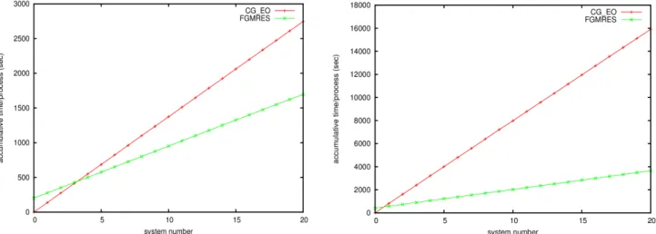
Table 2: Test results comparing timing of FGMRES to CG_EO on ETMC configurations In Table 2, the subspace generation time is the time needed to prepare the deflation subspace. This cost is part of the total FGMRES time and doesn't apply to CG_EO. However, this is a one time cost. In typical lattice computations, tens of right-hand sides is being solved. It means that, this extra setup cost will be quickly compensated by the speedup we get solving the systems using FGMRES. More testing can be done to study the volume and quark mass dependence of the FGMRES solver but these initial results are encouraging. As an illustration of this point, we do another test in which we solve 20 systems. This time we use “Volume” sources and set the solver precision to 1e-16. We also perform the test where block size is 6x6x6x6 since this seems to provide the best performance. In Figure [2] we

(5)

plot the total solver time at the end of each solve for CG_EO as well as FGMRES. Note that the total solve time for system number “0” is the cost of generating the deflation subspace for the case of FGMRES. As can be seen, in both cases the initial setup time gets compensated by the gain in solving the remaining systems. For the B85.24, the overall gain after solving 20 systems is about a factor of 2 while on the larger lattice D15.84 the gain is about a factor of 4. A comment about the number of cores used in these tests is that they are smaller than what would be used in an exa-scale regime. However, the size of the lattice in the case of D15.48 is the largest lattice available at the moment. In addition, the code is designed to require even number of blocks in each direction for each MPI

process. This limited the maximum number of cores that could be used in these tests to 512 cores. It is expected that there will be much larger lattices in the future where the benefit of using less

communications in the case of the AMG solver because of the use of SAP preconditioner will become more apparent.

Figure 2: Accumulative timing for solving 20 systems for the B85.24 case (left) and the D15.48 case (right)

5.2 tmLQCD on Xeon Phi

Our tests on the Xeon Phi have been performed on the cluster at CSC in Finland [4]. TmLQCD is compiled in a native mode using the configure command

./configure --enable-mpi --enable-omp --enable-alignment=64 --enable-gaugecopy --enable-halfspinor --with-mpidimension=4 --with-lapack CC=”mpiicc -mkl -mmic” F77=”ifort -mkl -mmic” CFLAGS=”-std=c99”

As a first test we tried to run the inverter on the B85.24 ensemble on a single MIC card natively using the same parameters as described before. However, this turned out to take a large amount of memory and the code crashed after performing part of the computation. This highlights the anticipated difficulty of limited memory to run the entire code on the MIC. A redesign of the solver will be necessary to take place if one attempts to use the MIC. Alternatively more MIC cards should be used to overcome this problem . Since we had only limited number of MIC cards available we had to use smaller lattice of size L/a=16, T/a=32 hoping that it will fit in memory. The run is done using openMP with 54 threads. In this case the solver has finished and there was no memory problem.

5.3 Performance of the vectorized matrix-vector multiplication

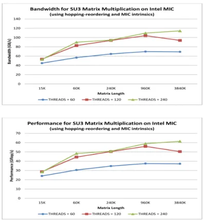
Vectorization of the operations involved in the Lattice Dirac operator is important as described earlier. In Figure [4] we show results that shows the performance of an implementation of the matrix-vector multiplications. These results were obtained by packing the matrices on for lattice sites together as well as the corresponding vectors. The multiplications are then done simultaneously. The results are encouraging, although they are lower than what we would hope for given the peak performance of about 1 Tflops/s that the MIC can provide.

6. Conclusions

(6)

lattice QCD calculations. The solver is tested on multicore machines and found to provide a considerable speedup over the standard CG algorithm. Initial testing of tmLQCD on the Xeon Phi was done and showed the effect of memory limitations requiring further investigation. Work is done towards vectorization of the Dirac operator on the Xeon Phi to benefit from the 512-bit registers available. Two options based on packing the matrices on 4 or 8 lattice sites is given as an approach to achieve this vectorization. Initial performance results for the main operation of multiplying 3x3 matrices times a vector is shown. Although results are encouraging, they are still lower than what is hoped for, requiring further optimizations. In all cases, porting the codes to run on the Xeon Phi was straightforward. Other than the work needed for vectorization, the original code with MPI and openMP could be compiled and run directly on the MIC with no modifications which is a great advantage. These codes are based on tmLQCD and a first version of these codes is available on github as a branch of tmLQCD. After more testing and optimizations, it will be merged to the main branch of tmLQCD which is publicly available. This solver is expected to be beneficial for the current and future simulations done at physical quark masses, large volumes, and small lattice spacing. It will also play an important role on future exascale machines.

Figure 3: performance of the vectorized matrix-vector multiplications on a single MIC card.

References

[1] Andreas Frommer, et. al., “Adaptive aggregation based domain decomposition multigrid for the lattice Wilson Dirac operator”, arXiv:1303.1377[hep-lat].

[2] K. Jansen and C. Urbach, “tmLQCD: A Program suite to simulate Wilson Twisted mass Lattice QCD”, Comput. Phys. Cooun. 180(2009)2717-2738 (arXiv:0905.3331).

[3] https://github.com/etmc/tmLQCD.

(7)

Acknowledgements

This work was financially supported by the PRACE project funded in part by the EUs 7th Framework Programme (FP7/2007-2013) under grant agreement no. RI-312763.

Appendix A: Sample code for vectorization of matrix-vector multiplication in the Dirac operator

In this appendix we list a header file used to perform matrix-vector multiplications for a packed 8 complex 3x3 matrices split into real and imaginary parts.

/**

* Returns the real part of the FMA operation: c = c + a*b * */

static inline __m512d complex_fma_real_512(__m512d c_re, __m512d c_im, __m512d a_re, __m512d a_im, __m512d b_re, __m512d b_im){

c_re = _mm512_fmsub_pd(a_im, b_im, c_re); c_re = _mm512_fmsub_pd(a_re, b_re, c_re); return c_re;}

/*

*Returns the imaginary part of the FMA operation: c = c + a*b */

static inline __m512d complex_fma_imag_512(__m512d c_re, __m512d c_im, __m512d a_re, __m512d a_im, __m512d b_re, __m512d b_im){

c_im = _mm512_fmadd_pd(a_im, b_re, c_im); c_im = _mm512_fmadd_pd(a_re, b_im, c_im); return c_im;}

/**

* Performs the multiplication: chi(3x1) = U(3x3) * psi(3x1) * Each vector or matrix element (e.g. chi[0] or U[1][2]) * is actually a set of 8 complex numbers upon which * operations are performed simultaneously.

* Each complex number is stored in split layout, meaning that * its real and imaginary parts are stored in different vector

* registers. So, the 8 complex numbers contained in chi[0] will actually be * distributed in chi_re[0] and chi_im[0] in split layout.

*/

static inline void su3_multiply_splitlayout_512( __m512d chi_re[3],

__m512d chi_im[3], __m512d U_re[3][3], __m512d U_im[3][3], __m512d psi_re[3], __m512d psi_im[3], __m512d zero){ chi_re[0] = chi_re[1] = chi_re[2] = chi_im[0] = chi_im[1] = chi_im[2] = zero;

chi_re[0] = complex_fma_real_512(chi_re[0], chi_im[0], U_re[0][0], U_im[0][0], psi_re[0], psi_im[0]);// x0 = x0 + U00*y0

chi_im[0] = complex_fma_imag_512(chi_re[0], chi_im[0], U_re[0][0], U_im[0][0], psi_re[0], psi_im[0]);

chi_re[2] = complex_fma_real_512(chi_re[2], chi_im[2], U_re[2][1], U_im[2][1], psi_re[1], psi_im[1]);// x2 = x2 + U21*y

chi_im[2] = complex_fma_imag_512(chi_re[2], chi_im[2], U_re[2][2], U_im[2][2], psi_re[2], psi_im[2]); }