Hamby, Stephen Edward (2010) Data mining techniques
for protein sequence analysis. PhD thesis, University of
Nottingham.
Access from the University of Nottingham repository:
http://eprints.nottingham.ac.uk/11498/1/SEHThesis_Corrected_003.pdf Copyright and reuse:
The Nottingham ePrints service makes this work by researchers of the University of Nottingham available open access under the following conditions.
· Copyright and all moral rights to the version of the paper presented here belong to the individual author(s) and/or other copyright owners.
· To the extent reasonable and practicable the material made available in Nottingham ePrints has been checked for eligibility before being made available.
· Copies of full items can be used for personal research or study, educational, or not-for-profit purposes without prior permission or charge provided that the authors, title and full bibliographic details are credited, a hyperlink and/or URL is given for the original metadata page and the content is not changed in any way.
· Quotations or similar reproductions must be sufficiently acknowledged. Please see our full end user licence at:
http://eprints.nottingham.ac.uk/end_user_agreement.pdf
A note on versions:
The version presented here may differ from the published version or from the version of record. If you wish to cite this item you are advised to consult the publisher’s version. Please see the repository url above for details on accessing the published version and note that access may require a subscription.
Data Mining Techniques for Protein Sequence
Analysis
Stephen Edward Hamby
Thesis submitted to the University of Nottingham
for the degree of Doctor of Philosophy
Abstract
This thesis concerns two areas of bioinformatics related by their role in protein structure and function: protein structure prediction and post translational modification of proteins. The dihedral angles Ψ and Φ are predicted using support vector regression. For the prediction of Ψ dihedral angles the addition of structural information is examined and the normalisation of Ψ and Φ dihedral angles is examined. An application of the dihedral angles is investigated. The relationship between dihedral angles and three bond J couplings determined from NMR experiments is described by the Karplus equation. We investigate the determination of the correct solution of the Karplus equation using predicted Φ dihedral angles. Glycosylation is an important post translational modification of proteins involved in many different facets of biology. The work here investigates the prediction of N-linked and O-N-linked glycosylation sites using the random forest machine learning algorithm and pairwise patterns in the data. This methodology produces more accurate results when compared to state of the art prediction methods. The black box nature of random forest is addressed by using the trepan algorithm to generate a decision tree with comprehensible rules that represents the decision making process of random forest. The prediction of our program GPP does not distinguish between glycans at a given glycosylation site. We use farthest first clustering, with the idea of classifying each glycosylation site by the sugar linking the glycan to protein. This thesis demonstrates the prediction of protein backbone torsion angles and improves the current state of the art for the prediction of glycosylation sites. It also investigates potential applications and the interpretation of these methods.
Acknowledgements
I thank Jonathan Hirst for his excellent supervision, Ben Bulheller for designing the website that makes the glycosylation prediction software available for use, Clare Evans, Craig Bruce, and Petros Kountouris for useful discussions, the BBSRC for a studentship and the University of Nottingham for the use of high performance computing.
Contents
Abstract iii
Acknowledgements iv
List of Figures x
List of Tables xii
List of Common Abbreviations xiii
Publications Arising From This Thesis xv
Chapter 1 Protein bioinformatics 1
1.1 Introduction 1
1.2 Sequence analysis 3
1.2.1 PSI-BLAST 4
1.3 Protein structure 6
1.3.1 Dihedral angles 10
1.3.2 Secondary structure prediction 12 1.3.3 Prediction of dihedral angles 16 1.3.4 Hydrophobicity and surface accessibility 18 1.3.4.1 Assignment of hydrophobicity and surface accessibility 18 1.3.4.2 Prediction of solvent accessibility 19
1.4 Post translational modification 21
1.4.1 Post translational modification overview 22
1.4.2 Glycosylation 23
1.4.3 Structure of glycans 24
1.4.3.1 Carbohydrates 24
1.4.3.2 Monosaccharides 24
1.4.3.4 Oligosaccharides 25
1.4.4 Glycosyltransferases 26
1.4.5 N-Linked glycosylation 27
1.4.5.1 Function of N-glycans 29
1.4.6 O-Linked glycosylation 30
1.4.6.1 O-GalNAc or mucin type modification 30 1.4.6.2 Functions of O-linked mucin glycans 32 1.4.7 Glycosylation of cytosolic and nuclear proteins 33
1.4.8 Prediction of glycosylation 34
1.4.8.1 Previous prediction methods 35
1.4.8.2 Motivation and objectives for new predictive methods 36
1.5 Thesis overview 36
1.6 References 37
Chapter 2 Machine learning algorithms 46
2.1 Introduction 46
2.2 Classification 48
2.3 Decision trees 50
2.3.1 Decision tree induction 51 2.3.2 Splitting criteria 51 2.3.2.1 Impurity based criteria 51
2.3.2.2 Binary criteria 54
2.3.3 Stopping criteria and pruning 54 2.3.4 Some decision tree algorithms 56
2.4.1 Decision forest: general principles 57
2.4.2 Diversity 59
2.4.3 The combiner 62
2.4.4 Random forest 63
2.5 Kernel based machine learning 65
2.5.1 Kernel types 66
2.5.2 Hard margin support vector machine 68
2.5.3 Soft margin classifier 68
2.5.4 SVR 68 2.6 Critical assesment 69 2.6.1 Assessing accuracy 70 2.6.2 Model interpretability 72 2.6.2.1 Neural networks 73 2.6.2.2 SVM 76 2.6.2.3 Random forest 78 2.7 References 79
Chapter 3 Dihedral angle prediction 85
3.1 Introduction 85
3.2 Methods 87
3.2.1 Datasets 87
3.2.2 Data pre-processing and representation 88
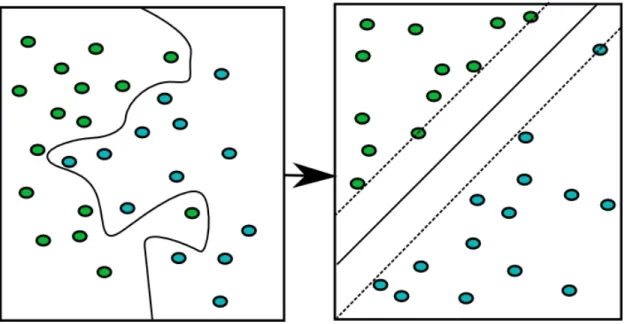
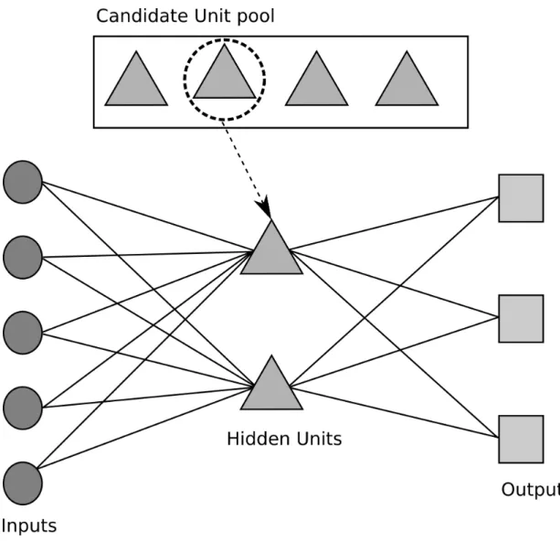
3.2.3 Structure prediction with cascor 90
3.2.4 Dihedral prediction with SVR 93
3.2.6 Optimisation 96 3.2.7 Training and evaluation for dihedral angle prediction 98
3.2.8 Normalisation 100
3.3 Results and discussions 100
3.3.1 Initial predictions 100
3.3.2 Effect of normalisation 103 3.3.3 Effect of addition of amino acid properties 104 3.3.4 Predicting Φ angles 105 3.3.5 Applications of predicted dihedral angles to assigning 106 NMR spectra
3.3.6 Predicting the correct solution for BioMagRes 106 J coupling data
3.4 Conclusions 109
3.5 References 110
Chapter 4 Glycosylation prediction 114
4.1 Background 114
4.2 Methods 118
4.2.1 The dataset 118
4.2.2 Frequency analysis 119 4.2.3 Balancing the dataset 122
4.2.4 Training the prediction program 125
4.2.5 Extraction of rules 129
4.3 Results and Discussion 130
4.3.2 Pairwise patterns 133 4.3.3 Prediction accuracy 136 4.3.4 Rule extraction 140 4.3.5 Sugar type 143 4.4 Conclusions 147 4.5 References 148 Chapter 5 Conclusions 153 5.1 References 158 Appendix A 159 Appendix B 163 Appendix C 165 Appendix D 169
List of Figures
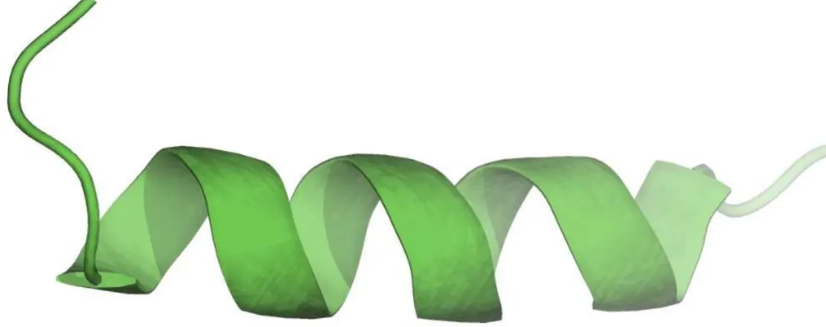
1.1 An example of an α helix structure from the UBA domain of the 7 protein p62
1.2 The hydrogen bonding pattern of an anti-parallel β sheet 9 1.3 Dihedral torsion angles of the protein backbone 10
1.4 The Ramachandran plot 11
1.5 Glycosyltransferase A 26
1.6 The synthesis and maturation of N-glycans 28
1.7 Four common O-glycan core structures 31
2.1 A general schematic of a simple decision tree 50 2.2 An illustration of kernel machine learning where a maximal margin 66
hyperplane can be fitted to the data on the left after it has been raised into a higher dimensional space by a kernel function from its
representation on the right
3.1 Schematic of the cascade correlation network 92
3.2 An example of an input vector for CASCOR 92
3.3 An example input vector for dihedral angle prediction 96 3.4 Example input for prediction of dihedral angles with the addition 99
of secondary structure
3.5 An example of the input including amino acid parameters 104 4.1 The flow of data through the prediction program 120 4.2 The cross-validation of the GPP prediction program, illustrated for 127
the Ser dataset
4.3 Asn glycosylation rules 141
4.5 Ser glycosylation rules 143 C.1 Complete decision tree for Asn glycosylation 166 C.2 Complete decision tree for Ser glycosylation 167 C.3 Complete decision tree for Thr glycosylation 168
List of Tables
3.1 Correlation coefficients achieved using various SVR kernel functions 101 3.2 Initial results of SVR prediction with and without optimisation and 102
in comparison to previous work
4.1 Frequencies of selected amino acids surrounding modified Asn 131 residues
4.2 Frequencies of selected amino acids surrounding modified Ser 132 residues
4.3 Frequencies of selected amino acids surrounding modified Thr 133 residues
4.4 The 20 most significant patterns for glycosylated residues 134 4.5 Accuracy of prediction of glycosylation sites with random forest 137
and na•ve Bayes algorithm
4.6 A comparison of the GPP predictor and other glycosylation 138 prediction programs
4.7 Percentage membership of clusters generated by farthest first 145 clustering of Ser glycosylation sites
4.8 Percentage membership of clusters generated by farthest first 146 clustering of Thr glycosylation sites
B.1 Frequency statistics for glycosylated Asn residues 163 B.2 Frequency statistics for glycosylated Ser residues 164 B.3 Frequency statistics for glycosylated Thr residues 164
List of Common abbreviations
For abbreviations of amino acid names and sugars refer to appendices A and D respectively.
ASA Accessible Surface Area ATP Adenosine Tri Phosphate
BLAST Basic Local Alignment Search Tool
BLOSUM BLOcks of Amino Acid SUbstitution Matrix CART Classification and Regression Trees
CASCOR CAScade CORrelation
CASP Critical Assessment of methods for protein Structure Prediction CCI Correctly Classified Instances
Da Dalton
DESTRUCT Dihedral-Enhanced STRUCTure prediction DNA Deoxyribose Nucleic Acid
DSSP Define Secondary Structure of Proteins ER Endoplasmic Reticulum
GPI Glycophosphatidylinositol HMM Hidden Markov Model kDa kilo Dalton
MAE Mean Absolute Error
MCC Matthews Correlation Coefficient NMR Nuclear Magnetic Resonance PAM Percent Accepted Mutation PCC Pearson Correlation Coefficient PDB Protein Data Bank
PSI-BLAST Position Specific Iterated BLAST PSSM Position Specific Scoring Matrix PTM Post Translational Modification RMSE Root Mean Squared Error RNA Ribose Nucleic Acid
RSA Relative Solvent Accessibility SA Solvent Accessibility
SNP Single Nucleotide Polymorphism SVM Support Vector Machine
Publications Arising From This Thesis
Hamby SE, Hirst JD, Prediction of glycosylation sites using random forests. BMC Bioinformatics 2008, 9:500.
Chapter 1: Protein Bioinformatics
1.1 Introduction
Proteins are the work horses of biology. Both within the cell and without and across the whole spectrum of life there are proteins. They fulfil a structural role, such as in the case of collagen, which provides the framework of connective tissue, and they are the machines of biology, catalysing the chemical reactions of life throughout the biosphere. Protein biology has long been studied by scientists interested in a wide range of organisms. Proteins are important for the understanding of biology in healthy and disease states as well as providing drug targets against pathogenic organisms, and they are even potentially drugs themselves.
The function of a protein depends on its structure. Therefore, much effort has been devoted to the determination of protein structures. Experimentally, a wide range of techniques have been used to study protein structure and dynamics. X-ray crystallography and NMR have been used to determine protein structure, and NMR spectroscopy has also been used to study protein dynamics. These methods are expensive and time consuming. Some structures, particularly membrane proteins, are very difficult or impossible to characterise experimentally. A computational approach can, therefore, be advantageous. Bioinformatics methods aim to predict the structure of proteins using the amino acid sequence and properties of the amino acids that are readily available. Rather than predict the 3D structure of the entire protein, which is very difficult, due to the number of possible structures that a given sequence can adopt, the problem is often broken down into smaller tasks, such as the prediction of secondary structure or of dihedral angles. Much work has been done on the prediction
Post translational modification (PTM) of proteins is heavily involved with the regulation of proteins and with structural and functional aspects of proteins. Glycosylation, which we focus on in the second part of this thesis, is involved in a wide number of biological processes. Therefore, it is important to be able to determine where a protein is glycosylated and precisely which carbohydrate is joined. Once again determination of this is expensive and time consuming. This has led to a computational approach being employed to determine the location of the glycosylation sites (and indeed other PTMs).
The bioinformatics problems dealt with in this thesis are sequence analysis problems. For this reason, we begin by introducing sequence analysis and reviewing the methods used to compare biological sequences, which are essential to the field. In the first part of this chapter, we review methods for predicting secondary structure, dihedral angles and surface accessibility of proteins. In chapter 3, we present our research on the prediction of dihedral angles of proteins and its potential applications.
The second part of this introduction gives some background on PTM of proteins. A major aspect of protein structure and function, PTMs are structural modifications to a protein where a small molecule is added to a specific amino acid. These modifications are important in many areas of biology, such as the regulation of proteins and DNA, and signalling between cells and molecules. We give an overview of the different types of PTM and introduce glycosylation, a PTM where carbohydrate is added. In chapter 4, we describe our work to predict glycosylation sites and use the model generated to find out information about what determines the location of a
glycosylation site.
1.2 Sequence Analysis
In biology, there are two main areas of sequence analysis: sequence comparison, i.e., multiple sequence alignment, and prediction using sequence analysis, although the first is often used as a starting point for the second. Multiple sequence alignment is the comparison of three or more sequences.1 It is often used to find homologous sequences in a large database and to align known homologues. This process of locating and aligning homologous sequences is central to bioinformatics and is the most important area of sequence analysis. Initially, dynamic programming algorithms were prohibitively slow, with both stochastic and tree-based methods being attempted. The introduction of progressive alignment methods in the 1980s has been the foundation for modern sequence alignment methods, a selection of which are reviewed below. Progressive alignment allows a full alignment to be built up gradually, using a tree as a guide for the alignment. It forms the basis of some of the most popular sequence alignment programs, such as clustalW.2 ClustalW creates a distance matrix using dynamic programming combined with a sequence weight matrix, such as PAM3 or BLOSUM.4 The neighbourhood joining method produces a guide tree for progressive alignment based on this matrix. The progressive alignment is carried out by conducting the pairwise alignment of sequences using the tree as a guide, thus aligning more and more sequences with each iteration, until the alignment is completed. Version 2.0 of this program5 allows faster and more accurate alignments.
sequence alignment programs to improve the accuracy of alignments by including evolutionary information. The level of pairwise similarity between two given amino acids can be measured by the likelihood of an amino acid substitution occurring by chance versus being inherited. This can be quantified by the number of point mutations required to go from one amino acid to the other. This is known as the evolutionary distance between two amino acids. Dayhoff et al. used this principle to develop a series of mutation matrices3. These PAM matrices are derived from the assumption that evolution proceeds by way of single point mutations. Mutation matrices can be used to find the optimal sequence alignment, the one most likely to have occurred by evolution from a common ancestor rather than by chance.
The BLOSUM matrix is calculated in a similar way to the Dayhoff matrix. Henikoff and Henikoff use sequence blocks taken from regions highly conserved between sequence families4. The sum of pairwise sequences for these blocks is used to calculate an odds matrix in similar fashion to the Dayhoff matrix. Sequences are clustered based on percentage identity, in order to allow differing evolutionary distances to be included. This results in a series of matrices equivalent to the PAM matrices developed by Dayhoff. BLOSUM62 is the most commonly used, the 62 indicating it was compiled using clustering at 62% identity.
1.2.1 PSI-BLAST
One of the programs that has most revolutionised bioinformatics is PSI-BLAST (position specific iterated BLAST). 6 PSI-BLAST identifies homologous sequences from a database using BLOSUM62 matrices. It is also used to generate position specific scoring matrices (PSSMs). PSI-BLAST profiles are used in a number of
sequence alignment methods and in many other areas of sequence analysis as a way of representing the amino acid sequence. The generation of these profiles is discussed in chapter 4. PSI-BLAST is an enhancement of the BLAST algorithm,7 used for searching protein and DNA databases for homologous sequences. BLAST uses well- defined sequence similarity measures in the form of PAM matrices to approximate the results that would be obtained using dynamic programming methods. PSI-BLAST improves over BLAST in both computation time and accuracy, by using sequence profiles to perform an iterative search of the database. PSI-BLAST allows for the generation of gapped alignments, reducing the number of potential alignments that need to be searched for the optimal alignment. PSI-BLAST also automatically generates a PSSM from the significant alignments found in a given iteration and uses this as input for the next iteration. Profile based searches are more sensitive to distant homologies than pairwise based alignments. A PSSM represents the similarity and evolutionary distance for each amino acid in a protein relative to all of the 20 standard amino acids (see chapter 3 for a more detailed description and an example). The PSSM profiles are often used as input to other methods, e.g., as the input to a prediction program, since they represent an amino acid sequence in a way, which includes evolutionary information. The level of conservation of a group of amino acids is important when relating sequence to function. In this work, we use PSSMs as an input for prediction of both secondary structure and real value dihedral angles (Chapter 3). We use PSI-BLAST with multiple iterations to generate these, because of the ease of obtaining PSSMs from PSI-BLAST and because of the track record of the program being used in a similar manner. Other methods described are described briefly below.
There have been many attempts to enhance the PSI-BLAST algorithm and many sequence alignment programs use PSI-BLAST profiles to enhance alignments. HHPred8 combines PSI-BLAST with hidden markov models (HMMs). Rangwala and Karypis9 use PSI-BLAST as the base for an incremental alignment method based on sequence windows. CTX-BLAST10 incorporates a contextual alignment model into PSI-BLAST. Lee et al.11 tackle the problem of an increased probability of the introduction of false positives with each subsequent iteration of PSI-BLAST by introducing a ranking of hits produced from the first and last iteration. Przybylski and Rost12 boost the performance of PSI-BLAST using consensus sequences. We prefer the standard version of PSI-BLAST over these, as none of these readily outputs a PSSM without alteration, and not all are easily available.
1.3 Protein Structure
Sequence analysis has been used for the prediction of many different biological properties. It is common to use PSI-BLAST profiles to represent the protein sequence for prediction experiments. The goal is to determine some property of the protein from its amino acid sequence. Some of the most researched areas are structure prediction, both tertiary and secondary.
Anfinsen showed that all of the information about a protein can be determined from its primary structure.13 The primary structure of a protein is the sequence of amino acids from N terminus to C terminus. The structures of the 20 amino acid types are given in Appendix A. There has been evidence for the contribution of environmental factors to protein folding and structure, and PTMs also play a role in determining the final structure of a protein. However, it is likely that a reasonable approximation of the 3D
structure of a protein in its native state can be determined from the primary structure with no additional information. This is, however, a calculation with too many permutations to be achieved ab initio. As a result of this, many less complex problems have been defined, to provide a bridge to predicting the complete structure. These include prediction of secondary structure, of dihedral angles, the prediction of surface accessibility of amino acid residues and prediction of residue contacts.
A stepping-stone to the 3D structure is the secondary structure. This consists of a series of structural motifs that occur often within proteins. These can be considered as building blocks, which form the bulk of the proteinÕs structure. The secondary structure is most comprehensively described using the eight states assigned by the program DSSP14, although this is often reduced to a three state description of secondary structure. DSSP assigns structure based mainly on the hydrogen bonding patterns of a protein. These are used to assign the states of α-helix and 310-helix, β -sheet, β-bridges, π-helices, turns and bends.
An α helix (figure 1.1) is a regular helical arrangement of the amino acids held in place by the formation of amide to carbonyl hydrogen bonds. There are 3.6 residues per turn, with a rise between residues of 1.5 •. Such helical structures can range in length from four amino acids to 40 or more and are sometimes amphipathic in nature. The helical structure can be broken (or prevented) by the inclusion of Pro, Gly, Ser or Thr in the sequence. Residues that encourage helix formation are Ala, Glu, Leu and Met.
310-helices consist of three residues per turn and each hydrogen bond encloses a ring of ten atoms. Main chain hydrogen bonds are separated by three residues. Often occurring at the end of α-helices, 310-helices are less stable than α-helices, because the dipoles are less well aligned. This also means the packing is less energetically stable than that of an α-helix. In a π-helix, the hydrogen bonds are formed between residue i and residue i+5. This secondary structure element is a rare occurrence and long π-helices are not found.
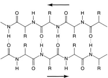
β-sheet (figure 1.2) takes the form of a planar arrangement of the amino acids, where the amino acids line up in extended conformation in stretches of five to ten residues. Typically the surface of this is corrugated in shape. β-sheets can be either parallel or anti-parallel in form. In parallel β-sheets the direction of the amino acid chains within the sheet is the same throughout. These tend to have a longer distance in the sequence between the strands in the sheet, with long loop structures and random coil sections filling the gaps. Alternating direction of the amino acid backbone characterises anti-parallel β-sheets. This form of β-sheet is often linked by short loops such as β-turns. An isolated pair of parallel β-sheet type structures is known as a β-bridge.
The loops and turns in a protein structure can take several forms. Turns are usually three to ten amino acids in length, and have defined structure, whereas loops are generally disordered in structure (i.e., random coil) and can be any length. Loop regions, in particular, are often of functional importance and can change conformation in order to facilitate binding of molecules. β-turns may be as few as three residues long and consist of a single hydrogen bond between two residues, which bends the amino acid sequence into a hairpin shape. There are several variations on the basic β -turn and this type of structure may also be known as a bend or hairpin. Anything not conforming to the above structural motifs is classified as random coil. Such structures form a large proportion of protein structures.
Figure 1.2. The hydrogen bonding pattern of an anti-parallel β-sheet. Dashed lines are hydrogen bonds and the arrows indicate the direction of the chain. (Image released under the creative commons licence.)
The supra-secondary structure of a protein is a further progression towards the 3D structure. Certain commonly identified structural motifs that are made up of secondary structure elements, such as those described above, can be the first to form when a
protein folds into its native structure. These include structures such as the β-barrel or the α-helical bundle, as well as structural motifs involving loops and both β-sheets or
α-helices. Many such supra-secondary structure motifs have been described.
The tertiary structure of a protein is its complete 3D structure. This structure is determined by weak interactions between amino acid residues and side chains. Interactions such as steric hindrance, electrostatic, hydrophobicity related interactions, and van der Waals interactions all play a role.
1.3.1 Dihedral angles
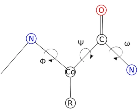
Figure 1.3. Dihedral torsion angles of the protein backbone. The location of the backbone dihedral torsion angles Φ, Ψ, and ω are shown by the dashed lines indicating rotation around a bond.
Dihedral torsion angles are described by rotation around the bonds along the protein backbone (figure 1.3). Of the three backbone dihedral angles, ω is generally planar, i.e., 0¡ in the cis conformation and 180¡ in the trans conformation. This is due to the
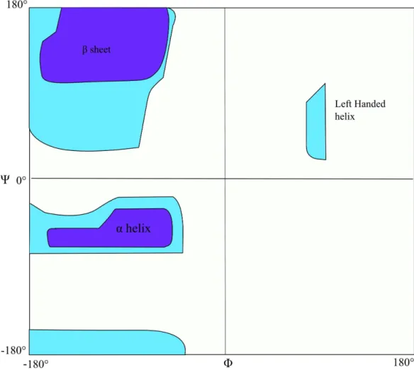
delocalisation of the carbonyl π electrons and the lone pair of the nitrogen atom. The other backbone dihedral angles are limited by steric hindrance. In practice, only 10% of the available conformations of Ψ and Φ angles are observed. Ramachandran15 examined the available conformations in a selection of proteins, treating each atom as a hard sphere based on its van der Waals radius and disallowing steric clashes.
Figure 1.4. The Ramachandran plot. The regions are labelled with the type of secondary structure indicated by the angles found there. The light shaded areas encompass allowed angles including those of glycine. The dark shaded areas show angles not including glycine.
similar values of Φ and Ψ for a given structure type. From the dihedral angles it is possible to get an approximation of the structure of a protein. Thus, it is useful to have a prediction of the dihedral angles for tasks such as structure prediction (both secondary and tertiary). There have been many attempts to predict the secondary structure of a protein and, more recently, several attempts have been made to predict
Ψ and Φ dihedral angles.
1.3.2 Secondary Structure Prediction
Elements of secondary structure were first proposed by Pauling16.Attempts to predict the location of the secondary structure elements have been ongoing ever since, using a variety of methodologies. These are too numerous for all of them to be described here. However, the most important are presented below with some historical perspective. We use secondary structure prediction in both the areas of research covered in this thesis. It is a major component of our work to predict dihedral angles as we hypothesise that using secondary structure prediction will improve the accuracy of dihedral angle prediction, and in chapter 4 we use secondary structure prediction to add extra information to the input for our glycosylation predictor.
Initial attempts at secondary structure prediction centred around amino acid propensity. GOR17, now at version V18, in its first version only used single residue statistics within a sliding sequence window. The statistics are generated for residues within the sequence window, with the objective of predicting the state of the residue at the centre of the window. By sliding the window along the length of the sequence, it is possible to obtain predictions for the entire protein. Subsequent versions of the program improved by adding pairwise statistics (version II18) and information
theoretic methods (version III and IV18). In version V, the information theory methods previously employed are combined with evolutionary information via PSSMs obtained from PSI-BLAST. The GOR algorithm uses a combination of information theory and Bayesian statistics to predict secondary structure. When combined with PSI-BLAST, this produces an accuracy of 73.5% Q3, although this has since been improved upon. Q3 is the three state prediction accuracy for protein secondary structure (equation 1.1)
Q3= p
( )
α + p( )
β + p coil(
)
N (1.1)
where p is the number of residues correctly predicted for a given secondary structure type and N is the total number of residues.
PHD19 is a neural network based prediction method, consisting of a three level feed forward network. The first level of the network takes as input a multiple sequence alignment and assigns the central residue of a 20 amino acid sliding window to one of the standard three structural classes. The second level takes the output of the first as input and once again predicts the structure class. The input from the preceding network is expressed as a 17 amino acid window, with amino acids represented by three binary outputs describing the structure classification. A number of such networks were trained and the outputs were fed into the third level of the network. The third level represents a jury decision by arithmetic average that produces a final prediction for secondary structure class. This schema produces accuracy of 70% (Q3).
Another neural network based method, and one of the most popular secondary 20
This method uses PSSMs generated by PSI-BLAST as input for a neural network. This was the first method to use such profiles directly rather than compiling a complete multiple sequence alignment. The output of the initial feed forward neural network is then filtered by a second network to give the secondary structure prediction. This gives an accuracy of around 76%. Here we use predictions from PSIPRED as input for glycosylation prediction in the hope of improving accuracy (see chapter 4).
HMMSTR21 uses HMMs for secondary structure prediction as well as other protein properties. The model is based on sequence structure motifs and uses a voting scheme to determine the final structure. The HMMs used are different in that they are not the typical profile HMMs used in many other models. The model uses the correlations between sequence structure motifs to reduce the number of parameters in the model, and predicts secondary structure with an accuracy of 74.3% (Q3).
JNET22 uses a neural networks arrangement which is similar to that used by PHD, using PSSMs produced by PSI-BLAST as input. JNET predicts secondary structure with an accuracy of 76.4% (Q3). A different approach is taken by Pollastri et al.23 Their program SSPro uses a bidirectional recurrent neural network for secondary structure prediction with PSSMs. The performance of SSPro is 77%-80% (Q3), dependent on the testing set used. A brute force local clustering method is proposed by Jiang.24 This tries to take into account long range interactions, which form a significant component of protein structure.25
structure and dihedral angles. Initially, two neural networks are trained, one predicting secondary structure and one predicting the Ψ dihedral torsion angle. The output from each is fed into subsequent neural networks in an iterative manner; the predictions of
Ψ are used to enhance predictions of secondary structure and visa versa. The resulting prediction of secondary structure is comparable in accuracy to PSIPRED. This prediction program will be discussed in some detail later, as it forms a basis for some of the work in this thesis.
Montgomerie et al. developed the program proteus.27 This includes structural alignments as part of the prediction process, and achieves a Q3 score of 88% by combining the secondary structure predictors of PSIPRED, JNET and TRANSSEC27 (TRANSSEC was developed by the authors) as a ÒJury of expertsÓ. Birzele and Kramer28 define a new representation of secondary structure based on frequently occurring patterns. The authors use this to perform a prediction with a Support Vector Machine (SVM) classifier, which is comparable to PSIPRED in accuracy. A more traditional approach to prediction using SVMs is taken by Karypis.29 Using a novel kernel function cascaded SVMs are trained to predict three state secondary structure with of 79.3%. SVM classification is an opaque method. He et al.30 use an SVM in combination with a decision tree to extract meaningful rules with regard to protein secondary structure. The SVMs average 77.6% accuracy for helix, 80.7% for sheet and 70% for coil. Zhong and co-authors31 use k-means clustering to divide the training sets into representative clusters. This allows them to use their method of clustering SVMs to make predictions of secondary structure, which are in the region of 80%, although this varies across the clusters obtained. Won et al.32 use genetic algorithms to evolve a HMM for secondary structure prediction. The model developed improves
over HMMSTR, but is still much less accurate than state of the art models for secondary structure prediction. Prof33 is an ensemble method consisting of multiple neural networks combined using simple linear discrimination and a further neural network. The neural networks used are based on the methods GOR and PSIPRED. The combined result gives an accuracy of 77% (Q3). Yao et al.34 predict secondary structure using a probabilistic model. The authors combine the dynamic Bayesian method with a neural network. This combination gives results that are comparable with state of the art methods.
1.3.3 Prediction of dihedral angles
The Ramachandran plot clearly shows the link between the dihedral angles and protein structure. Thus, it is useful to predict dihedral angles. The DESTRUCT method26 uses dihedral angles to improve the accuracy of secondary structure and predictions of secondary structure to improve the accuracy of dihedral angle predictions. DESTRUCT was the first server to predict real value dihedral angles, achieving a Pearson correlation coefficient (PCC, see chapter 2 for definition) of 0.47. Previously, HMMSTR21 predicted categories for dihedral angles, using HMMs in a manner similar to the method for predicting secondary structure described above. A more recent method for predicting dihedral angle regions is DHPred.35 The authors define dihedral angle regions H, E and O (outlier) based on the Ramachandran plot. Residues are classified as belonging to a particular dihedral angle region using SVMs. The authors employ a two level approach to classification. First, sequences represented by PSSMs generated by PSI-BLAST are input into the first SVM classifier, which outputs predictions for each of the three dihedral angle regions considered. Secondly, these predictions are combined with the PSSM with a sequence
window size of seven and used as input for the second SVM classifier, which produces the final predictions for the state of each residue. This results in an accuracy of approximately 80%, comparable to the accuracy of PSIPRED and other secondary predictors, a legitimate comparison given that the dihedral regions correspond to the three state secondary structure of proteins. DESTRUCT was primarily motivated towards secondary structure prediction, with the dihedral prediction having the sole purpose of improving secondary structure accuracy. For this reason, only the Ψ
dihedral angles are predicted by DESTRUCT. The other dihedral angles are less significant with regard to the definition of secondary structure, although Φ does play an important role when considering the tertiary structure.
Real Spine36 improves substantially upon DESTRUCT. The first version gives a correlation coefficient of 0.62 between predicted and actual Ψ dihedral angles. The authors use twin neural networks. The inputs to both networks consist of PSSM profiles combined with predicted secondary structure information. The two networks produce a consensus prediction by averaging the output of the networks. Real Spine also predicts relative solvent accessibility (RSA) using the same methodology. The prediction for RSA has a correlation coefficient of 0.74. Real-Spine 2,37 the second version, substantially improves over Real Spine, using a very simple alteration. Due to the properties of the sigmoidal function, the neural networks of Real Spine function poorly with respect to predictions in the region between -36¡ and +36¡. The dihedral angle distribution is shifted by a normalisation step so that there are relatively few angles in this region. This small adjustment improves prediction accuracy to 0.75 (PCC). Unlike its predecessor, Real-Spine 2 does not predict RSA values. However, it is the first to produce real-value predictions for Φ as well as Ψ. The method employed
for predicting Φ is similar to that for Ψ. However, the normalisation used is different to allow for the differing distribution of Φ.
Whilst there are limits to predictive power, it is clear that there is much scope for improvement in the prediction of real value dihedral angles. Such improvement would enable the dihedral angles to be used to accurately predict the 3D structure of proteins, and potentially to aid in the assignment of structure from NMR spectra. In this work we hypothesise that we can improve on the above prediction methods by selecting a new machine learning method and use secondary structure prediction to enhance the accuracy of the prediction method. We selected Support vector regression (SVR) for this purpose. A detailed discussion of the reasoning behind this is presented in chapters two and three. Later, we also apply the normalisation methodology of Real Spine to SVR.
1.3.4 Hydrophobicity and Surface Accessibility
In our work to predict glycosylation sites, we use information about both hydrophobicity and surface accessibility, as these are both key properties. We include them, as PTMs can only take place on the outside of a protein and so finding those residues with high surface accessibility may improve accuracy. Here, we give an overview of these two properties and review methods for surface accessibility prediction.
1.3.4.1 Assignment of Hydrophobicity and Surface Accessibility
Hydrophobicity is a defining property of protein structure. A molecule is hydrophobic if it is repelled by water and hydrophilic if the opposite is true, hydrophobicity is the
degree by which molecules are repelled by water and is a sliding scale. Amino acids can be divided into two groups based on their hydrophobicity i.e. whether they are hydrophobic or polar. Hydrophobic amino acids are more likely to be found in the centre of a globular protein, or in the membrane bound sections of a membrane protein. Polar amino acids are more likely to be found near the surface. There are various hydrophobicity scales,38 which rank the amino acids according to their degree of hydrophobicity. There are, however, instances when buried residues are polar or exposed residues are hydrophobic, usually due to structural considerations or because of the need for functionality.
Another approach is to consider the surface area that is exposed to solvent whilst in a given protein. This is known as the accessible surface area (ASA). The solvent accessibility of a protein is a related quantity, which can be determined by estimating the number of water molecules in contact with the amino acidÕs surface. This value is calculated from molecular coordinates by DSSP, and is known as relative solvent accessibility when expressed on a continuous scale normalised with respect to the maximum solvent accessibility of each residue.39
1.3.4.2 Prediction of Solvent Accessibility
RSA can be predicted as either a real value or projected onto a series of discrete states. Other methods also predict the ASA area directly. The neural network based predictor developed by Rost and Sander39 achieves only modest accuracy for a ten state prediction of RSA. The ten states are selected to give a finer grained distinction of RSA levels near to the protein core. The method then uses an arrangement of neural networks to predict RSA. The arrangement of neural networks is similar to that used
in PHD, described previously.
The majority of methods predict solvent accessibility as a number of categories, although it is ideally preferable to obtain a real value, as RSA is a sliding scale. In our work we use real value predictions. However, we also give a brief overview of some categorical predictors for both historical context and completeness. Li and Pan40 use multiple linear regression to predict two state solvent accessibility. Yuan et al.41 predict two state solvent accessibility using SVM classifiers. Pollastri et al42. use bidirectional recurrent neural networks (RBNN) to predict both solvent accessibility and contact number. Multiple networks are trained and evaluated by cross validation. RVP-NET43 uses neural networks to predict real values for solvent accessibility. This method gives a PCC of 0.45-0.46 depending on the test data used. Kim and Park44 predict relative solvent accessibility as both a two and three state classification, employing various thresholds. SVM predictions are combined by the use of a directed acyclic graph based scheme. The resulting method, PsiSVM, produces an accuracy of 78% for two state prediction. Wang et al.45 use multiple linear regression to predict real values for solvent accessibility. The sequences are represented by PSSMs and prediction is comparable to other methods.
Multiple linear regression is also employed by Qin et al.46 for the prediction of both solvent accessibility and secondary structure. QBES47 presents a substantially different approach to predicting solvent accessibility. The authors use quadratic programming as a means of minimising a simple energy function. Gianese and Pascarella48 employ a consensus method comprising the predictors JPRED, AccPro and PP.49 PP was produced by Gianese et al.49 and uses profiles of conditional
probabilities to perform its task. The three predictors are combined using a state mapping approach to two state RSA prediction to produce the consensus. SVM Cabins50 integrates the two approaches of classification and regression to improve the accuracy of solvent accessibility prediction.
SABLE51 is a method based on neural networks for regression in order to predict real values for RSA. The method is trained on a large non-redundant dataset derived from Pfam52. The sequences are represented using PSSMs extracted from PSI-BLAST. The authors test both feed forward and Elman53 networks for prediction. The final predictor achieves a correlation coefficient of 0.66. We chose to use SABLE in this work for several reasons. Firstly, it is both freely available and open source allowing ease of use and integration with our existing software, whilst being reasonably accurate in predicting real values for solvent accessibility. Although more accurate methods exist, they were not easily available for use.
1.4 Post Translational Modification
Proteins are synthesised in the body by way of transcription and translation, before folding into their final structure. All proteins start out as a DNA sequence. This is transcribed into messenger RNA. In the case of eukaryotic organisms, the sequence undergoes RNA splicing, which can alter the order of exons to produce novel products. Introns are removed during this process. The messenger RNA is transformed into protein sequence by the ribosome, transfer RNA brings the appropriate amino acids to the ribosome and adenosinetriphosphate (ATP) is consumed to bind together the amino acids using the messenger RNA code as a template. The protein folds into its final structure, either in the cytosol or is transferred to the endoplasmic reticulum
(ER). Many proteins require chaperones to fold into the final structure. These chaperone proteins are also involved in a quality control process to ensure correct folding.
After proteins are created in the body they can undergo a variety of modifications essential for the correct folding and functionality of the protein54. There are over a hundred types of PTM, but some of the most common are briefly discussed below. These modifications can be either transient or permanent and often confer function on the protein in question. They occur across the entire spectrum of life. These modifications can be classified by the molecule added during the modification. There are also PTMs involving protein cleavage by proteases. However, it is beyond the scope of this thesis to discuss these here. The most common types of PTM are phosphorylation, acylation, alkylation, glycosylation, and oxidation, although there are many others. In this work we focus on the prediction of glycosylation sites from sequence with some additional work aimed at understanding the models that generate these predictions. Our hypothesis is that even where no consensus sequence motif exists there will be certain amino acids that favour glycosylation. So for this reason we use information on the pairs of amino acids surrounding glycosylation sites with the hypothesis that this will lead to a higher accuracy of glycosylation prediction.
1.4.1 Post Translational Modification Overview
Here we give a brief overview of some common types of PTM before going on to give a more extensive overview of glycosylation. Phosphorylation54,55 occurs upon the addition of a phosphate group to either Ser, Thr or Tyr. This particular modification is important for regulating cell processes and for signalling both within and between
cells. Some phosphorylation sites are transitive yin yang sites. In such cases the site can either be phosphorylated or glycosylated, depending on the physiological conditions and the environment of the protein. Such sites are often important as regulatory elements in the cell cycle and in signalling processes. As such, the functions and regulation of phosphorylation and cytoplasmic O-glycosylation are intricately linked. Acylation encompasses the addition of fatty acid chains of length C2, C14, C16, and the 8kDa chain of ubiquitin. Acetylation56 is the addition of multiple lysine residues to the histone terminus. In myristoylation57 a mirosyl group is added via glycine to the protein and effects the movement of the protein towards membrane interfaces. In palmitoylation58 the acyl group is transferred to the thiolate chain of cystine. This modification is also involved in the membrane anchoring of proteins. Ubiquitylation59 involves the carboxyl terminus of the protein ubiquitin being added to lysine. This is either added as a single molecule (mono-ubiquitylation) or as the stepwise addition of multiple ubiquitin segments. Poly and mono-ubiquitylation both are involved with the direction of proteins to new locations within the cell. Alkylation involves the addition of alkyl substituents of varying size to several different amino acids. N-linked methylation60 of Lys and Arg in histones is an important part of the transcriptional regulation cycle complementing acylation. Protein S-Prenylation61: C15 and C20 lipid groups can be added to protein, e.g. in the Ras family of proteins. Disulfide bridges62 are formed by the oxidation of the thiolate side chain of cysteine. These modifications are important in linking protein chains and providing stability in protein structure.
1.4.2 Glycosylation
protein at either Asn, Ser or Thr residues and occasionally at Cys. As prediction of glycosylation sites is a major subject of this thesis, we discuss in detail the types of glycosylation after giving an overview of carbohydrate chemistry, and the methods for prediction of glycosylation sites currently available.
1.4.3 Structure of Glycans
1.4.3.1 Carbohydrates
Carbohydrates are chains of monosaccharides that fulfil a wide variety of functions. In the context of PTM, oligosaccharides are added to protein under various conditions. Oligosaccharides are usually taken to be chains of between two and ten monosaccharides of varying composition. They are often branched and vary greatly in composition. Polysaccharidesare large molecules that are polymers of repeating sugar motifs, either repeated mono- or disaccharides or a more complicated arrangement.
1.4.3.2 Monosaccharides
Monosaccharides are of the form Cx(H2O)n. They possess a carbonyl group, either an aldehyde or a ketone; n ranges from three to nine. All monosaccharides, except dihydroxy acetone, are chiral about at least one carbon atom. The carbon atoms are numbered as per standard organic chemistry rules and monosaccharides are almost always cyclical in form. There are many monosaccharides, which can be conscripted to make up the oligosaccharides encountered in glycosylation. Some of these sugars only occur in plants or in prokaryotes. The most common found in vertebrate glycosylation66 are Glucose (Glc), N-Acetyl-Glucosamine (GlcNAc), D-Galactose (Gal), N-Acetyl-D-galactosamine (GalNAc), D-Mannose (Man), D-Xylose (Xyl), D-Glucoronic Acid (GluA), L-Fucose (Fuc) and N-Acetylneuraminic acid
(NeuAc, also known as sialic acid).
1.4.3.3 Glycosidic linkages
The monosaccharides are linked together by two possible types of glycosidic linkage α and β. These linkages can also occur between various different carbon atoms. The type of linkage is labelled corresponding to the numbers of the carbon atoms concerned. β1-4 and β1-6 linkages are particularly common. The variety of linkages between the monosaccharides, and the potential for branching of the oligosaccharide chains, account for the large number of potential oligosaccharide structures, of which nature only uses a small fraction. The glycosidic linkage is very flexible and allows for the formation of multiple conformations of glycan, whilst maintaining the rigidity of the constituent sugars, which tend to be relatively rigid.
1.4.3.4 Oligosaccharides
Oligosaccharides are the most common addition in glycosylation. They are polymers of varying composition of monosaccharides, ranging from two to 30 monomers. Oligosaccharides can be named with respect to the number of monosaccharides they comprise: disaccharide for two, trisaccharide for three, etc. These polymers have a reducing and non-reducing terminus, in much the same way that proteins have amino and carboxy termini. The reducing end has an available anomeric centre when in free form and is referred to in this way after the attachment to a hydroxy group, e.g., in glycosylation. It is possible for an oligosaccharide to have no reducing end, e.g., sucrose, which has its glycosidic linkage between the two anomeric centres and thus has no reducing end.
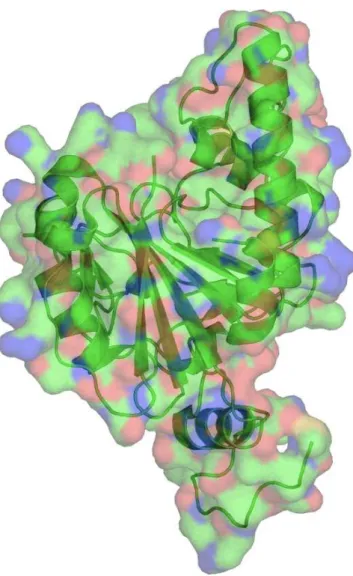
Figure 1.5. Glycosyltransferase A. Generated from the PDB structure using PyMol. The secondary structure is shown in ribbon form with the surface of the protein projected over it. Colours of the surface show the charge distribution of the amino acids on the surface. Green is neutral, red is hydrophobic and blue hydrophilic.
1.4.4 Glycosyltransferases
This large family of enzymes64 is responsible for initiating glycosylation and for elongating glycan chains. Since the substrate specificity of such enzymes is essential to the prediction of glycosylation sites, we briefly review them here. The substrates of these enzymes are varied, but all have in common the transfer of glycans, either monosaccharide or oligosaccharide, to a new substrate. Most of these enzymes are
concerned with chain elongation and in this case the substrate is another glycan. However, receptor substrates can be lipids, peptides, small molecules or DNA. The donor substrates are also varied, for example, dolichol and other lipids. In general, the specificity of glycosyltransferases is such that one enzyme catalyses the formation of one glycosidic linkage e.g. glycosyl transferase A (figure 1.5). However, in several cases multiple enzymes catalyse formation of the same glycosidic linkage. Examples of this are the fucosyltransferases III-VIII, which catalyse the same alpha 1-3 linkage to attach fucose to N-acetyllactoseamine65. There are also rare cases where a single enzyme is capable of forming more than one type of glycosidic linkage, e.g., the case of fucosyltransferase III that can catalyse formation of alpha 1-3 linkages as well as alpha 1-4 linkages. There are also enzymes, which have more than one active site.
1.4.5 N-Linked Glycosylation
In this thesis, one of the major objectives is prediction of both types of glycosylation site: N-linked and O-linked. Here and in the following sections we introduce both in some detail. This provides some context to our work and highlights the significance of the modifications. N-linked glycosylation62,55 is the addition of an oligosaccharide to Asn. This occurs at the consensus sequence Asn Xxx Ser/Thr,55 where the Xxx is anything except Pro. This sequence is necessary, but not sufficient, for glycosylation. N-linked glycosylation takes place co-translationally in the lumen of the ER. Initially, the glycan is pre-assembled on a lipid dolichol molecule55, which acts as a scaffold. This molecule is synthesised on the inner surface of the membrane of the ER, beginning with the transfer of GlcNAc-P to the lipid-like precursor Dolichol-P. 14 sugars are added to dolichol. Oligosaccharyltransferase attaches this glycan precursor molecule to Asn. The transfer to Asn takes place at the consensus sequence found in a
protein which is undergoing synthesis and transport through the membrane into the lumen of the ER. Oligosaccharyltransferase is a multi-subunit protein complex, which is embedded in the ER membrane. The glycan precursor is transferred to Asn as the protein emerges into the lumen of the ER55.
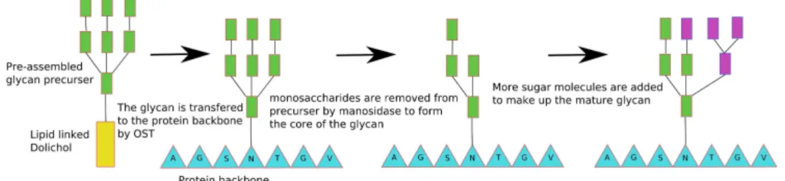
Within the lumen of the ER the oligosaccharide is trimmed of some of its constituent monosaccharides66 (figure 1.6). Glucosidase I and II remove the first two Glc residues. Subsequently, a mannose residue is removed by alpha-mannosidase. This appears to be an important control step for the folding process of the protein with the assistance of chaperone proteins. The oligosaccharides assist in keeping the protein in solution during and after the folding process, thereby, indirectly assisting the function of the chaperone proteins. The chaperones are known to bind to specific points on the immature glycan, thus targeting incorrectly folded proteins for degradation. Once in the Golgi body, alpha mannosidase removes up to a further four mannose residues66, leaving Man5GlcNAc2. This structure forms the basis for all other N-linked glycan chains. There are often some glycans that escape some of these precursor steps.
Figure 1.6. The synthesis and maturation of N-glycans. Green residues represent mannose, purple rectangles are other sugars of unspecified identity, amino acids are shown by blue triangles and the large yellow rectangle is a lipid dolichol molecule.
These are expressed as oligomannose, and cannot form complex or hybrid glycan types. The trimming of glycan precursors only occurs in multi-cellular organisms. In
yeast, for example, extra mannose residues are added to the glycan where in multi-cellular organisms they would be removed.
There are several types of glycan that can be constructed in the Golgi body. The Golgi body contains many specific glycosidases and glycosyltransferases capable of adding or removing different sugars to produce high mannose, hybrid or complex glycan types. All N-linked glycans have a trimannosyl core structure (Man3GlcNAc2). This is the base for many types of linear or branched oligosaccharide. High mannose type oligosaccharides contain between five and nine mannose residues attached to the GlcNAc residues within the trimannosyl core structure. The complex oligosaccharide type does not contain any mannose residues outside of the core structure. Characteristically complex glycans have a disaccharide GlcNAc(beta1-4)Gal attached to the trimannosyl core. This may be a repeating unit or the base for the build up of a complex structure with two, three or four branches. These structures are produced by the stepwise addition of monosaccharides by various glycosyltransferases. Hybrid oligosaccharides possess features of both complex and high mannose type oligosaccharides.
1.4.5.1 Function of N-glycans
As well as assisting in the protein folding process67, N-linked glycans have a number of well documented functions54,68. They have other structural roles in maintaining the conformations of proteins in the appropriate state, as well as preventing non-specific interactions and assisting in the orientation of cell surface molecules. N-linked glycans are important as cell adhesion molecules and for protein signalling, e.g., blood group determinants are oligosaccharides, which can either be N-linked or O-linked glycans.
They also play a role in the serum clearance of proteins.
1.4.6 O-Linked Glycosylation
There are several types of O-linked glycosylation, characterised by the glycan binding to an oxygen atom with an alpha glycosidic linkage. We discuss the common types and their function concentrating on mucin type glycosylation, which is central to the section of this work on predicting glycosylation.
1.4.6.1 O-GalNAc or mucin type modification
Mucin type glycoproteins63,64,69 are usually large molecules (typically greater than 200kDa), which are heavily glycosylated at clusters of Ser and Thr residues, to the extent that one in three amino acids may be glycosylated. The glycan chains that are added to these proteins are varied in composition and structure. These proteins exhibit regions of tandem repeats of variable length70. These contain numerous glycosylation sites and are usually replete with Pro residues, which encourage glycosylation64. Mucin glycoproteins are often secreted or embedded in the membrane. Membrane based glycoproteins mediate cellular adhesion and are involved in cellular signalling. Secreted mucins contribute to the mucosal defences of the body, and are one of the key ingredients in mucosal secretions, giving them their viscosity. O-linked glycans are synthesised in the Golgi body. The synthesis consists of the stepwise addition of monosaccharides to the oligosaccharide chain by glycosyltransferases. There is no trimming and reassembly of the glycan after synthesis unlike N-linked glycans. Whilst O-linked glycans can be long and complex structured oligosaccharides, they can also be short and relatively simple. Most commonly, the monosaccharides GalNAc, GlcNAc, Gal, Fuc, and sialic acid are found in O-linked glycans, although others have
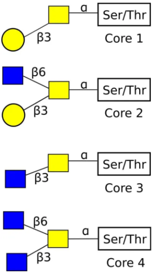
been observed. In contrast to N-linked glycans, O-linked oligosaccharides have less branching in the structure, being based on a biantennary (two branched) core. O-glycans may be classified by the core structure, which falls into one of eight types (see figure 1.7). The synthesis of all mucin type glycans begins with the attachment of GalNAc to either Ser or Thr. This is catalysed by polypeptide-N-acetyl-galactosaminyltransferase. This produces the Tn epitope GalNAcα1-Ser/Thr. This can then be sialylated by α-2,6-sialyltransferase to give sial Tn. This disaccharide cannot be extended further. Alternatively the GalNAc can be extended to form one of the core glycan structures detailed above63. The core structures may be elongated by the further addition of monosaccharides, or the core can be substituted for by a terminal monosaccharide, e.g. Fuc or sialic acid.
Figure 1.7. The four most common O-Glycan core structures. Symbols follow standard conventions as in reference 66. Here yellow circles are Galactose, yellow squares are GalNAc, and blue squares are GlcNAc.
The different core structures tend to be expressed in different structures in different concentrations. The core glycans can be further built upon to synthesize complex glycans of varying structure.
1.4.6.2 Functions of O-linked mucin glycans
Mucin type O-linked oligosaccharides have been implicated in a wide range of functions71. They take a role in the protection of the body against disease. Mucins are produced at biological membranes. The physical properties of these molecules enable them to protect the underlying epithelial cells from infection by bacteria and from extreme environments, e.g., the acidic conditions in the stomach. They provide lubrication, e.g., in the respiratory tract, and act as anti-adhesins, keeping lumen opposing surfaces from sticking together. Mucin glycans are ligands for selectins, mediating the leukocyte homing during the inflammatory response. Mucins can also act as an antifreeze.
Mucins play an important role in bacterial adhesion. Many pathogenic bacteria bind to O-linked oligosaccharides. Thus, this can hinder or occasionally enhance infection. Some species of gut bacteria use mucin proteins as a sole energy source. O-linked glycans also play an important role in sperm-egg recognition and binding. O-linked oligosaccharides are also carried by several types of haemopoietic and immune system cells. They prevent the agglutination of leukocytes both to themselves and to endothelial cells. There are dramatic changes to the glycosylation of T cells during maturation and activation, and oligosaccharides play a role in the interactions between T-cells and B-lymphocytes. Many less common O-glycan modifications also occur within the ER and Golgi. O-mannosylation is a common type of glycosylation in the
brain of mammals and important for binding laminin to the extra-cellular matrix. Alpha linked mannosylation is a common glycosylation of proteins. Initially mannose is added to Ser/Thr by a mannosyltransferase, which is unique to this pathway, as are the subsequent N-acetylglucosaminyltransferases.
1.4.7 Glycosylation of cytosolic and nuclear proteins
Cytoplasmic and nuclear proteins often undergo multiple additions of β-O-GlcNAc72. In addition to mucin glycosylation, we also included cytosolic and nuclear glycosylation sites in our prediction experiments. So we review their structure and function here, to show the benefit of their prediction. These molecules are added as lone monosaccharides, with no further elongation. This type of modification is present across a wide variety of species, including almost all eukaryotes and protozoa, as well as fungi, plants and animals. The modification also occurs on viral proteins. These proteins are often also phosphorylated, and this modification has factors in common with phosphorylation. The O-GlcNAc modifications often occur at sites similar to those modified by phosphokinases and O-GlcNAc modifications are reversible. The composition of occupied GlcNAc sites on a given set of proteins is dynamically changing in response to cell signalling and the various stages of the cell cycle. The interplay between phosphorylation and glycosylation is important in many of the regulatory processes in the cell.
The modification of proteins with O-GlcNAc occurs post translationally and is carried out by the highly conserved enzyme β-N-acetylglucosaminyltransferase, which is itself glycosylated and phosphorylated, probably to regulate its activity. This enzyme occurs in most species and has 85% homology across species. O-GlcNAc