A Dynamic Integer Count Data Model
for Financial Transaction Prices
Roman Liesenfeld University of Pittsburgh Winfried Pohlmeier∗ University of Konstanz CoFE, ZEW February 2003 Abstract
In this paper we develop a dynamic model for integer counts to capture the dis-creteness of price changes for financial transaction prices. Our model rests on an autoregressive multinomial component for the direction of the price change and a dy-namic count data component for the size of the price changes. Since the model is capable of capturing a wide range of discrete price movements it is particularly suited for financial markets where the trading intensity is moderate or low as for most Euro-pean exchanges.
We present the model at work by applying it to transaction data of the Henkel share traded at the Frankfurt stock exchange over a period of 6 months. In particular, we use the model to test some theoretical implications of the market microstructure theory on the relationship between price movements and other marks of the trading process.
JEL classification: C22, C25, G10
Keywords: Autoregressive conditional multinomial model; GLARMA; transaction prices; count data; market microstructure
∗Corresponding author: Department of Economics, Box D124, University of Konstanz, 78457
Kon-stanz, Germany. Tel.: +49-7531-88-2660, Fax.: -4450, e-mail: [email protected]. An earlier version of this paper has been presented at seminars in Helsinki, Munich (SFB386) and Ottobeuren. For helpful comments and suggestions we like to thank Bernd Fitzenberger, Nikolaus Hautsch, Michael Schr¨oder, Neil Shepard, Gerd Ronning and Timo Ter¨asvirta. Nikolaus Hautsch also helped us substan-tially to set up the database. Financial support is gratefully acknowledged by the Center of Finance and Economics (CoFE) of the University of Konstanz.
1
Introduction
Financial transaction data, often called ultra high frequency data, are marked by two main features: the irregularity of time intervals and the discreteness of price changes. Based on the seminal work by Russell and Engle (1998) and Engle (2000), a large body of studies has been centered around the further development of autoregressive conditional duration (ACD) models in order to characterize the transaction intensities. This paper is concerned with appropriately modelling the discreteness of the price process at the transaction level within a count data framework. While previous approaches to model discrete transaction price changes are more suitable for the case of only a few outcomes of the price change, the model we propose is particularly designed for markets where price changes take on a longer range of integer values. This is the case of most assets traded at European asset markets because they have a considerably lower transaction intensity than, for instance, the shares traded at the NYSE.
Since transaction price changes are quoted as multiples of a smallest divisor (called a ’tick’), the use of continuous distributions to characterize price changes is far from be-ing appropriate in particular for markets with high transaction intensities. Accordbe-ingly, Hausman, Lo, and MacKinlay (1992) proposed an ordered probit model with conditional heteroscedasticity to analyze stock price movements at the NYSE. The same approach is used by Bollerslev and Melvin (1994) to model the bid-ask spread at FX-markets and by Gerhard, Hess, and Pohlmeier (1998) for price movements of the BUND future traded at the LIFEE. Contrary to the older rounding approaches proposed by Ball (1988), Cho and Frees (1988) and Harris (1990) conditioning information can be incorporated in the ordered response models quite easily. A drawback of the ordered probit approach is that the parameters result from a threshold crossing latent variable model, where the under-lying continuous latent dependent variable has to be given some more or less arbitrary economic interpretation (e.g., latent price pressure). Moreover, since the parameters are only identified up to a factor of proportionality, the estimates of the moments of the latent price variable are only identifiable using additional identifying restrictions.1
An alternative to the ordered response models is the autoregressive conditional multino-mial (ACM) model proposed by ?. Similar to the ordered response models this approach also rests on the assumption that the distribution of observed transaction price changes is discrete with a finite number of outcomes. A drawback of the ACM model is the necessity that all potential outcomes have to occur in the sample period to guarantee the identifica-tion and estimaidentifica-tion of the true dimension of the multinomial process. In the multinomial approaches as well as in the ordered response models, the number of parameters increases
with the outcome space. As long as one is not willing to categorize the outcomes at the expense of a loss of information, both approaches are more suited for the empirical analysis of financial markets which are characterized by a limited number of discrete price changes. Using examples from the Frankfurt stock market, Hautsch and Pohlmeier (2002) point out that the transaction price process of assets traded at typical European exchanges reveals a comparatively wide range of discrete price movements. We therefore propose in the sequel a model that does not suffer from the drawbacks of the discrete response models sketched above. We propose a dynamic model which is based on a probability density function for an integer count variable and which can be interpreted as a count data hurdle model. Our integer count hurdle (ICH) model is closely related to the components approach by Rydberg and Shephard (2002) who suggests decomposing the process of transaction price changes into three distinct processes: a binary process indicating whether a price change occurs from one transaction to the next, a binary process indicating the direction of the price change conditional on a price change having taken place and a count process for the size of the price change conditional on the direction of the price change. By incorporating the above mentioned two binary processes into a trinomial ACM model (no price change or price movement downwards or upwards) and using a count process for the size of the price change based on a dynamic count data specification, our approach is more parsimonious than the one proposed by Rydberg and Shephard. The distribution of price changes used is that of a count data hurdle model extended for the domain of negative integer counts. For both components of the price process, the dynamics are modelled using a generalized ARMA specification. This procedure is computationally less burdensome than the dy-namic ordered probit model ?, which is based on an ARMA specification for the latent price variable.
Our model can be extended in many respects. Inclusion of contemporaneous marks of the transaction price process as conditioning information (e.g. transaction time and volume) can generate insights into the validity of various hypotheses of market microstructure the-ory. In our empirical application of the ICH model, we will analyze the distribution of price changes conditional on transaction time and volume. Our model can also serve as a building block for the joint process of transaction price and transaction times. In this sense, our approach is more flexible than the competing risks ACD model by Bauwens and Giot (2002), which focuses on the direction of the price process whereby neglecting information on the size of the price changes.
The paper is organized as follows. We first introduce the ICH model in its basic form as a time series model. We then extend the model by introducing transaction volume and
transaction time, which play a central role in the literature on market microstructure, and finally, we test some popular hypotheses of market microstructure theory. Our empiri-cal results are based on transactions data of the Henkel shares quoted on the electronic XETRA platform at the Frankfurt stock exchange.2 Our sample period includes 28,165 transactions within a time period of 6 months from July 1 until December 30, 1999. The smallest possible price change is 0.01 Euro. During this sample period, the trading hours were changed. Until September 17th, XETRA trading took place between 8.30 and 17.00. Starting on September 21st, trading time was changed to 9.00 to 17.30. Since the dynamics of transaction prices at the beginning and the end of the trading day differ from the be-havior of prices on the rest of the trading day, we exclude transactions occuring before 9.30 and after 16.00. This reduces the sample to 20,051 transactions. Figure 1 of the appendix depicts the histogram of the transaction price changes. Rather typical for transaction data is the large fraction of zero price changes (around 34%). The remaining observations are equally distributed between positive and negative price changes (approximately 33% for each), so that the empirical distribution is close to being symmetric.
2
The Hurdle Approach to Integer Counts
Consider a sequence of transaction prices{P(ti), i: 1→n} observed at times {ti, i: 1→
n} . Let {Yi, i : 1 → n} be a sequence of price changes, where Yi = P(ti)−P(ti−1) is
an integer multiple of a fixed divisor (tick), then Yi ∈ Z. Our interest lies in modeling
the conditional distribution of the discrete price changes Yi
¯
¯Fi−1 , where Fi−1 denotes
the information set available at the time transactionitakes place. For this we generalize the hurdle approach proposed by Mullahy (1986) and Pohlmeier and Ulrich (1995) for the Poisson and the negative binomial distribution respective to negative counts. The basic idea of this approach is to decompose the overall process of transaction price changes into three distinct partial processes. The first process determines the sign of the process (positive price change, negative price change, or no price change) and will be specified as a dynamic multinomial response model. Given the direction of the price change, a count data process determines the size of positive and negative price changes. This yields the following structure for the p.d.f. ofYi
¯ ¯Fi−1: Pr(Yi =yi ¯ ¯Fi−1) = Pr(Yi<0 ¯ ¯Fi−1)Pr(Yi =yi¯¯Yi <0,Fi−1) if yi<0 Pr(Yi= 0 ¯ ¯Fi−1) if yi= 0 Pr(Yi>0¯¯Fi−1)Pr(Yi =yi¯¯Yi >0,Fi−1) if yi>0 . (2.1)
The process driving the direction of the price changes is represented by Pr(Yi <0
¯ ¯Fi−1),
Pr(Yi = 0
¯
¯Fi−1) and Pr(Yi >0¯¯Fi−1) , while Pr(Yi =yi¯¯Yi <0,Fi−1) and Pr(Yi =yi¯¯Yi >
0,Fi−1) denote the two processes for the size of the price changes conditional on the price
direction. Note that Pr(Yi =yi
¯
¯Yi >0,Fi−1) is a process defined over the set of strictly
positive integers and Pr(Yi = yi
¯
¯Yi < 0,Fi−1) is the corresponding p.d.f. for strictly
negative counts. This decomposition allows us to model the stochastic behavior of the transaction price changes successively.
We follow Mullahy’s (1986) idea by modelling the size of positive price changes as a truncated-at-zero count process.3 Letf+(·) be the p.d.f. of a standard count data
distri-bution, then the p.d.f. for the size of positive price changes conditional on the fact that the prices are positive is a truncated-at-zero count data distribution:
Pr(Yi =yi ¯ ¯Yi>0,Fi−1) =h+(y i ¯ ¯Fi−1) = f+(yi ¯ ¯Fi−1) 1−f+(0¯¯Fi−1) . (2.2)
The process for the size of negative price jumps is treated in the same way: Pr(Yi =yi¯¯Yi<0,Fi−1) =h−(yi¯¯Fi−1) = f −(−y i ¯ ¯Fi−1) 1−f−(0¯¯Fi−1) , (2.3)
where f−(·) denotes the p.d.f. of a standard count data model. Combining the single
components leads to the p.d.f. for the transaction price changes: Pr(Yi=yi ¯ ¯Fi−1) =hPr(Yi<0¯¯Fi−1)h−(y i ¯ ¯Fi−1)iδi−h Pr(Yi = 0 ¯ ¯Fi−1)iδi0 (2.4) × h Pr(Yi >0 ¯ ¯Fi−1)h+(y i ¯ ¯Fi−1)iδi+ ,
whereδi−= 1l{Yi<0},δi0 = 1l{Yi=0} and δ+i = 1l{Yi>0} are binary variables indicating posi-tive, negative or no price change for transactioni.
A more parsimonious distribution results if one assumes thath−(·) and h+(·) arise from
the same parametric family of probability density functions. Based on this assumption, the stochastic behavior of positive and negative price movements can be summarized in a conditional p.d.f. for the absolute price changes Si = ¯¯Yi¯¯ conditional on the price direction. I.e.: Pr(Si=si ¯ ¯Si>0, Di,Fi−1) =h(si¯¯Di,Fi−1) with Di= −1 if Yi<0, 0 if Yi= 0, 1 if Yi>0 (2.5)
3Alternatively, one could specify the p.d.f. of the transformed countY
i−1 conditional onYi>0 using
a standard count data approach. This approach was adopted by Rydberg and Shephard (2002) in their decomposition model.
where h(·) is the p.d.f. of a truncated-at-zero count data model. For the parsimonious specification, the p.d.f. for a transaction price change is:
Pr(Yi=yi ¯ ¯Fi−1) = Pr(Yi <0¯¯Fi−1)δ−i Pr(Yi= 0¯¯Fi−1)δi0Pr(Yi >0¯¯Fi−1)δi+ (2.6) × h h(|yi| ¯ ¯Di,Fi−1)i(1−δi0) .
In this case, the resulting sample log-likelihood function of the ICH-model consists of two additive components: L= n X i=1 ln Pr(Yi =yi ¯ ¯Fi−1) =Xn i=1 L1,i+ n X i=1 L2,i, (2.7) where: L1,i = δ−i ln Pr(Yi<0 ¯ ¯Fi−1) +δ0 i ln Pr(Yi = 0 ¯ ¯Fi−1) +δ+ i ln Pr(Yi >0 ¯ ¯Fi−1) (2.8) L2,i = (1−δi0) lnh(|yi| ¯ ¯Di,Fi−1). (2.9)
The component PL1,i is the log-likelihood of the multinomial process determining the direction of prices, whilePL2,iis the log-likelihood of the truncated-at-zero count process
for the absolute size of the price change. If there are no parametric restrictions across the two likelihoods, which does not lead to substantial reduction of generality, we can maximize equation (2.7) by separately maximizing equations (2.8) and (2.9). This reduces the computational burden considerably. In the following section, we consider specific functional forms for the p.d.f. for the price direction and the absolute size of the price changes. In a second step, we then extend the model by introducing the trading volume at times between transactions (duration) as conditioning information.
2.1 The Price Direction
The parametric model for the direction of the transaction price change Di = j, (j =
−1,0,1) is taken from the class of logistic ACM (autoregressive conditional multinomial) models suggested by?. In order to formulate the probabilityπji = Pr(Di =j¯¯Fi−1) for the occurrence of price directionj, we use a logistic link function. This leads to a multinomial logit model of the form:
πji = P1exp{αji} j=−1exp{αji}
, j=−1,0,1, (2.10)
where the variableαjicaptures the explanatory variables affecting the price direction prob-abilities. As a normalizing constraint, we useα0i= 0.
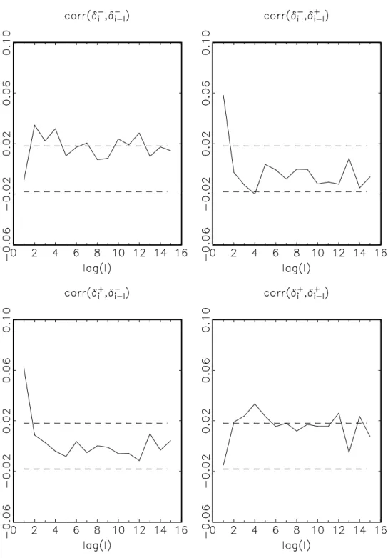
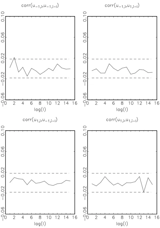
A well known property of transaction price changes is the serial dependence resulting from the bid-ask-bounce. This has to be taken into account when modeling the conditional distribution of price directions. An indicator of the strength of serial correlation in the direction of the price process is given by the sample autocorrelation matrix of the state vector: xi = (x−1i, x1i)0 = (1,0)0 if Y i <0 (0,0)0 if Yi = 0 (0,1)0 if Y i >0, (2.11)
which contains the corresponding auto- and cross-autocorrelation of the statesx−1i=δ−i 1
andx1i =δi+. For a lag length l, the sample autocorrelation matrix is:
Υ(`) =D−1Γ(`)D−1 , l= 1,2, ... , (2.12) with Γ(`) = 1 n−`−1 n X i=`+1 (xi−x¯)(xi−`−x¯)0.
Ddenotes a diagonal matrix containing the standard deviations ofx−1i andx1i. Figure 2
depicts the cross-correlation function up to order 15. The significant, but not very large, first order cross-correlations provide the first empirical evidence for the existence of a bid-ask bounce. The probability of a price reduction is significantly positively correlated with the price increase in the previous period (upper right panel), and, also significantly, a price increase is more likely if a negative price change were to be observed for the previous transaction (lower left panel). Moreover, the autocorrelation-functions for positive price changes and negative price changes reveal that the probability of the price changing in the same direction in successive trades is negligible. However, the positive autocorrelations at longer lags indicate that the bounce effect will be compensated over a longer time horizon, so that the negative serial correlation caused by the bid-ask bounce is a short run phenomenon. In order to capture dynamic behavior for the direction of the prices, the vector of log-odds ratiosαi = (α−1i, α1i)0 = (ln[π
−1i/π0i],ln[π1i/π0i])0 will be formulated
as a multivariate ARMA process:
αi=µ+ p X l=1 Clαi−l+ q X l=1 Alξi−l, (2.13) with {Cl, l : 1 → p} and {Al, l : 1 → q} being matrices of dimension (2×2) with the
elements {c(hkl)}, {ahk(l)} and µ = (µ1, µ2)0. The vector of log-odds ratios is driven by the
martingale differences: ξi = (ξ−1i, ξ1i)0 , with ξji= xji−πji p πji(1−πji) , j=−1,1, (2.14)
which is the standardized state vector xi. In this ACM-ARMA(p,q) specification, the
conditional distribution of the direction of price changes depends on lagged conditional distributions of the process and the lagged values of the standardized state vector. The process is stationary, if all values ofzthat satisfy¯¯I−C1z−C2z2− · · · −Cpzp
¯
¯, lie outside
the unit circle.4
According to the classification of Cox (1981), our model belongs to the class of obser-vationally driven models where time dependence arises from a recursion on the lagged endogenous variable. Alternatively, our model could be based on a parameter driven spec-ification, in which the log-odds ratios αi are determined by a dynamic latent process. However, the estimation and the diagnostics of the latter approach results in a substan-tially higher computational burden for the ACM model. On the other hand, models driven by latent processes are usually more parsimonious than comparable dynamic models based on lagged dependent variables. A comparison of the two alternatives should be the subject of future research.
The log likelihood of the logistic ACM model, the first component of the likelihood of the overall model, takes on the familiar form presented below:
L1 =
n
X
i=1
[δ−i lnπ−1i+δi0lnπ0i+δ+i lnπ1i]. (2.15)
In order to guarantee that a scant number of parameters are estimated,? suggest imposing symmetry restrictions on the autoregressive structure. This approach can be justified by the observed symmetry of the cross-autocorrelation functions of the state variable presented above. In the sequel, we assume that the marginal effect of a negative price change on the conditional probability of a future positive price change is of the same size as the marginal effect of a positive change on the probability of a future negative change. Moreover, we impose the restriction that the impact of a negative change on the probability of a future negative change is the same as the corresponding effect for positive price changes. The symmetry of impacts on the conditional price direction probabilities will also be imposed for all lagged values of the probabilities and normalized state variables. This simplifies the ARMA-specification (2.13) to:
µ= Ã µ1 µ1 ! , Cl = Ã c(1l) c(2l) c(2l) c(1l) ! , Al= Ã a(1l) a(2l) a(2l) a(1l) ! . (2.16)
Following ?, we also set c(2l) = 0, which implies that stocks in the log-odds ratios vanish at an exponential rate determined by the diagonal element c(1l). Although the reasoning
behind these restrictions seems appropriate due to the explorative evidence of the state variable xi, the validity of these restrictions can, of course, be easily tested by standard
ML based tests.
In search of the best specification, we use the Schwarz information criterion to determine the order of the ARMA process. For the selected specification, its standardized residuals will then be subject to diagnostic checks. For the estimates of the conditional expectations and the variances ˆE(xi
¯
¯Fi−1) = ˆπi and ˆVar(xi¯¯Fi−1) = diag(ˆπi)−πˆiπˆ0
i, respectively, the
standardized residuals can be computed as:
υi= (υ−1i, υ1i)0 = ˆVar(xi ¯ ¯Fi−1)−1/2£x i−E(ˆ xi ¯ ¯Fi−1)¤, (2.17)
where ˆVar(xi¯¯Fi−1)−1/2 is the inverse of the Cholesky factor of the conditional variance.
For a correctly specified model, the standardized residuals should be serially uncorrelated in the first two moments with the following unconditional moments: E(υi)=0 and E(υiυ0i)=
I. The null hypothesis of absence of serial (cross-) correlation in υi can be tested by the multivariate version of the Portmanteau statistic presented by Hosking (1980):
Q(L) =n L X `=1 tr£Γυ(`)0Γυ(0)−1Γυ(`)Γυ(0)−1 ¤ , (2.18) where Γυ(`) = Pn
i=`+1υiυi0−`/(n−`−1). Under the null hypothesis, Q(L) is
asymptot-icallyχ2-distributed with degrees of freedom equal to the difference between 4L and the
number of parameters to be estimated.
According to the Schwarz criterion, the ACM-ARMA(1,2) specification turns out to have the best goodness of fit. The estimation results and the results of the diagnostic checks are summarized in Table 1. With the exception of the intercept term µ1 all coefficient estimates are significantly different from zero at the 1% level. The estimated value ofc(1)1
at 0.945 indicates that the process of log-odds ratios αi reveals a high degree of
persis-tence. Regardless of the sign of the price direction, the probability of a price change is comparatively high if the probability of a price change for the previous transaction was high. Note that the probability of a price change can be interpreted as a specific measure of price volatility. In this sense, our finding reflects the typical phenomenon of volatility clustering. Sincea(1)2 = 0.212 is significantly larger than a(1)1 = 0.143, the probability of a negative price change occurring after a positive price change for the previous transaction is larger than the probability of a negative price change following another negative price change. Correspondingly, this also holds for the probability of a positive price change. This finding can be explained by the existence of a bid-ask bounce. Finally, the negative signs for a(2)1 and a(2)2 and the size relation |a(2)1 | < |a(2)2 | indicate that an initial price change will be partially compensated by the next transaction.
With a value of 56.50 for the generalized Portmanteau statisticQ(15), we are not able to reject the null hypothesis of no cross-correlations at the usual significance levels. Compar-atively, for the raw dataxi, the corresponding value of theQ(15) statistic was found to be
611.79. This indicates that the ACM-ARMA specification is well suited in explaining the dynamics of the direction of price changes. This is supported by Figure 3, which depicts the cross-correlation functions of the standardized residualsυ−1i andυ1i. With one exception,
all correlations lie within the 99% confidence band. The means of standardized residuals reported in Table 1 are close to zero, which should be expected from a well specified model. However, the estimated variance-covariance matrix of the standardized residuals deviates slightly from the identity matrix. This may hint to a distibutional misspecification or a misspecification of log-odds ratiosαi, which is not fully compatible with the variation in
the observed variation of price change direction.
2.2 The Size of Price Changes
In order to analyze the size of the non-zero price changes, we use a GLARMA (generalized linear autoregressive moving average) model based on a truncated-at-zero Negbin distri-bution. Similar to the ACM, model the dynamic structure of this count data model rests on a recursion on lagged observable variables. A comprehensive description of this class of models can, for instance, be found in Davis, Dunsmuir, and Streett (2001). Note, that the time scale for absolute price changes is different from the one of the ACM model for the direction of the price changes, which is defined on the ticktime scale. Letu be a random variable following a Negbin distribution with the p.d.f. 5
f(u) = Γ(κ+u) Γ(κ)Γ(u+ 1) à κ κ+ω !κà ω ω+κ !u , u= 0,1,2, ... , (2.19) with E(u) =ω >0 and Var(u) =ω+ω2/κ. The overdispersion of the Negbin distribution
depends on parameter κ > 0, where as κ → ∞, the Negbin converges to a Poisson distribution. For the truncated-at-zero Negbin distribution, we obtainh(u) = f(u)/[1−
f(0)], (u = 1,2,3, ...), with f(0) = [κ/(κ+ω)]κ. This flexible class of distribution will
be used to model the size of the non-zero price changes conditional on filtrationFi−1 and
price directionDi. Thus for Si|Si >0, Di,Fi−1, we assume the following p.d.f.:
h(si¯¯Di,Fi−1) = Γ(κ+si) Γ(κ)Γ(si+ 1) Ãh κ+ωi κ iκ −1 !−1à ωi ωi+κ !si , si = 1,2, ... , (2.20)
with the conditional moments: E(Si|Si >0, Di,Fi−1) = µSi = ωi 1−ϑi (2.21) Var(Si|Si >0, Di,Fi−1) = σ2Si = ωi 1−ϑi − ω2 i (1−ϑi)2 ³ ϑi− 1−ϑi κ ´ , (2.22) where ϑi = [κ/(κ+ωi)]κ. In this specification, both mean and variance are monotonic
increasing functions of the parameter ωi that is assumed to capture the variation of the
conditional distribution depending onDi and Fi−1.
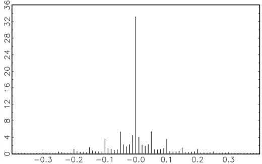
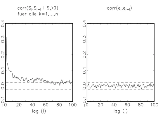
Volatility clustering of asset returns is a well-known property, particularly for high fre-quency data. Figure 4, (left panel), shows the autocorrelation function of the absolute price changes Si|Si >0. As for the case of equidistant return rates, we observe volatility
clustering for the absolute price changes at the transaction level. In order to take into ac-count the dynamics ofSiwe follow Rydberg and Shephard (2002) and impose a GLARMA
structure on lnωi as follows:6 lnωi =β1Di+β2Di−1+λi, with λi=γ0+ p X l=1 γlλi−l+ q X l=1 δlεi−l . (2.23)
Here, the standardized absolute price change, εi = Siσ−µSi
Si , drives the ARMA process in
λi. The inclusion of Di is to capture potential differences in the behavior of the absolute price changes depending on the direction of the price process. Thus, a negativeβ1 implies
that with negative price changes (Di = −1) large absolute price changes are more likely
to occur than with positive price changes (Di = 1). If one interprets the absolute price changes as an alternative volatility measure, this asymmetry reflects a kind of leverage ef-fect, where downward price movements imply a higher volatility than upward movements.7
The additional termDi−1 allows for a dynamic variant of the leverage effect.
For the estimation of parameters of the GLARMA(p,q) model, equations (2.20) to (2.23), we maximize the log-likelihoodL2 =Pni=1(1−δ0
i) lnh(si
¯
¯Di,Fi−1) using the BHHH
algo-rithm. For the ACM specification, we use the Schwarz information criterion to determine the optimal order ofpandq. The diagnostic checks are based on the standardized residuals
ei = Siσ−ˆ µˆSi Si
. (2.24)
For a correctly specified model the residuals evaluated at the true parameter values should be uncorrelated in the first two moments with E(ei) = 0 and E(e2i) = 1.
6Similar to the alternative specification discussed in the context of the ACM model one could also specify a dynamic latent process forωi. See Zeger (1988) and Jung and Liesenfeld (2001) for examples.
The estimation results for the model of the absolute price changes are reported in Table 2. The GLARMA(2,3) specification shows the best goodness of fit in terms of the Schwarz criterion. The two left columns contain the results of the specification of an asymmetric price effect model allowing for a leverage effect. For reasons of comparison we present the estimates for a specification excluding asymmetric price effects in the columns on the right. The parameters for the ARMA components and the dispersion parameterκ−1/2are statistically different from zero, whileDi and Di−1 have no significant impact on the size
of the price changes. This finding is in contrast to previous results provided by Rydberg and Shephard (2002). They find a leverage effect for transaction prices of the IBM share traded at the NYSE. The dispersion parameter κ−1/2 being significantly different from
zero implies that we have to reject the null of a truncated-at-zero Poisson distribution in favor of a Negbin distribution. The implicit estimates for the two roots of the AR com-ponents are for both, the symmetric and asymmetric model, 0.9982 and 0.8795, so that stationarity is guaranteed. However, the larger of the two roots is close to 1 implying that the GLARMA model reveals a strong persistence in the non-zero absolute price changes. The value of Box-Pierce statisticsB(τ) for the standardized residualsei reported in Table
2 for lag length τ = 20,50,100 indicates that the GLARMA(2,3) specification is able to explain the observed autocorrelation in the absolute price changes almost completely. The corresponding values of B(τ) for the observed transaction data Si|Si >0 are 3176, 3861
and 4339 for τ = 20,50,100. Figure 4, (right panel), depicts the autocorrelations for ei
which lie well within the confidence band. Finally, the means for ei and e2i reported in
Table 2 do not provide any evidence of a potential misspecification due to the Negbin assumption or the GLARMA specification.
3
Transaction Price Dynamics and Market Microstructure
One of the fundamental questions of the market microstructure theory of financial markets is concerned with the determinants of the price process and the specific role of the insti-tutional set-up.8 Generally, the goal is to figure out how new price relevant information
affects the price process. Approaches based on the rational expectation hypothesis typ-ically assume some kind of heterogeneity of information among the market participants, where information about the transaction process generally leads to successive revelations of price information. This leads to empirically testable hypotheses about the process of transaction price changes and other marks of the trading process, such as transaction in-tensities and transaction volume.
Provided that short-selling is infeasible, Diamond and Verrecchia (1987) infer that longer times between transactions can be taken as a signal that the existence of bad news im-plies negative price reactions. The absence of a short selling mechanism prevents market participants from profiting by exploiting the negative information through corresponding transactions. Therefore, one can expect that low transaction rates (longer times between transactions) are associated with higher volatility in the transaction price process and vice versa.
Easley and O’Hara (1992) provide an alternative explanation of the relationship between transaction intensities and transaction price changes. In their model, higher transaction rates occur when a larger share of informed traders is active, which is anticipated by less informed traders. Consequently, the price reacts more sensitively when the market is marked by high transaction intensities than at times when the transaction intensity is low. Contrary to Diamond and Verrechia, Easley and O’Hara predict a negative relationship between transaction times and volatility.
Similar predictions about the link between price dynamics and transaction volume result from the model proposed by Easley and O’Hara (1997). In their model, informed market participants try to trade comparatively large volumes per transaction in order to profit from their current informational advantage. It is assumed that this advantage exists only temporarily. The occurrence of those large transactions are seen by uninformed traders as evidence for new information. Hence, one can expect that the price reacts to larger orders more sensitively than to smaller ones. In general, price volatility should be larger when larger trading volumes are observed.
A further theoretical explanation for the positive association between trading volume and volatility goes back to the mixture of distribution model of Clark (1973) and Tauchen and Pitts (1983). In a standard set-up of the model, the positive association results from a joint dependence on the news arrival rate.9
A suitable framework for quantifying the relationship between transaction price changes and other marks of the trading process, such as trading volumes and transaction rates, is their joint distribution. LetZi be the vector representing the marks of the trading process
with the joint p.d.f. Pr(Yi = yi, Zi|Fi(−y,z1)) for transaction price changes and the marks
conditional on partial filtration.
Without any loss of generality, the joint p.d.f. can be decomposed into the p.d.f. of the price changes conditional on the marks and the marginal density of the marksf(Zi|Fi(−y,z1)):
Pr(Yi =yi, Zi|Fi(−y,z1)) = Pr(Yi=yi|Zi,Fi(−y,z1))f(Zi|Fi(−y,z1)), (3.1)
Obviously, the p.d.f. of the ICH model can be used to specify the conditional p.d.f. of the price changes. In the following we extend the ICH model by introducing the transaction rate and trading volume as conditioning information.
Let Ti be the time between transaction i−1 and i (measured in seconds) and Vi the transaction volume (measured as the number of shares). For the ACM component we extend the ARMA specification of the log-odds ratios (2.13) as follows:
αi =µ+ p X l=1 Clαi−l+ q X l=1 Alξi−l+gt1lnTi+gv1lnVi+gt2lnTi−1+gv2lnVi−1, (3.2)
where symmetry restrictions, similar to those imposed on matrices A and C in equation (2.16), are imposed on the parameter vectorsgt1,gv1,gt2 and gv2. Imposing these
restric-tions means, for example, that an increase in the transaction intensity Ti has the same
impact on the probability of a positive price response as on a negative one.
This restriction contradicts the implication of the theoretical hypothesis of Diamond and Verrecchia (1987) who predict a negative correlation between price changes and the time between transactions. Hence, one would expect asymmetric effects on the probabilities of a certain price reaction. However, tests for an asymmetric price response could not reject the null hypothesis of symmetric price reactions.
In a similar way, the transaction rate and the transaction volume can be introduced as conditioning information into the model for the size of the price changes:
lnωi=βt1lnTi+βv1lnVi+βt2lnTi−1+βv2lnVi−1+λi (3.3) with λi =γ0+ p X l=1 γlλi−l+ q X l=1 δlεi−l.
Since the direction of the price changes had no significant impact in the specification (2.23), we refrain from considering this covariate as an additional covariate in our GLARMA model (3.3). Note that our interpretation of the parameter estimates does not explic-itly rest on a structural theoretical model for the joint process of price changes, volume and transaction rates. Equations (3.2) and (3.3) rather reflect ad-hoc assumptions with respect to the probability function of the price changes conditional on volume and trans-action rate. Correspondingly, the estimated relations cannot be interpreted as structural economic relations. The dynamic ICH model, rather should serve as an instrument for capturing and quantifying the relationship between important marks of the trading
pro-cess. Consequently, this allows us to shed light on the empirical relevance of the theoretical implication sketched above.
Tables 3 and 4 contain the estimation results for the ICH model that has been extended to include transaction rates and trading volume as additional covariates. For the two sub-models, we have chosen the same order of the process that was found to be optimal for the pure time series specification. For the direction of the price process (Table 3) both log trading volumeVi and the log time between transactionsTi have a significantly
positive impact on the log-odds ratios αi (i.e., the probability that the transaction price
changes increases with the size of the transaction volume and the time between transac-tions). Since the probability of a non-zero price change can be interpreted as a specific measure of price volatility, it implies that low transaction rates go along with higher price volatility. This provides empirical support for the implications of the model proposed by Diamond and Verrecchia (1987), where no transactions indicate bad news, which contra-dicts the theoretical implications of by Easley and O’Hara (1992), where no transactions indicate lack of news in the market. Our finding, that high transaction volumes are posi-tively corrected with volatility, is consistent with the implication of the model proposed by Easley and O’Hara (1997), where large volumes correspond to the existence of additional news in the market. Moreover, signs of the estimated coefficientsgv2 and gt2 reveal that the impact of volume and transaction rate on the vector of log-odds ratios will be partly compensated for by the subsequent transaction. Finally, the value of the Schwarz criterion greatly improves the fit when volume and transaction rate are included. However, both the Portmanteau statisticsQ(15) and the sample moments of the standardized residuals indicate that neither the dynamic properties nor the distributional characteristics of the model are captured completely. Our empirical results for the direction of the price changes are in accordance with those put forth Rydberg and Shephard (2002). In particular, they also find a positive impact of transaction volume and time between transactions on the activity of transaction prices.
Table 4 reports the estimation results for the size of the non-zero price changes for the GLARMA model. Adding volume and transaction rate, the specification for the ACM component leads to a substantial improvement of the first, in terms of the Schwarz crite-rion. To a large extent, the reported diagnostics on the residuals confirm that the dynamic properties and the distributional properties can be explained by the model. Again, volume and transaction rate have a positive impact on the size of the price changes. Since the size of the price changes as well as the probability of a non-zero price change are volatility mea-sures, our previous conclusions based upon the ACM component regarding the empirical confirmation of various implications from market microstructure theory are confirmed.
4
Conclusions
In this paper, we introduce a new approach to analyzing transaction price movements in financial markets. It relies on a hurdle count data approach that has been extended to include negative counts. The parsimonious form of our model consists of two processes: a process for the price direction and one for the size of the price movement. Our approach is particularly suited for financial markets with fairly low transaction intensities.
For the XETRA-trading of Henkel shares, we show that our model is suited for testing various implications of market microstructure theory without claiming that it is superior to alternative approaches. In order to assess the potential of our approach, the model has to be subjected to intensive diagnostic checks. Comparative studies with respect to the forecasting properties of various approaches and applications to other financial assets and to exchanges with different trading platforms should provide more insights into the potential applicability of our approach. Alternatively, the quality of the model could be assessed by using it as the basis for a trading strategy. Finally, the ICH model should be embedded into a joint model of the transaction price movements and trading times.
References
Andersen, T. G.(1996): “Return Volatility and Trading Volume: An Information Flow Interpretation of Stochastic Volatility,”Journal of Finance, 169-204, 169–231.
Ball, C. (1988): “Estimation Bias Induced by Discrete Security Prices,” Journal of Finance, 43, 841–865.
Bauwens, L.,andP. Giot(2002): “Asymmertic ACD Models: Introducing Price Infor-mation in ACD Models,” Core Discussion Paper 9844, revised version, January 2002.
Bollerslev, T.,andM. Melvin(1994): “Bid-Ask Spreads and Volatility in the Foreign Exchange Market - An Empirical Analysis,” Journal of International Economics, 36, 355–372.
Cameron, A. C.,andP. K. Trivedi(1998): Regression Analysis of Count Data. Cam-bridge University Press, CamCam-bridge.
Cho, D. C., and E. W. Frees (1988): “Estimating the Volatility of Discrete Stock Prices,”Journal of Finance, 43, 451–466.
Clark, P. K. (1973): “A Subordinated Stochastic Process Model with Finite Variance for Speculative Prices,”Econometrica, 41, 135–155.
Cox, D.(1981): “Statistical Analysis of Time Series: Some Recent Developments,” Scan-dinavian Journal of Statistics, 8, 93–115.
Davis, R., W. Dunsmuir, and S. Streett (2001): “Observation Driven Models for Poisson Counts,” Discussion paper, Colorado State University, Fort Collins.
Diamond, D. W., and R. E. Verrecchia (1987): “Constraints on Short-Selling and Asset Price Adjustment to Private Information,” Journal of Financial Economics, 18, 277–311.
Easley, D., and M. O’Hara (1992): “Time and the Process of Security Price Adjust-ment,”Journal of Finance, 47, 577–607.
Easley, D., and M. O’Hara (1997): “Price, Trade Size, and Information in Securities Markets,”Journal of Financial Economics, 19, 69–90.
Engle, R.(2000): “The Econometrics of Ultra-High-Frequency Data,”Econometrica, 68, 1, 1–22.
Gerhard, F., D. Hess, andW. Pohlmeier(1998): “What a Difference a Day Makes: On the Common Market Microstructure of Trading Days,” Discussion Paper 98/01, CoFE, Konstanz.
Harris, L.(1990): “Estimation of Stock Variances and Serial Covariances from Discrete Observations,” Journal of Financial and Quantitative Analysis, 25, 291–306.
Hausman, J. A., A. W. Lo, and A. C. MacKinlay (1992): “An Ordered Probit Analysis of Transaction Stock Prices,”Journal of Financial Economics, 31, 319–379.
Hautsch, N.,andW. Pohlmeier(2002): “Econometric Analysis of Financial Transac-tion Data: Pitfalls and Opportunities,”Allgemeines Statistisches Archiv, 86, 5 – 30.
Hosking, J.(1980): “The Multivariate Portmanteau Statistic,”Journal of the American Statistical Association, 75, 602–608.
Jung, R., and R. Liesenfeld(2001): “Estimating Time Series Models for Count Data Using Efficient Importance Sampling,”Allgemeines Statistisches Archiv, 85, 387–407.
Mullahy, J.(1986): “Specification and Testing of Some Modified Count Data Models,”
Journal of Econometrics, 33, 341–365.
Nelson, D.(1991): “Conditional Heteroskedasticity in Asset Returns: A New Approach,”
Journal of Econometrics, 43, 227–251.
O’Hara, M.(1995): Market Microstructure Theory. Blackwell Publishers, Oxford.
Pohlmeier, W.,andF. Gerhard(2001): “Identifying Intraday Volatility,” in Beitr¨age Zur Mikro- und Zur Makro¨okonomik, Festschrift Zum 65. Geburtstag Von Hans J¨urgen Ramser, ed. by S. Berninghaus,and M. Braulke. Springer.
Pohlmeier, W., and V. Ulrich (1995): “An Econometric Model of the Two-Part Decision Process in the Demand for Health,” Journal of Human Resources, 30, 339– 361.
Russell, J. R., and R. F. Engle (1998): “Econometric Analysis of Discrete-Valued, Irregularly-Spaced Financial Transactions Data Using a New Autoregressive Conditional Multinomial Model,” Discussion paper, presented at Second International Conference on High Frequency Data in Finance, Zurich, Switzerland.
Rydberg, T., and N. Shephard (2002): “Dynamics of Trade-by-Trade Price Move-ments: Decomposition and Models,” Discussion paper, Nuffiled College, Oxford Uni-versity, will be published in Journal of Econometrics.
Tauchen, G. E., and M. Pitts(1983): “The Price Variability-Volume Relationship on Speculative Markets,” Econometrica, 51, 485–505.
Zeger, S. (1988): “A Regression Model for Time Series of Counts,” Biometrika, 75, 621–629.
A
Tables
Table 1: ML estimates of the logistic ACM-ARMA(1,2)-model for the direction of price changes
parameter estimate std. dev. parameter estimate std. dev.
µ1 .001 .001 c(1)1 .945 .011 a(1)1 .143 .015 a(1)2 .212 .015 a(2)1 −.055 .017 a(2)2 −.146 .016 log-likelihood −1.08742 Schwarz criterion 1.08890 Q(15) (p-value) 56.504 (.382) P iυi/n (.002,−.005)0 P iυiυ0i/n £ (.754, .099)0,(.099,1.354)0¤
Table 2: ML estimate of the GLARMA(2,3)-model for the absolute values of the non-zero price changes
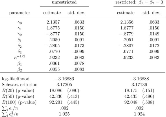
unrestricted restricted: β1 =β2 = 0
parameter estimate std. dev. estimate std. dev.
γ0 2.1357 .0633 2.1356 .0633 γ1 1.8775 .0150 1.8777 .0150 γ2 −.8777 .0150 −.8779 .0149 δ1 .2050 .0091 .2051 .0091 δ2 −.2805 .0173 −.2807 .0172 δ3 .0770 .0099 .0771 .0099 κ−1/2 .9232 .0083 .9233 .0083 β1 .0061 .0078 β2 .0055 .0083 log-likelihood −3.16886 −3.16888 Schwarz criterion 3.17205 3.17136 B(20) (p-value) 18.086 (.080) 18.175 (.151) B(50) (p-value) 42.330 (.413) 42.435 (.496) B(100) (p-value) 92.201 (.445) 92.048 (.508) P iei/n .002 .002 P ie2i/n 1.025 1.024
Table 3: ML estimates of the logistic ACM-ARMA(1,2)-model for the direction of price changes with transaction rate and -volume
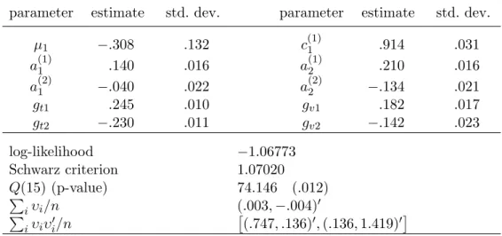
parameter estimate std. dev. parameter estimate std. dev.
µ1 −.308 .132 c(1)1 .914 .031 a(1)1 .140 .016 a(1)2 .210 .016 a(2)1 −.040 .022 a(2)2 −.134 .021 gt1 .245 .010 gv1 .182 .017 gt2 −.230 .011 gv2 −.142 .023 log-likelihood −1.06773 Schwarz criterion 1.07020 Q(15) (p-value) 74.146 (.012) P iυi/n (.003,−.004)0 P iυiυ0i/n £ (.747, .136)0,(.136,1.419)0¤
Table 4: ML estimates of the GLARMA(2,3)-model for the absolut values of the non-zero price changes with transaction rate and -volume
parameter estimate std. dev. parameter estimate std. dev.
γ0 1.409 .099 γ1 1.884 .014 γ2 −.884 .013 δ1 .199 .009 δ2 −.271 .016 δ3 .074 .009 κ−1/2 .890 .008 βt1 .122 .005 βv1 .034 .007 βt2 −.014 .005 βv2 .007 .008 log-likelihood −3.14854 Schwarz criterion 3.15244 B(20) (p-value) 17.037 (.048) B(50) (p-value) 38.376 (.498) B(100) (p-value) 84.132 (.626) P iei/n .002 P ie2i/n 1.088
B
Figures
Figure 2: Cross correlation functions of the binary variables x−1i = δi− and x1i =δ+i, indicating
the direction of price changes. The dashed lines mark off the approximative 99% confidence interval
Figure 3: Cross correlation functions of the standardized residuals υ−1i and υ1i of the
Figure 4: Auto correlation function of the non-zero absolute transaction price changes
Si|Si > 0 (left) and the standardized residuals ei of the asymmetric GLARMA(2,3)-model
(right). The dashed lines mark off the approximative 99% confidence interval±2.58/√n˜, where ˜nthe number of non-zero price changes.