Bayesian shrinkage prediction for the regression problem

(1)

www.elsevier.com/locate/jmva

Bayesian shrinkage prediction for the

regression problem

Kei Kobayashi

a,∗

, Fumiyasu Komaki

b

a_{Institute of Statistical Mathematics, Japan} b_{University of Tokyo, Japan}

Received 20 January 2007 Available online 9 February 2008

Abstract

We consider Bayesian shrinkage predictions for the Normal regression problem under the frequentist Kullback–Leibler risk function.

Firstly, we consider the multivariate Normal model with an unknown mean and a known covariance. While the unknown mean is fixed, the covariance of future samples can be different from that of training samples. We show that the Bayesian predictive distribution based on the uniform prior is dominated by that based on a class of priors if the prior distributions for the covariance and future covariance matrices are rotation invariant.

Then, we consider a class of priors for the mean parameters depending on the future covariance matrix. With such a prior, we can construct a Bayesian predictive distribution dominating that based on the uniform prior.

Lastly, applying this result to the prediction of response variables in the Normal linear regression model, we show that there exists a Bayesian predictive distribution dominating that based on the uniform prior. Minimaxity of these Bayesian predictions follows from these results.

c

AMS subject classifications:primary 62F07; 62F15; secondary 62C10; 62J07

Keywords: Bayesian prediction; Shrinkage estimation; Normal regression; Superharmonic function; Minimaxity; Kullback–Leibler divergence

1. Introduction

Suppose that we have observationsy ∼Nd(y;µ,Σ). HereNdis the density function of the

d-dimensional multivariate Normal distribution with mean vectorµand covariance matrixΣ.

∗_{Corresponding author.}

(2)

We consider the prediction ofy˜ ∼ Nd(y˜;µ,Σ˜)using a predictive density pˆ(y˜|y).We assume that the mean of the distribution of unobserved (future) samples is the same as that of the observed samples. However, the covariance matrices,ΣandΣ˜, are not necessarily the same or proportional to each other. We call a problem with such settings the “problem with changeable covariances”. As we will show below, the changeable covariance is a natural assumption when we consider the linear regression problems.

In the present work, we assume that the mean vectorµis unknown and the covariance matrix

Σ is known. We consider cases where the future covariance Σ˜ is known and ones where it is unknown.

We evaluate predictive densities pˆ(y˜|y)using the KL loss function

and the (frequentist) risk function

RKL(pˆ, θ):=

Z

p(y|θ)D(p˜(y˜|θ)k ˆp(y˜|y))dy. (2) We consider the Bayesian predictive density

p_π(y˜|y):= R ˜ p(y˜|θ)p(y|θ)π(θ)dθ R _p(y |θ)π(θ)dθ

with priorπ(θ). For the Normal model, the Bayesian predictive density with the uniform prior

πI(µ)=1 becomes p_π(y˜|y;Σ,_Σ˜₎₌ 1 (2π)d/2_|_Σ_{+ ˜}_Σ_|1/2exp − (y˜−y)>(Σ+ ˜Σ)−1(y˜−y) 2 ! ,

as we will see in Section2. Letp_π(y˜|y)denotep_π(y˜|y;Σ,Σ˜)for short.

When Σ˜ is proportional to Σ, i.e. Σ˜ = aΣ for a > 0, the problem is reduced to that withΣ = vId andΣ˜ = ˜vId for positive scalar valuesv andv˜. This case with ‘unchangeable covariances’ has been well studied. The Bayesian predictive density

pI(y˜|y;Σ,Σ˜)= 1 {2π(v+ ˜v)}d/2exp −k ˜y−yk 2 2(v+ ˜v)

based on the uniform priorπI(µ)=1 dominates the plug-in density

p(y˜| ˆµ)= 1 {2πv˜}d/2exp −k ˜y−yk 2 2v˜

with MLE, whereµˆ = y. Moreover, by [12,13], the Bayesian predictive density pI(y˜|y)is the best predictive density that is invariant under the translation group. In [11,3], the minimaxity of

pIwas proved.

In [8], it was proved that the Bayesian predictive densitypS(y˜|y)with Stein prior

πS(µ):= kµk−(d−2) (3)

(3)

George et al. [3] generalized the result of Komaki [8]. Define the marginal distributionm_π by

m_π(z;Σ):=

Z

N(z;µ,Σ)π(µ)dµ. (4)

As we will see in Theorem 2.4, George et al. [3] proved a sufficient condition on the prior

π(µ)or the marginal distributionm_π for p_π(y˜|y)to dominatepI(y˜|y)whenΣis proportional to Σ˜. In the present work, we generalize the results of Komaki and George et al. [8,3] to the corresponding problem with changeable covariances, considering only finite sample cases. Asymptotic properties of Bayesian prediction are studied in [7,1,9].

2. Prior distributions independent of the future covariance

In this section, we develop and prove our main results concerning properties of p_π(y˜|y)in the problem with changeable covariances.

First we give three lemmas generalizing results proved in [3] for the problem with “unchangeable” variances.

Define the marginal distributionm_π by(4). Here, we assume thatΣ˜ is nonsingular, though this assumption can be removed as we will see at the end of Section2.

Lemma 2.1. If m_π(z;Σ) <∞for all z, then p_π(y˜|y)is a proper probability density. Moreover, the mean of p_π(y˜|y)is equal to the posterior mean E_π[µ|y]if it exists.

Let

w:=(Σ−1+ ˜Σ−1)−1(Σ−1y+ ˜Σ−1y˜)

and

Σ_w :=(Σ−1+ ˜Σ−1)−1. (5)

As a function of the predictive density based on the uniform prior, the Bayesian predictive density based on a priorπ(µ)becomes as follows:

Lemma 2.2.

p_π(y˜|y)=pI(y˜|y)

m_π(w;Σ_w)

m_π(y;Σ) .

The following lemma is used for proving minimaxity ofp_π(y˜|y).

Lemma 2.3. The Bayesian predictive density pI(y˜|y)is minimax under the KL risk function

RKL(pˆ, µ).

Since the proofs ofLemmas 2.1and2.3are almost same as those of Lemmas 1 and 3 in [3], we omit them. We prove onlyLemma 2.2.

Proof of Lemma 2.2. p(y|µ,Σ)p(y˜|µ,Σ˜)= 1 (2π)d/2_|_Σ_|1/2exp −(y−µ) >_Σ−1₍_y₋_µ) 2 ₁ (2π)d/2_{| ˜}_Σ_|1/2

(4)

×exp −(y˜−µ) >_Σ˜−1₍_y_˜₋_µ) 2 ! = 1 (2π)d/2_|_Σ_|1/2 1 (2π)d/2_{| ˜}_Σ_|1/2exp −(w−µ) >_Σ−1 w (w−µ) 2 exp −y >_Σ−1_y 2 −y˜ >_Σ˜−1_y_˜ 2 ! exp (Σ −1_y_{+ ˜}_Σ−1_y_˜₎>₍_Σ−1_{+ ˜}_Σ−1₎−1₍_Σ−1_y_{+ ˜}_Σ−1_y_˜₎ 2 ! = 1 (2π)d/2_|_Σ w|1/2exp −(w−µ) >_Σ−1 w (w−µ) 2 × 1 (2π)d/2_|_Σ_{+ ˜}_Σ_|1/2exp − (y− ˜y)>(Σ+ ˜Σ)−1(y− ˜y) 2 ! . (6)

In the last equation, we use

Σ−1(Σ−1+ ˜Σ−1)−1Σ−1−Σ−1 =Σ−1(Σ−1+ ˜Σ−1)−1Σ−1−Σ−1(Σ−1+ ˜Σ−1)−1(Σ−1+ ˜Σ−1) = −Σ−1(Σ−1+ ˜Σ−1)−1Σ˜−1 = −(Σ+ ˜Σ)−1 and |Σ_w||Σ+ ˜Σ| = |Σ−1+ ˜Σ−1|−1|Σ+ ˜Σ| = |Σ|| ˜Σ|.

From(6), the predictive density with the uniform priorI(µ)=1 is given by

pI(y˜|y)= R p(y|µ,Σ)p(y˜|µ,Σ˜)dµ R p(y|µ,Σ)dµ =(2π)−d/2|Σ+ ˜Σ|−1/2exp −(y− ˜y) >₍_Σ_{+ ˜}_Σ₎−1₍_y_{− ˜}_y₎ 2 ! . Therefore p_π(y˜|y)= R p(y|µ,Σ)p(y˜|µ,Σ˜)π(µ)dµ R _p(y |µ,Σ)π(µ)dµ = pI(y˜|y) R N(w;µ,Σ_w)π(µ)dµ R N(y;µ,Σ)π(µ)dµ = pI(y˜|y) m_π(w;Σ_w) m_π(y;Σ) .

Next, the difference of the risk functions of the two priors is evaluated. Let

RKL(π, µ):= Z p(y|µ,Σ)D(p(y˜|µ,Σ˜)k p_π(y˜|y))dy φπ(µ,Σ):= Z N(z;µ,Σ)logm_π(z;Σ)dz. Then fromLemma 2.2,

(5)

Before stating the main results for the problem with changeable covariances, we review some results with a special setting, i.e., unchangeable covariances.

An extended real-valued functionπ(µ)on an open set R ⊂_Rpis said to besuperharmonic

when it satisfies the following properties:

1. −∞< π(µ)≤ ∞andπ(µ)6≡ ∞on any component of R. 2. π(µ)is lower semi-continuous onR.

3. IfGis an open subset ofRwith compact closureG¯ ⊂ R,w(µ)is a continuous function on

¯

G,w(µ)is harmonic onG, andπ(µ)≥w(µ)on∂G, thenπ(µ)≥w(µ)onG.

If π(µ) is a C2 function, then π(µ) is superharmonic on R if and only if 1π(µ) =

Pp i=1 ∂ 2 ∂µ2 iπ(µ) ≤0 onR. Theorem 2.4 ([8,3]).Assume d≥3. (i)If π(µ)is the Stein priorπS(µ),

v1> v2>0⇒φπ(µ, v1Id) < φπ(µ, v2Id) for allµ.

(ii)If π(µ)is a superharmonic function and m_π(z;vId) <∞for any z andv,

v1> v2>0⇒φπ(µ, v1Id)≤φπ(µ, v2Id) for allµ.

Furthermore, if m_π(z;vId)is also not constant for all v2 ≤ v ≤ v1, the inequality holds

strictly.

(iii)If √m_π(z;vId)is a superharmonic function for anyvand mπ(z;vId) <∞for any z

andv,

v1> v2>0⇒φπ(µ, v1Id)≤φπ(µ, v2Id) for allµ.

Furthermore, if m_π(z;vId)is also not constant for anyv2 ≤ v ≤ v1, the inequality holds

strictly.

We note that (iii) implies (ii) and (ii) implies (i). (i) was proved in [8]. (ii) and (iii) were proved in [3].

Theorem 2.5 is a generalization of (ii) of Theorem 2.4 to the problem with changeable covariances. For each priorπ(µ), definea rescaled priorwith respect to a positive definited×d

matrixΣ∗by

πΣ∗(µ):=π(Σ∗−1/2µ).

In particular, callπS;Σ∗(µ):=π_S(Σ∗−1/2µ)a rescaled Stein priorwith respect toΣ∗.

We consider Bayes risk with priorsp(Σ)andp˜(Σ˜):

RKL(π, µ)=

Z

(6)

where dΣmeans a Lebesgue measure for a vector space of all components of a matrixΣ. Define ϕπ(µ) := Z p(Σ)p˜(Σ˜)φ_π(µ,Σ)dΣdΣ˜ = Z p(Σ)p˜(Σ˜)N(z;µ,Σ)logm_π(z;Σ)dzdΣdΣ˜ (8) ϕ_πw(µ) := Z p(Σ)p˜(Σ˜)φ_π(µ,Σ_w)dΣdΣ˜ = Z p(Σ)p˜(Σ˜)N(z;µ,Σ_w)logm_π(z;Σ_w)dzdΣdΣ˜. (9) Then from(7), RKL(π, µ)−RKL(πI, µ)=ϕπ(µ)−ϕ_πw(µ). (10) We consider the case where p(Σ), p˜(Σ˜), andπ(µ) are rotation invariant. Here, a function

f(Σ)of a matrixΣ ∈ _Rd×dand a functiong(µ)of a vectorµ ∈_Rd×dare said to berotation invariantif f(Σ)= f(PΣP>)andg(µ) =g(Pµ), respectively, for every orthogonal matrix

P ∈_Rd×d.

Theorem 2.5. Let d ≥3. If p(Σ)and p˜(Σ˜)are rotation invariant functions andπis a rotation invariant superharmonic prior, then

RKL(πΣ, µ)≤RKL(πI, µ)

for anyµ. In particular, the Bayesian predictive distribution p_Σ(y| ˜y)withπ_Σ dominates that based onπIif πis also not constant.

Proof. We note thatm_π(z;Σ) < ∞for everyz ∈ _Rd and positive definite matrixΣ ∈ _Rd×d

fromLemma A.1in theAppendix.

First, we prove invariance ofϕ_π_Σ(µ)andϕw_π

Σ(µ)under rotations ofµ.

LetPbe ad×d orthogonal matrix; then

ϕπΣ(Pµ)= Z p(Σ)p(˜ Σ˜)N(z;Pµ,Σ)log Z N(z;µ0,Σ)π_Σ(µ0)dµ0dzdΣdΣ˜ = Z p(Σ)p˜(Σ˜)N(˜z;µ,P>ΣP)log Z N(z˜; ˜µ0,P>ΣP) ×π(Σ−1/2Pµ˜0)dµ˜0d˜zdΣdΣ˜ = Z p(PΣP>)p˜(Σ˜)N(˜z;µ,Σ)log Z N(z˜; ˜µ0,Σ)π(Σ−1/2µ˜0)dµ˜0dz˜dΣdΣ˜ =ϕ_π Σ(µ).

The proof of the rotation invariance ofϕ_πw_Σ(µ)is nearly the same. We define µ∗_:=_arg _max kµ0_k=k_µ_k kΣ−1/2µ0k kΣ_w−1/2µ0_k and τ := kΣ −1/2_µ∗_k kΣ_w−1/2µ∗_k. (11)

(7)

Note that 0< τ <1, becauseΣ˜ is positive definite. Moreover, kτΣ_w−1/2µ˜0k =τkΣ_w−1/2µ˜0k ≥ kΣ −1/2_µ_˜0_k kΣ_w−1/2µ˜0_k kΣ_w−1/2µ˜0k = kΣ−1/2µ˜0k for everyµ˜0.

From the rotation invariance ofφ_π_Σ,

ϕπΣ(µ)=ϕπΣ(µ ∗₎ = E_Σ_,_Σ˜ Z N(z;µ∗,Σ)log Z N(z; ˜µ,Σ)π(Σ−1/2µ)˜ dµ˜dz = E_Σ_,_Σ˜ Z N(z˜;Σ−1/2µ∗,Id)log Z N(˜z; ˜µ0,Id)π(µ˜0)dµ˜0dz˜ = E_Σ_,_Σ˜ Z N(z˜;τΣ_w−1/2µ∗,Id)log Z N(z˜; ˜µ0,Id)π(µ˜0)dµ˜0dz˜ = E_Σ_,_Σ˜ Z N(z˜;Σ_w−1/2µ∗, τ−2Id)log Z N(z˜; ˜µ0, τ−2Id)π(τµ˜0)dµ˜0dz˜ ≤ E_Σ_,_Σ˜ Z N(z˜;Σ_w−1/2µ∗,Id)log Z N(˜z; ˜µ0,Id)π(τµ˜0)dµ˜0dz˜ = E_Σ_,_Σ˜ Z N(z˜;µ∗,Σ_w)log Z N(z˜; ˜µ0,Σ_w)π(τΣ_w−1/2µ˜0)dµ˜0d˜z . (12) Here, inequality(12)is given byTheorem 2.4(ii).

Since every rotation invariant superharmonic function is radially nonincreasing,

π(τΣ_w−1/2µ˜0)≤π(Σ−1/2µ˜0).

From this inequality,

E_Σ_,_Σ˜ Z N(z˜;µ∗,Σ_w)log Z N(˜z; ˜µ0,Σ_w)π(τΣ_w−1/2µ˜0)dµ˜0dz˜ ≤E_Σ_,_Σ˜ Z N(z˜;µ∗,Σ_w)log Z N(z˜; ˜µ0,Σ_w)π(Σ−1/2µ˜0)dµ˜0dz˜ =ϕw_π Σ(µ ∗₎ =ϕw_π Σ(µ). (13)

In particular, ifπis not constant, inequality(12)holds strictly. Therefore, p_Σ dominates pI.

FromLemma 2.3,pΣ is proved to be minimax.

Corollary 2.6. Assume d ≥3. Let p(Σ)and p˜(Σ˜)be rotation invariant continuous functions. If π is a rotation invariant superharmonic prior, the Bayesian predictive density pΣ(y˜|y) is minimax underRKL.

Theorem 2.5andCorollary 2.6can be generalized to the case with asemi-positive definite future covariance matrixΣ˜. LetΣ˜ be ad-dimensional semi-positive matrix whose rank isk>0. Then there is ad×kmatrixLsatisfyingΣ˜ =L L>. Let{ai}d_i=−1kbe a set of orthogonal normalized

(8)

vectors that are orthogonal to each column vector ofL, i.e.L>ai =0 andai>aj =δi j fori,j = 1, . . . ,d−k. Define the Normal distribution with semi-positive definite covariance matrix by

Nd(y;µ,Σ˜)= 1 (2π)k/2_|_L>_L_|1/2exp − (y−µ)>Σ˜Ď(y−µ) 2 !_d₋_k Y i=1 δ(a>_i (y−µ))

whereΣ˜Ďis the Moore–Penrose pseudo-inverse ofΣ˜.

From the results of functional analysis, Nd(y;µ,Σ˜) for any semi-positive definite Σ˜ is equivalent to lim→0Nd(y;µ,Σ˜ +Id)as a functional on Schwartz functions ofy.

Using this equivalence and the bounded convergence theorem, Eq.(7) is valid for a semi-definite future covariance matrix if we defineΣ_w:=(Σ−1_{+ ˜}_ΣĎ₎−1_{. Because}_Σ˜Ď₆₌_0,_τ _defined

by(11)takes values in(0,1). Therefore,Theorem 2.5andCorollary 2.6hold for each semi-definite future covariance matrixΣ˜.

3. Prior distributions depending on the future covariance

In this section, we consider prior distributions depending on the future covariance matrix.

Theorem 3.2 below says that every Bayesian prediction with an adequately metrized prior dominates that based on the uniform prior. Although the assumption that priors can depend on the future covariance may seem strange, this assumption is natural when we consider the linear regression problem, as we will see in Section4.

First, we generalizeTheorem 2.4to the case with non-identity covariances. Letµandz be vectors inRdand letΣ ∈Rd×dbe a positive definite matrix.

LetΣ1 andΣ2be positive definite matrices such that Σ1 Σ2. An orthogonal matrixU and a diagonal matrixΛare given by a diagonalization ofΣ₁1/2Σ₂−1Σ₁1/2, i.e.Σ₁1/2Σ₂−1Σ₁1/2=

U>ΛU. Let A∗:=Σ₁1/2U>(Λ−1₋_I d)1/2.

Proposition 3.1. If πis a prior s.t.π(A∗µ)is a superharmonic function of µ, then

φπ(µ,Σ1)≥φπ(µ,Σ2) (14)

for anyµ∈_Rd. Inequality(14)becomes strict if πis not a constant function.

The following theorem is a direct result ofProposition 3.1.

Theorem 3.2. If π(A∗µ)is a superharmonic function of µ, then RKL(π, µ) ≤ RKL(πI, µ).

Furthermore, if πis not a constant function, the Bayesian predictive distribution p_πdominates that with the uniform priorπI.

Note thatπ(A∗_µ)_{can be superharmonic only if rank}₍_Σ

2−Σ1)≥3.

Proof of Proposition 3.1 and Theorem 3.2. Assume 0 ≺ Σ1 Σ2and letΣ₁1/2Σ₂−1Σ₁1/2 =

U>ΛUbe a diagonalization. Then, φπ(µ,Σ)= Z log Z π(ν) 1 (2π)d/2_|_Σ_|1/2exp −(x−ν) >_Σ−1₍_x₋_ν) 2 dν × 1 (2π)d/2_|_Σ_|1/2exp −(x−µ) >_Σ−1_(x₋_µ) 2 dx.

(9)

Letx˜ :=UΣ−1/2x,µ˜ =UΣ−1/2µ, andν˜=UΣ−1/2ν. By|Σ2|−1/2|Σ1|1/2= |Λ|1/2, φπ(µ,Σ2)= Z log Z π(Σ1/2U>ν)˜ 1 (2π)d/2_|_Λ_|1/2exp −(x˜− ˜ν) >_Λ−1₍_x_˜_{− ˜}_ν) 2 dν˜ × 1 (2π)d/2_|_Λ_|1/2exp −(x˜− ˜µ) >_Λ−1₍_x_˜_{− ˜}_µ) 2 dx˜ =φ π(Σ₁1/2U>_·₎(µ,˜ Λ −1_), ₍₁₅₎

whereπ(Σ₁1/2U>·)is a prior distribution whose density function is represented byπ(Σ₁1/2U>µ)

with a prior densityπ(µ). PuttingΣ2=Σ1, we get

φπ(µ,Σ1)=φ_π(_Σ1/2 1 U

>_·₎(µ,˜ Id), (16)

whereIdis thed-dimensional identity matrix.

We denote each diagonal component ofΛbyλi. Now 0< λi ≤1 for eachisinceΣ1Σ2. Letai(t):=1+t(λ_i−1−1)andA:=diag(ai). Then

φπ(µ,Σ2)−φπ(µ,Σ1)=φ_π(_Σ1/2 1 U >_·₎(µ,˜ Λ −1₎₋_φ π(Σ₁1/2U>_·₎(µ,˜ Id) = Z 1 t=0 d X i=1 ∂ai(t) ∂t ∂ ∂ai φ_π(_Σ1/2 1 U>·)( ˜ µ,A) ai(t) dt = Z 1 t=0 d X i=1 ∂a˜i(t) ∂t ∂ ∂a˜i φπ(A∗_·₎(µ,ˆ A˜) _˜ ai(t) dt = Z 1 t=0 d X i=1 ∂ ∂a˜i φπ(A∗_·₎(µ,ˆ A˜) _˜ ai(t) dt wherea˜i :=(λ−_i 1−1)−1aiandµˆ :=(Λ−1−Id)−1/2µ˜.

By assumption,π(A∗·)forA∗=Σ₁1/2U>(Λ−1−Id)1/2is superharmonic. Now it is sufficient to proveLemma 3.3(iii).

Lemma 3.3. (i)Σ_id₌₁_∂∂_aiN(x;µ,A)= 1

21N(x;µ,A)where1is the Laplacian with respect to

µ. (ii)R

f(x−t)dµ(t)is a superharmonic function of x if f is a superharmonic function and µis a positive measure onRd.

(iii) Pd

i=1_∂∂aiφπ(µ,A) ≤ 0 for any µ ∈ R d_{, a}

i > 0, and A = diag(ai) for each

superharmonic priorπ.

Proof of Lemma 3.3. Lemma (i) follows from direct calculation. For a proof of (ii), see Problem 1.7.16 of [10]. d X i=1 ∂ ∂ai φπ(µ,A)= d X i=1 ∂ ∂ai Z log Z π(ν)N(x;ν,A)dν N(x;µ,A)dx = Z d P i=1 ∂ ∂ai Rπ(ν)N(x;ν,A)dν R π(ν)N(x;ν,A)dν N(x;µ,A)dx

(10)

+ Z log Z π(ν)N(x;ν,A)dν d X i=1 ∂ ∂ai N(x;µ,A)dx. (17) Now, d X i=1 ∂ ∂ai Z π(ν)N(x;ν,A)dν= 1 21 Z π(ν)N(x;ν,A)dν≤0

fromLemma 3.3(i) and (ii). Thus, the first term of the right-hand side of(17)is non-positive. The second term of the right-hand side of(17)becomes

1 2 Z log Z π(ν)N(x;ν,A)dν 1N(x;µ,A)dx =1 2 Z 1log Z π(ν)N(x;ν,A)dν N(x;µ,A)dx (18)

by (i) and the self-adjoint property of the Laplacian. Since the logarithm of a superharmonic function is superharmonic (see Problem 1.7.16 of [10]),(18) is non-positive from (ii). Thus

Lemma 3.3(iii) is proved. Example 3.4. A rescaled Stein prior

πS;Σ2−Σ1(µ)= k(Σ2−Σ1)

−1/2_µ_k−(d−2)

satisfies the condition ofProposition 3.1andTheorem 3.2. This is because

k(Σ2−Σ1)−1/2µk−(d−2) =(µ>Σ −1/2 1 (Σ −1/2 1 Σ2Σ −1/2 1 −Id)−1Σ −1/2 1 µ) −(d−2)/2 =(µ>Σ₁−1/2U>(Λ−1−Id)−1UΣ −1/2 1 µ) −(d−2)/2_. Thus,πS;Σ2−Σ1(A ∗_µ)₌_π S(µ).

4. Application to the Normal linear regression problem

In this section, we apply the results in the previous section to the Normal linear regression problem.

Consider a Normal linear model

y=X>β+, (19)

∼Np(0, σ2Ip),

where the target variable y is a p-dimensional vector, X is a d × p matrix composed of the explanatory variables, σ2 > 0 is an unknown variance, and β is an unknownd-dimensional vector. When the rightmost column ofX>is the constant vector(1, . . . ,1)>, the model(19)is a model with a intercept,y=X>β+β₀+.

We suppose that a future sampley˜is generated by

˜

y= ˜X>β+ ˜, (20)

˜

∼Np˜(0,σ˜2Ip˜),

(11)

In the present work, we assume thatp ≥d andX X>is regular; however neither p˜ ≥d nor regularity ofX˜X˜>is necessary.

We consider the prediction problem for the linear regression model(19)and(20)with the KL risk function

˜

RKL(β,pˆπ,X,X˜):=

Z

p(y|X;β, σ2)D(p(y˜| ˜X;β,σ˜2)k p_π(y˜| ˜X,y,X;σ2,σ˜2))dy

and partial Bayesian risk function with priorsp(X)andp(˜ X˜):

˜

RKL(β,pˆπ):=

Z

p(X)p˜(X˜)R˜KL(β,pˆπ,X,X˜)dXdX˜. Note that we do not assume any prior forβ.

Next, the regression model is reduced to a Normal model discussed in Section 2. Let

y1:=(X X>)−1X yandy2:=y−X>(X X>)−1X y. Then 1 (2π)p/2exp −(X >_β₋_y₎>₍_X>_β₋_y₎ 2σ2 dy = 1 (2π)d/2_|_Σ_|1/2exp −(y1−β) >_Σ−1_(y 1−β) 2 g(y2;σ2)dy1dy2, where Σ:=σ2(X X>)−1 (21)

andg(y2;σ2)is a density function ofy2that is independent ofy1andβ.

Whenyis given,y1is a sufficient statistic ofβ, the maximum likelihood estimator, and the least-squares estimator ofβ. Thus, the regression model(19)is reduced to a Normal model

p(y1;β,Σ)=Nd(y1;β,Σ). (22)

Similarly, the regression model(20)for the future samples is reduced to a Normal model

˜

p(y˜1;β,Σ˜)=Nd(y˜1;β,Σ˜) (23)

with semi-positive definite covariance matrix. Herey˜1:=(X˜X˜>)ĎX˜y˜and

˜

Σ:= ˜σ2(X˜X˜>)Ď. (24)

The KL risk of the Bayesian predictive density with a priorπ(β)for the regression problem becomes ˜ RKL(pπ, β) = Z p(y|X;β, σ2)D(p(y˜| ˜X;β,σ˜2)k p_π(y˜| ˜X,y,X))dy = Z p(y|X;β, σ2) Z Nd(y˜1;β,Σ˜)g(y˜2; ˜σ2) ×log Nd(y˜1;β, ˜ Σ)g(y˜2; ˜σ2) R Nd(y˜1;β,Σ˜)g(y˜2; ˜σ2)Nd(y1;β,Σ)g(y2;σ2)π(β)dβ R Nd(y1;β,Σ)g(y2;σ2)π(β)dβ dy˜1dy˜2dy = Z Nd(y1;β,Σ)D(Nd(y˜1;β,Σ˜)kqπ(y˜1|y1))dy1 = RKL(qπ, β), (25)

(12)

where q_π(y˜1|y1):= R Nd(y˜1;β,Σ˜)Nd(y1;β,Σ)π(β)dβ R Nd(y1;β,Σ)π(β)dβ .

As a result, the prediction problem for the regression model (19) and (20) is reduced to a prediction problem (22) and (23). Using the result in Section 2, we construct a Bayesian prediction for the Normal regression problem.

DefineΣ,Σ˜, andΣ_w by (21)and(24), andΣ_w = (Σ−1+ ˜ΣĎ)−1, respectively, then the following theorem holds.

Theorem 4.1. Letπ_Σ(β)=π(Σ−1/2β). Let p(X)and p˜(X˜)be rotation invariant continuous functions.

(i) If π is a non-constant rotation invariant superharmonic function, then the Bayesian predictive density pΣ with a prior πΣ dominates pIwith the uniform prior πIunder the risk

˜

RKL.

(ii)If π is a rotation invariant superharmonic function, then p_Σ is minimax under the KL riskR˜KL.

Proof. If p(X)andp˜(X˜)are rotation invariant, then the distributions ofΣ =σ2(X X>)−1and

Σ_w=(σ−2(X X>)+ ˜σ−2(X˜X˜>))−1are also rotation invariant.

FromTheorem 2.5andCorollary 2.6, the theorem is derived directly.

The assumption of rotation invariance of p(x)and p(x˜) is sometimes not realistic. If we consider priors depending on the future explanatory variables, we can construct a Bayesian prediction dominating that with the uniform prior and, therefore, being a minimax prediction.

Define an orthogonal matrix U and a diagonal matrix Λ by a diagonalization of

Σ_w1/2Σ−1Σ_w1/2, i.e. Σ_w1/2Σ−1Σ_w1/2 = U>ΛU. Let A∗ := Σ_w1/2U>(Λ−1 − Id)1/2. Then the following theorem is a direct consequence ofTheorem 3.2.

Theorem 4.2. (i)If π(A∗β)is superharmonic w.r.t.βandπis non-constant, then the Bayesian prediction based on the priorπdominates that based on the uniform prior.

(ii) If π(A∗β) is superharmonic, then the Bayesian prediction based on the prior π is minimax.

Note thatπ(A∗β)can be superharmonic only if the number of future samples is more than 2. 5. Experimental results

We show several experimental results on the Bayesian prediction with shrinkage priors for regression problems.

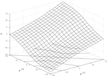
Figs. 1and2 show examples of the regression problem. We consider the five-dimensional Normal regression models, without an intercept term (Fig. 1) and with an intercept term (Fig. 2). We set the true parameterβ =(1,0, . . . ,0)∈ _R5. An explanatory variable Xis sampled from the uniform distributionU([−1,1]5×10)and a corresponding target variableyis sampled from

N10(X>β,I10). The target variable y˜ for each explanatory variable x˜ = (x˜1,0, . . . ,0)where

˜

x1∈ [0,2]is predicted by the Bayesian predictive density based on the uniform priorπIand that based on a rescaled Stein priorπS;Σ whereΣ =X X>.

Two lines inFigs. 1and2arey= ˆβ_π>x˜forπIandπS;Σ, respectively, whereβˆπis the posterior mean with priorπ. In both figures, the slope of the line with rescaled Stein prior is smaller than

(13)

Fig. 1. An example of the Bayesian prediction based on the uniform prior and a rescaled Stein prior for the Normal regression model without an intercept term.

Fig. 2. An example of the Bayesian prediction based on the uniform prior and a rescaled Stein prior for the Normal regression model with an intercept termβ0=1.

that of the one with the uniform prior because the slope parameter β is shrunk toward zero. Moreover inFig. 2, the intercept parameter is also shrunk.

Fig. 3shows the distribution functions of the predictive density pI(y˜| ˜x,y,X)withπI and

pS;Σ(y˜| ˜x,y,X)withπS;Σ, respectively, forβ = ˜x=e1:=(1,0, . . . ,0)∈R5.

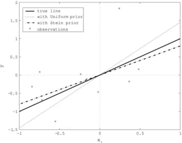
Fig. 4shows the risk functions ofpI andpΣ ford =3,5,7,9 andkβk ∈ [0,2]. The model has no intercept term. Here we assume that the columns ofX andX˜ are independently sampled fromN10(0,I10).

(14)

Fig. 3. Distribution functions ofpI(y˜| ˜x,y,X)andpS;Σ(y˜| ˜x,y,X)whereβ= ˜x =e1:=(1,0, . . . ,0)∈Rd,Xis a

sample fromU([−1,1]d×p),yis a sample fromNp(y;X>β,10Ip), andp˜(y˜| ˜x)=N(y˜; ˜x>β,10). We generate 104 samples ofy˜from each predictive distribution. The sample means ofPIandPS;Σare 1.3134 and 0.6898, respectively.

Fig. 4. The risk difference of p_I and p_S;Σ ford = 3,5,7,9 andkβk ∈ [0,2].We generate 104independent

samples of X and X˜ from N₁₀(0,I₁₀). Each line in the figure represents the sample mean of the risk difference RKL(β,pI)−RKL(β,pS;Σ). Each error bar represents the standard deviation.

Next, we show an example of Bayesian prediction whose prior depends on the explanatory variables of future samples. We set x1 = (

√ 3/2,1/2,0)>, x2 = ( √ 3/2,−1/2,0)>, x3 = (0,0,1)>,y1= √ 3/2+1/2,y2= √

3/2−1/2 andy3=0.Fig. 5is a graph ofEπS;A∗[ ˜y| ˜x,y,x] for each value ofx˜ =(x˜(1),x˜(2),0)∈ _R×_R× {0}with the rescaled Stein priorπΣ;A∗. Here,

the Bayesian estimation based on the uniform prior corresponds to the MLEβˆ =(1,1,0), i.e.

(15)

Fig. 5. An example of Bayesian prediction whose prior depends on the explanatory variables of future samples.

Fig. 6. Comparison of the risk values with five predictive densities: The Bayesian predictive densities based onp_Iand p_Σ, the ridge regression priors with regularization parametersλ=10 andλ=

√

10=3.16, and the plug-in density of the MLE. The model is five dimensional and has no intercept term. We generate 104independent samples ofXand_X˜

fromN₁₀(0,I₁₀). Each line in the figure represents the sample mean of the riskR_KL(β,pˆ)for the predictive densityp.ˆ

We can see that the amount of shrinkage with the Bayesian prediction increases as the direction of x˜ becomes closer to x(1) than x(2), i.e. x˜>e1 becomes larger than x˜>e2. This is intuitively explained as follows: When explanatory variables of training samples are closer to

x(1), x˜ whose directions are close tox(1) has more information than ones whose direction is close tox(2). Thusx˜close tox(1)need not be shrunk.

Fig. 6compares five predictive densities: The Bayesian predictive densities based onpI and

p_π_Σ, the ridge regression priors with regularization parametersλ ∈ { √

10,10}, and the plug-in density of MLE.

(16)

The ridge regression prior is πR R(β;λ)= λ d/2 (2π)d/2exp −λkβk 2 2

with a regularization parameterλ >0. We note that the posterior mean with the ridge regression prior is equivalent to the ridge regression estimator

ˆ

βR R =(X X>+λI)−1X y.

Whenkβkis close to 0, the center of shrinkage, the risk based on the ridge regression prior

πR Rbecomes smaller than that based onπΣ. However, whenkβkincreases, the prediction with πR Rbecomes worse than that withπIand even worse than the plug-in distribution of the MLE. 6. Conclusions and discussion

In this paper, we considered the multivariate Normal model with an unknown mean and a known covariance. The covariance matrix can be changed after the first sampling. We assumed rotation invariant priors of the covariance matrix and the future covariance matrix. We showed that the shrinkage predictive density with the rescaled rotation invariant superharmonic priors is minimax under the Kullback–Leibler risk. Moreover, if the prior is not constant, the Bayesian predictive density based on the prior dominates that with the uniform prior.

In this case, the rescaled priors are independent of the covariance matrix of future samples. Therefore, we can calculate the posterior distribution and the mean of the predictive distribution (i.e. the posterior mean and the Bayesian estimate for quadratic loss) based on some of the rescaled Stein priors without knowledge of future covariance. Since the predictive density with the uniform prior is minimax, that with each rescaled Stein prior is also minimax.

Next we considered Bayesian predictions whose prior can depend on the future covariance. In this case, we proved that the Bayesian prediction based on a rescaled superharmonic prior dominates that with the uniform prior without assuming the rotation invariance.

Applying these results to the prediction of response variables in the Normal regression model, we show that there exists a prior distribution such that the corresponding Bayesian predictive density dominates that based on the uniform prior. Since the prior distribution depends on the future explanatory variables, both the posterior distribution and the mean of the predictive distribution may depend on the future explanatory variables.

We note that [4] developed minimaxity and dominance conditions on prior distributions for the predictive regression problem with changeable covariance independently of our study. They also proposed a shrinkage prediction where only a subset of the regression coefficients are close to zero.

The robustness of some shrinkage methods such as the Stein estimators one has been studied (see, for example, the bibliography in [14]). The Stein effect has robustness in the sense that it depends on the loss function rather than the true distribution of the observations. Our result shows that the Stein effect has robustness with respect to the covariance of the true distribution of the future observations.

As the dimension of the model becomes large, the risk improvement with the shrinkage with the rescaled Stein priorπΣ increases as inFig. 4. An important example of a high dimensional model is that of the kernel methods (see [5]). As noted in [2], the feature space for the kernel methods is a kernel reproducing Hilbert space whose dimension is as large as the sample size.

(17)

Therefore Bayesian prediction based on shrinkage priors could be efficient for kernel methods. This is a future problem.

Acknowledgments

The authors thank Vincent Q. Vu for valuable comments on this paper. The authors would also like to thank the associate editor and two referees for their comments on and suggestions regarding an earlier version of this paper. This work was supported in part by the Ministry of Education, Science, Sports and Culture, Grant-in-Aid for JSPS Fellows, 17.10018, 2005.

Appendix. Finiteness of the marginal distribution

Here, we prove finiteness of the marginal distributionm_π(µ,Σ).

Lemma A.1. Ifπis a superharmonic prior density function, the marginal distribution m_π(x,Σ)

is finite for every vector x∈_Rdand positive definite matrixΣ ∈_Rd×d.

Proof. Fix a vector x ∈ _Rd From the definition of superharmonic functions, π 6≡ ∞. Thus,

∃x0∈Rds.t.π(x0) <∞. If we setπ(µ)˜ :=π(µ+x0), thenπ˜ is superharmonic andπ(˜ 0) <∞. Letλmaxbe the maximal eigenvalue ofΣandr0:= kx+x0k; then

m_π(x,Σ)≤ Z exp −kx+x0−µk 2 2λmax ˜ π(µ)dµ ≤ Z kµk≤2r0 exp −kx+x0−µk 2 2λmax ˜ π(µ)dµ + Z kµk>2r0 exp −kµk 2 8λmax ˜ π(µ)dµ. (26)

The first term of the right-hand side of(26)is finite because the integral of a superharmonic function over a compact subspace ofRdis finite (see Theorem 4.10 of [6]).

The second term is also finite because

∞ X n=2 Z nr0<kµk≤(n+1)r0 exp −kµk 2 8λmax ˜ π(µ)dµ≤C ∞ X n=2 exp −(nr0) 2 8λmax ˜ π(0){(n+1)r0}d for a positive constantC. Here we used the fact thatR_k_µ_k_<_rπ(µ)˜ dµ < Cπ(˜ 0)rd, by Theorem 4.9 of [6]. Therefore,m_π(x,Σ) <∞.

From this lemma, we see that the assumption m_π(z, vId) < ∞ in Theorem 2.4(ii) is redundant.

References

[1] J.M. Corcuera, F. Giummol´e, First-order optimal prediction densities, in: P. Marriott, M. Salmon (Eds.), Applications of Differential Geometry to Econometrics, Cambridge University Press, Cambridge, 2000, pp. 214–229.

[2] N. Cristianini, J. Shawe-Taylor, An Introduction to Support Vector Machines, Cambridge University Press, 2000. [3] E.I. George, F. Liang, X. Xu, Improved minimax prediction under Kullback–Leibler loss, Annals of Statistics 34

(2006) 78–91.

[4] E.I. George, X. Xu, Predictive density estimation for multiple regression, Econometric Theory 24 (2) (2008) 528–544.

(18)

[5] T. Hastie, R. Tibshirani, J. Friedman, The Elements of Statistical Learning — Data mining, Inference, and Prediction, in: Springer Series in Statistics, Springer, New York, 2001.

[6] L.L. Helms, Introduction to Potential Theory, Wiley-Interscience, New York, 1969.

[7] F. Komaki, On asymptotic properties of predictive distributions, Biometrika 83 (1996) 299–313.

[8] F. Komaki, A shrinkage predictive distribution for multivariate Normal observables, Biometrika 88 (2001) 859–864. [9] F. Komaki, Shrinkage priors for bayesian prediction, Annals of Statistics 34 (2006) 808–819.

[10] E.L. Lehmann, G. Casella, Theory of Point Estimation, 2nd ed., Springer, New York, 1998.

[11] F. Liang, A. Barron, Exact minimax strategies for predictive density estimation, data compression, and model selection, IEEE Transactions on Information Theory 50 (2004) 2708–2726.

[12] G.D. Murray, A note on the estimation of probability density functions, Biometrika 64 (1977) 150–152. [13] V.M. Ng, On the estimation of parametric density functions, Biometrika 67 (1980) 505–506.