1
Machine Learning Approaches for Traffic Flow Forecasting
By
Arsalan Ahmad Rahi
Submitted to the University of Hertfordshire in partial fulfilment of the requirement of the degree of Master of Philosophy (MPhil)
Submission Date 01/05/2019
Supervisor: DR. Sooda Ramalingam
School of Engineering and Technology University of Hertfordshire
2
DECLARATION STATEMENT
I, Arsalan Ahmad Rahi, the author of this project, hereby declare that this research study titled “Machine Learning Approach for Traffic Flow Prediction” is my own genuine work from beginning to end. I certify that the work submitted with all the materials, sources and the form of published or unpublished work of other persons used in this thesis, were duly acknowledged by means of IEEE numeric referencing. (ref. UPRAS/C/6.1, Appendix I, Section 2 – Section on cheating and plagiarism)
Student Full Name: Arsalan Ahmad Rahi
Student Registration Number: 14111965
Signed: ……… Date: 01/05/2019
3
ABSTRACT
Intelligent Transport Systems (ITS) as a field has emerged quite rapidly in the recent years. A competitive solution coupled with big data gathered for ITS applications needs the latest AI to drive the ITS for the smart and effective public transport planning and management. Although there is a strong need for ITS applications like Advanced Route Planning (ARP) and Traffic Control Systems (TCS) to take the charge and require the minimum of possible human interventions. This thesis develops the models that can predict the traffic link flows on a junction level such as road traffic flows for a freeway or highway road for all traffic conditions.
The research first reviews the state-of-the-art time series data prediction techniques with a deep focus in the field of transport Engineering along with the existing statistical and machine leaning methods and their applications for the freeway traffic flow prediction. This review setup a firm work focussed on the view point to look for the superiority in term of prediction performance of individual statistical or machine learning models over another. A detailed theoretical attention has been given, to learn the structure and working of individual chosen prediction models, in relation to the traffic flow data. In modelling the traffic flows from the real-world Highway England (HE) gathered dataset, a traffic flow objective function for highway road prediction models is proposed in a 3-stage framework including the topological breakdown of traffic network into virtual patches, further into nodes and to the basic links flow profiles behaviour estimations. The proposed objective function is tested with ten different prediction models including the statistical, shallow and deep learning constructed hybrid models for bi-directional links flow prediction methods. The effectiveness of the proposed objective function greatly enhances the accuracy of traffic flow prediction, regardless of the machine learning model used.
The proposed prediction objective function base framework gives a new approach to model the traffic network to better understand the unknown traffic flow waves and the resulting congestions caused on a junction level. In addition, the results of applied Machine Learning models indicate that RNN variant LSTMs based models in conjunction with neural networks and Deep CNNs, when applied through the proposed objective function, outperforms other chosen machine learning methods for link flow predictions. The experimentation based practical findings reveal that to arrive at an efficient, robust, offline and accurate prediction model apart from feeding the ML mode with the correct representation of the network data, attention should be paid to the deep learning model structure, data pre-processing (i.e. normalisation) and the error matrices used for data behavioural learning. The proposed framework, in future can be utilised to address one of the main aims of the smart transport systems i.e. to reduce the error rates in network wide congestion predictions and the inflicted general traffic travel time delays in real-time.
4
TABLE OF CONTENTS
DECLARATION STATEMENT ... 2 ABSTRACT ... 3 TABLE OF CONTENTS ... 4 LIST OF FIGURES ... 8 LIST OF TABLES ... 11 1. Introduction ... 12 Problem Statement ... 12Aims and Research Questions ... 13
RQ1:... 13 RQ2:... 13 RQ3:... 13 RQ4:... 13 Research Method ... 13 Contributions ... 13
What is Machine Learning? ... 14
1.5.1 How Machine Learning Works ... 14
1.5.2 Innovations in Machine Learning ... 14
1.5.3 Self-Driving Cars ... 14
1.5.4 Recommendation Systems... 14
1.5.5 Social Media Sentimental Analysis... 15
1.5.6 Online Credit Card Fraud Protection ... 15
1.5.7 Span Email Filtering ... 15
1.5.8 Network Intrusion Protection ... 15
Commonly Used Machine Learning Algorithms ... 15
1.6.1 Artificial Neural Networks ... 15
1.6.2 Decision Trees ... 16
1.6.3 Other ML Techniques ... 16
What is Smart Transportation? ... 18
1.7.1 From Commercial Transport Operators Point of View ... 18
1.7.2 Congestion as a Cause of Flow Restriction ... 19
Thesis Structure ... 19
2. Review of Traffic Flow Prediction Methods from Traditional to the State-of-the-Art Techniques 20 Introduction ... 20
5 History and Short Overview of Traffic Flow Analyses and Predictions from Literature Study 20
Study of Factors Influencing Traffic Prediction Models in the light of the Literature Review 21
2.4.1 Context of Implementation for Road Traffic Predictions ... 21
2.4.2 Input variables for Traffic Prediction ... 21
2.4.3 Effects of Using Purely Machine Learning Approaches ... 22
2.4.4 Input Data Resolution for Traffic Prediction ... 24
2.4.5 Prediction Steps in Traffic Flow Prediction ... 26
2.4.6 Seasonal Effects and Spatial-Temporal Patterns in Traffic Flow Prediction ... 27
2.4.7 Various Road Conditions in Traffic Flow Prediction ... 27
Traffic Predictions in Other Domains Closely Related to Traffic Flow ... 28
Various Approaches for Traffic Flow and Congestion Behaviour Modelling and the Associated Limitations in the Light Of Literature Review ... 31
2.6.1 Parametric, Naïve and Macroscopic Simulation based Approaches: ... 31
2.2.2 Non-Parametric and Data Driven Data Driven Machine Learning Methods: ... 32
2.6.2 Hybrid Models ... 34
Established Theoretical Relevance for the Proposed Methodology from Literature Review 35 Summary ... 36
3. Models and Architectures ... 37
Selected Models Theory ... 37
3.1.1 Historical Moving Average (HA) ... 37
3.1.2 Seasonal Autoregressive Integrated Moving Average Model (SARIMA) ... 37
3.1.3 Random Forrest Regressor (RFR) ... 38
3.1.4 Support Vector Regressor (SVR) ... 39
3.1.5 Feed Forward Backpropagation Neural Network (FFBNN) ... 40
3.1.6 Deep Belief Network (DBN) ... 41
3.1.7 Convolutional Neural Network (CNN) ... 42
3.1.8 Long Short-Term Memory (LSTM) ... 44
3.1.9 Backpropagation Long Short-Term Memory - Neural Network (B-LSTM-ANN) ... 45
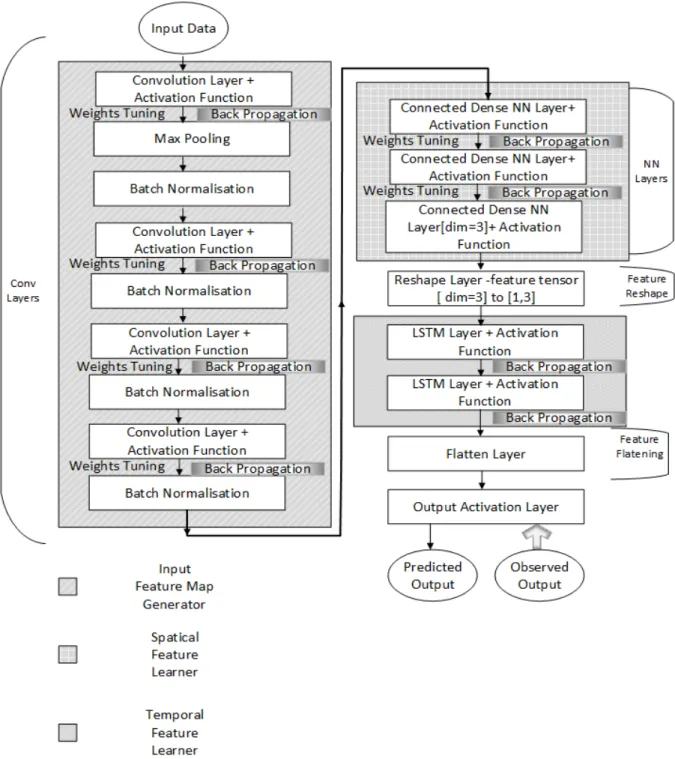
3.1.10 Deep Convolutional Neural Network - Long Short-Term Memory (DCNN-LSTM) ... 47
Hardware and Software Implementation Details ... 49
3.2.1 Data Exploration Library ... 49
3.2.1 ML Implementation Library ... 49
4. Research Methodology and Contributions ... 50
6 Study Area ... 50 Data Collection ... 50 Data Description ... 55 5.4.1 MIDAS/TAME/TMU Dataset... 55 5.4.2 AADF Dataset ... 60 Data Preparation ... 60 4.5.1 Data Cleaning ... 62 4.5.2 Data Integration ... 62 4.5.3 Data Normalisation ... 62 4.5.4 Data Reduction ... 62 4.5.5 Data Discretisation ... 62
4.5.6 Dependent and Independent Data Variables ... 62
Preliminary Analysis ... 63
4.6.1 How Network Patch and Nodes Are Defined? ... 63
4.6.2 Preparing the Dataset Subset for Each Node of a System Patch ... 64
Methodology ... 65
4.7.1 Traffic Network Representation on a Junction Level ... 66
4.7.2 Formulation of Network Flow Estimation Function ... 66
4.7.3 Node Level Traffic Flow Mathematical Representation ... 66
Summary ... 68
5. Experiments and Results: Evaluation of The Proposed Frameworks ... 69
Experimental Settings ... 69
5.1.1 Performance Metrics ... 69
5.1.2 Evaluation Settings ... 69
5.1.3 Empirical Error Distributions ... 70
5.1.4 Error Distribution Comparisons ... 70
Experiments ... 70
Case 1: Prediction Interval ... 70
Case 2: Inclusion of Related Variable ... 71
Correlation Analysis ... 71
5.3.1 Auto-Correlation ... 71
5.3.2 Cross-Correlation ... 72
5.3.3 Relation Between Traffic Flow Profiles and Times of the Day ... 74
5.3.1 Seasonality and Trends in Traffic Flows ... 77
5.3.2 Seasonality and Trends in Traffic Flows ... 78
7
Experimental Results ... 80
5.2.1 Case 1: Experiment with Different Prediction Intervals ... 80
5.2.2 Case 2: Experiment with Inclusion of the Related Variables ... 81
Summary ... 82
6. Evaluation and Conclusion ... 83
Evaluation ... 83
6.1.1 Case 1: Evaluation of Experiment Results with Different Prediction Intervals ... 83
6.1.2 Case 2: Evaluation of Experimental Results with Inclusion of the Related Variables ... 84
Discussion ... 87 6.2.1 Limitations ... 88 Conclusions ... 88 RQ1:... 88 RQ2:... 89 RQ3:... 89 RQ4:... 89 Contributions ... 90
6.4.1 Thorough ITS Literature Study on Prediction Models ... 90
6.4.2 Junction level Proposed Flow Prediction Objective Function ... 90
Future Works ... 90
References ... 91
Appendix A : Hyperparameters Tuning Results ... 97
A.1 Experiment Case1: Best Search Hyperparameters Used for Multi Prediction Horizons ... 97
Appendix B : Continuation of Discussion of Selected Models ... 114
B.1 Long Short-Term Memory (LSTM) ... 114
B.2 Traditional Neural networks (NN) VS Recurrent Neural Networks RNN: ... 114
Appendix C : Future Works ... 117
C.1 Flow Rate Network Bottleneck Identification ... 117
C.1.2 Average Congestion Speed and Average Travel Time Calculations: ... 118
C.1.3 Naïve Bayes Based Links Flow Rate Estimations: ... 119
C.1.4 Flow Rate Trend Analysis in Probability Distributions at Nodes: ... 120
C1.5 Initial Insights into Conservation of Travel Time Delays: ... 120
8
LIST OF FIGURES
Figure 1.1 Multi-Layer Perceptron (MLP) Network... 16
Figure 1.2 Supervised machine learning prediction algorithms breakdown. ... 17
Figure 1.3 Typical Wait categories as seen by the transport operators. ... 18
Figure 3. 1 RBM Structure (left) and DBN Model (right). ... 42
Figure 3. 2 Steps in Convolution Operation (left) and CNN (C-FBNN) Model (right). ... 43
Figure 3. 3 LSTM Memory Unit Structure (left) and Stacked LSTM Model (right). ... 45
Figure 3. 4 Stacked LSTM Layer Combined with NN layers (B-LSTM-ANN). ... 46
Figure 3. 5 Deep Convolutional Neural Network- Long Short-Term Memory (DCNN-LSTM) Model. .. 48
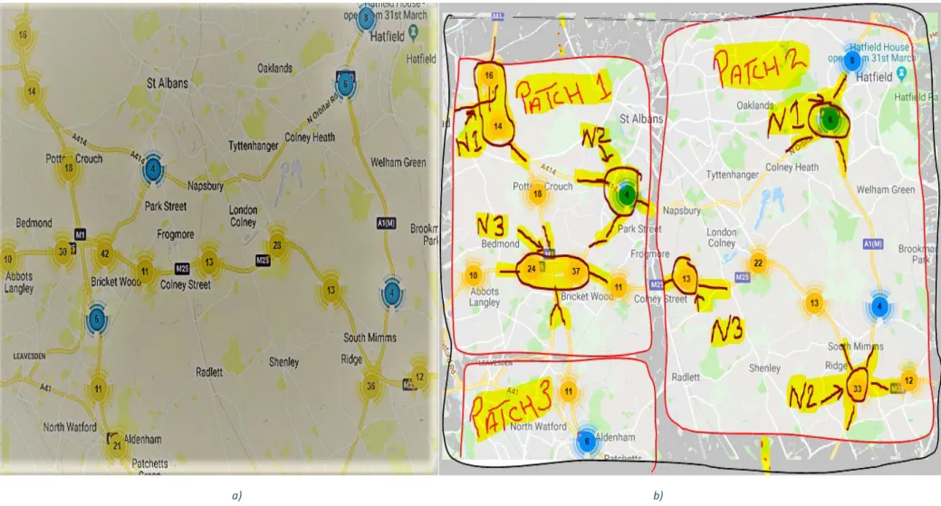
Figure 4. 1 a) Original Sample chosen test area with circles (yellow for MIDAS sites and blue for TAME sites. b) showing the sensors installed at the test sites by Highway England authority. b) Square red line boxes indicate the virtually divided network. ... 54
Figure 4. 2 Highway England Dataset Breakdown. ... 55
Figure 4. 3 DFT Dataset Breakdown. ... 60
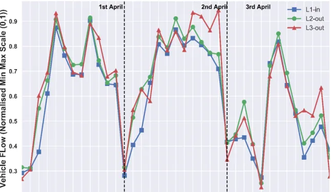
Figure 4. 4 a) First and b) last three days of pre-processed data from Patch 1, Node 2 associated Links. ... 61
Figure 4. 5 Systems as Network of Patches. ... 63
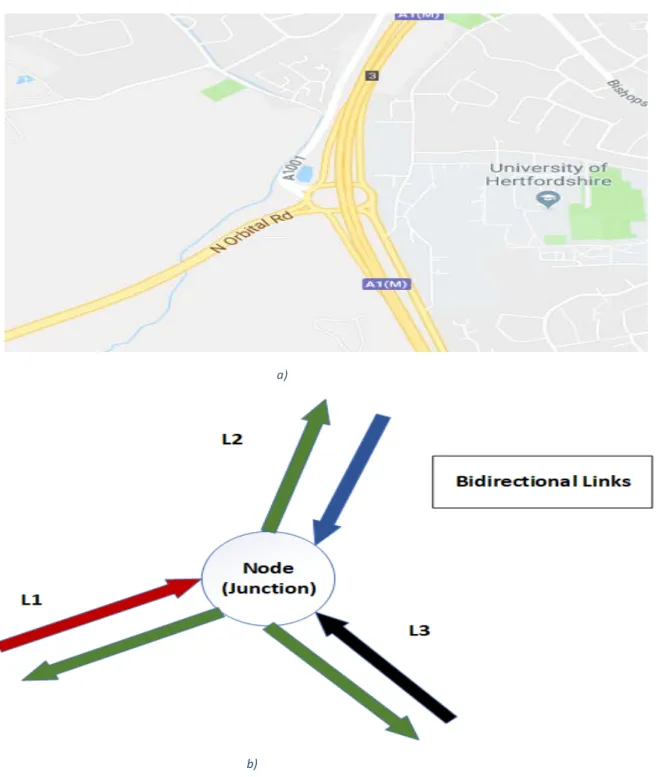
Figure 4. 6 a) 𝑃𝑃1-𝑁𝑁2, Highway junction under consideration (Google Maps, 2018). b) Node illustration retaining junction original topology. ... 64
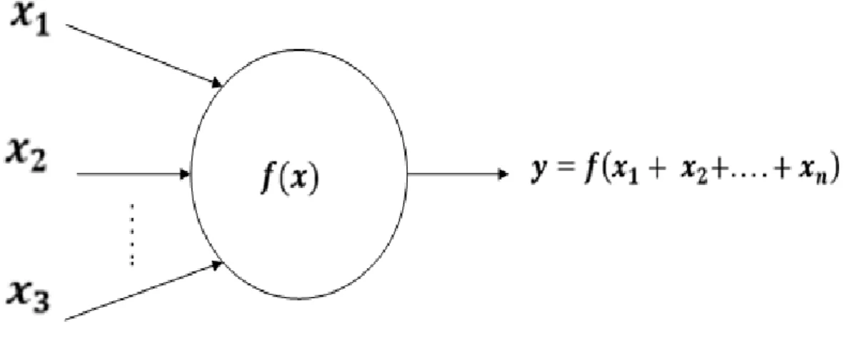
Figure 4. 7 General Network Node Link Dependencies Written in An Analogy with The General Function Definition. ... 65
Figure 4. 8 a) Extension of traffic network at node 𝑖𝑖 showing three links and their associated inflows and outflows. b) A simple traffic network at a node 𝑖𝑖 with 3 links. It shows the distribution of incoming traffic dispersed as outgoing traffic at the node. ... 67
Figure 4. 9 Implementation Steps for The Proposed Methodology. ... 68
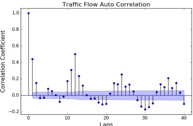
Figure 5. 1 Original Flow features auto-correlation for the incoming link 𝐿𝐿1𝑖𝑖𝑖𝑖. ... 72
Figure 5. 2 Cross Correlation of Link 𝐿𝐿1𝑖𝑖𝑖𝑖 with it's Time Lagged Versions. ... 73
Figure 5. 3 Cross-Correlation of Connected Links for The Past Six-Time Steps. ... 74
Figure 5. 4 Link 𝐿𝐿1𝑖𝑖𝑖𝑖 Normalised Flow Profiles with Respect to The Times of The Days. ... 75
Figure 5. 5 a) Correlation Between Non-Lagged Interconnected Link Pair Normalised Flows vs Time of the Day. b) Correlation Between Non-Lagged Interconnected Link Pairs Normalised Flows vs Time of the Day. ... 76
Figure 5. 6 Links Seasonality Breakdown ... 77
Figure 5. 7 Link 𝐿𝐿1𝑖𝑖𝑖𝑖 Flow Profiles with Respect to The Times of The Day Along with the Days of the Week Breakdown. ... 78
Figure 5. 8 Averaged Monthly Traffic Flows. ... 79
Figure 5. 9 Stationary Test: Augmented Dickey Fuller Test Results... 80
Figure 6. 1 Empirical CDF Plot of Absolute Mean Square Error Score on the Short-Term Prediction Results. ... 84
Figure 6. 2 Empirical CDF Plot of Absolute Mean Square Error Score on the Medium-Term Prediction Results. ... 85
9 Figure 6. 3 Empirical CDF Plot of Absolute Mean Square Error Score on the Long-Term Prediction
Results. ... 85
Figure 6. 4 Empirical CDF Plot of Absolute Mean Square Error Score on the Short-Term Prediction Results with Multi Link Proposed Flow Learning. ... 86
Figure 6. 5 Empirical CDF Plot of Absolute Mean Square Error Score on the Medium-Term Prediction Results with Multi Link Proposed Flow Learning. ... 86
Figure 6. 6 Empirical CDF Plot of Absolute Mean Square Error Score on the Long-Term Prediction Results with Multi Link Proposed Flow Learning. ... 87
Figure A.1 ARIMA Hyperparameter Grid Search for Short, Medium- and Long-Term Prediction Horizon. ... 97
Figure A.2 RFR Hyperparameter Grid Search for Short Term Prediction Horizon. ... 98
Figure A.3 RFR Hyperparameter Grid Search for Medium Term Prediction Horizon. ... 99
Figure A.4 RFR Hyperparameter Grid Search for Long Term Prediction Horizon. ... 99
Figure A.5 SVR Hyperparameter Grid Search for Short Term Prediction Horizon. ... 100
Figure A.6 SVR Hyperparameter Grid Search for Medium Term Prediction Horizon. ... 101
Figure A.7 SVR Hyperparameter Grid Search for Long Term Prediction Horizon. ... 101
Figure A.8 FFBNN Hyperparameter Grid Search, Mean Results for Short Term Prediction Horizon with Respect to Optimizers and Activation Functions. ... 102
Figure A.9 FFBNN Hyperparameter Grid Search, Mean Results for Short Term Prediction Horizon with Respect to Optimizers and Number of Epochs. ... 102
Figure A.10 FFBNN Hyperparameter Grid Search, Mean Results for Short Term Prediction Horizon with Respect to No of Neurons and Batch Sizes. ... 103
Figure A.11 FFBNN Hyperparameter Grid Search, Mean Results for Short Term Prediction Horizon with Respect to No of Neurons and Epochs. ... 103
Figure A.12 FFBNN Hyperparameter Grid Search, Mean Results for Medium Term Prediction Horizon with Respect to Optimizers and Activation Functions. ... 104
Figure A.13 FFBNN Hyperparameter Grid Search, Mean Results for Medium Term Prediction Horizon with Respect to Optimizers and Number of Epochs. ... 104
Figure A.14 FFBNN Hyperparameter Grid Search, Mean Results for Medium Term Prediction Horizon with Respect to No of Neurons and Batch Sizes. ... 105
Figure A.15 Figure FFBNN Hyperparameter Grid Search, Mean Results for Medium Term Prediction Horizon with Respect to No of Neurons and Epochs. ... 105
Figure A.16 Hyperparameter Grid Search, Mean Results for Long Term Prediction Horizon with Respect to Optimizers and Activation Functions. ... 106
Figure A.17 FFBNN Hyperparameter Grid Search, Mean Results for Long Term Prediction Horizon with Respect to Optimizers and Number of Epochs. ... 106
Figure A.18 FFBNN Hyperparameter Grid Search, Mean Results for Long Term Prediction Horizon with Respect to No of Neurons and Batch Sizes. ... 107
Figure A.19 Figure FFBNN Hyperparameter Grid Search, Mean Results for Long Term Prediction Horizon with Respect to No of Neurons and Epochs. ... 107
Figure A.20 DBN Hyperparameter Grid Search, Mean Results for Short Term Prediction Horizon with Respect to the First RBM Layer Iterations and First Layer RBMs Batch Size. ... 108
Figure A.21 DBN Hyperparameter Grid Search, Mean Results for Short Term Prediction Horizon with Respect to The Second RBM Layer Iterations and Second Layer RBMs Batch Size. ... 108
Figure A.22 DBN Hyperparameter Grid Search, Mean Results for Short Term Prediction Horizon with Respect to The Second RBM Layer Iterations and Second Layer RBMs Numbers. ... 109
10 Figure A.23 DBN Hyperparameter Grid Search, Mean Results for Short Term Prediction Horizon with Respect To The Number OF Neurons and Epochs. ... 109 Figure A.24 DBN Hyperparameter Grid Search, Mean Results for Medium Term Prediction Horizon with Respect to The First & Second RBM Layer Iterations and RBM numbers and the Model
Activation and Optimizer Functions... 110 Figure A.25 DBN Hyperparameter Grid Search, Mean Results for Medium Term Prediction Horizon with Respect To The Number OF Neurons and Second RBM Numbers. ... 110 Figure A.26 DBN Hyperparameter Grid Search, Mean Results for Medium Term Prediction Horizon with Respect to The Neural Layer Batch Size and Number of Epochs. ... 111 Figure A.27 DBN Hyperparameter Grid Search, Mean Results for Medium Term Prediction Horizon with Respect to The RBM Layer Batch Sizes. ... 111 Figure A.28 DBN Hyperparameter Grid Search, Mean Results for Long Term Prediction Horizon with Respect to The First & Second RBM Layer Iterations and RBM numbers and the Model Activation and Optimizer Functions. ... 112 Figure A.29 DBN Hyperparameter Grid Search, Mean Results for Long Term Prediction Horizon with Respect To The Number OF Neurons and Second RBM Numbers. ... 112 Figure A.30 DBN Hyperparameter Grid Search, Mean Results for Long Term Prediction Horizon with Respect to The Neural Layer Batch Size and Number of Epochs. ... 112 Figure A.31 Figure A.27 DBN Hyperparameter Grid Search, Mean Results for Long Term Prediction Horizon with Respect to The RBM Layer Batch Sizes. ... 113 Figure B.1 Data Flow and Operations in Long Short-Term Memory (LSTM) Unit Structure which Contains The Forget, Input, Output, and Update Gates. ... 114 Figure B.2 General Recurrent Neural Network Structure. Unlike a feed forward neural network each neuron not only feeds its output to the next neuron in next layer but also to the next in line neuron in the same layer. So each neuron have two sources of input, the most recent and the recent data which is combined to determine how they respond to the new data. ... 115 Figure C.1 Systematic layout of GRNGB Model. ... 117 Figure C.2 Traffic Flux versus Traffic Density generalised observation with optimum traffic flux point Q (max) differentiating the instable and stable unidirectional flow for a single link in any node [99]. ... 118 Figure C.3 Flow Rate Space-time Diagram for a single link in a node considering one direction only. ... 118
11
LIST OF TABLES
Table 2. 1 Data Resolution Used by various Prediction Models Across Literature. ... 26
Table 2. 2 Data Prediction Interval Strategy Used by various Prediction Models Across Literature. ... 27
Table 2. 3 Summary of Parametric Models. ... 32
Table 2. 4 Data Driven Models ... 33
Table 2. 5 Summary of Hybrid Models. ... 35
Table 3. 1 Layer Activation Functions. ... 40
Table 3. 2 Training Optimiser functions. ... 41
Table 4. 1 Potential Dataset Finds... 53
Table 4. 2 Traffic Flow, Additional field names and description features unique to TAME Dataset [94]. ... 58
Table 4. 3 AADF dataset common Data field names and description [93]. ... 59
Table 4. 4 Links Divisions for Patch 𝑃𝑃1(refer figure 4.1 b). ... 65
Table 5. 1 MAE and RMSE Results for The Short-Term Prediction Horizon. ... 81
Table 5. 2 MAE and RMSE Results for The Medium-Term Prediction Horizon. ... 81
Table 5. 3 MAE and RMSE Results for The Long-Term Prediction Horizon... 81
Table 5. 4 MAE and RMSE aggregated Results of The Short-Term Prediction Horizon for The Multi Feature Inclusion... 82
Table 5. 5 MAE and RMSE aggregated Results of The Medium-Term Prediction Horizon for The Multi Feature Inclusion... 82
Table 5. 6 MAE and RMSE aggregated Results of The Long-Term Prediction Horizon for The Multi Feature Inclusion... 82
12
1. Introduction
This is an introductory chapter in which the initial undertaken topic of study with a little background is presented. The subject motivation and the research questions with the aim and the contributions are also discussed.
There has been a vast increase in the big data that is available through the advent of smart things, smart cities and smart transportation and internet of things. The next thing that arose in the organisations mind is to find ways on how to put this big data in use for meaningful use. This question motivated the author to further research using the big data gathered in the field of transportation in conjunction with AI techniques to build useful systems.
Intelligent Transport Systems (ITS) is all about providing the end users the innovative and advanced services to seamlessly use different modes of transportation and traffic management for timely effective planning and to empower users to make smarter choices in the latest multi modular transportation system. Having such a system can reasonably predict the transport changes and will be of great importance for the transportation authorities, government and the public institutions. Daily we use public and private transport on our everyday commute. We take it for granted that the buses arrive on the scheduled times. Due to the ever-increasing population there is a need for the public to have the better travelling experiences on commercial transports.
Problem Statement
The issues affecting a common native may include preparing for the right currency change beforehand in terms of cash to be paid for on board ticket purchase. The bus company eventually had to pay the cost for each extra time that the passenger takes while boarding the bus. Once boarded, the passenger constantly looks out for the desired stop out of the bus window. The bus takes a certain time to reach the destination that is affected by the variable congressional regions along the route. This cycle continues day in day out. There is nothing smart about this cycle of action; this is the normal life of the bus running operations.
Public transportation has thus not evolved much enough over the past years as we expect it to along with the growing technology, so that we can call it an efficient means of operation. Technology wise, fare prices may drop, flexible dynamic congestion-based routes may be provided and ultimately bus road driving behaviour and reliability issues can be solved. Having a system that can effectively predict the traffic behaviours this will not only reduce the costs but will also help in reducing carbon footprints as well. This thesis is written to address the improvements in some of the most distinctive fields of the transportation industry that eventually constitutes to the smart transportation industry.
The closest up-to-date system deployed in the England UK today is at this website1 by Highway England. The system gives close to Realtime traffic information for most of the highways, motorways and major A roads in the England. The traffic information displayed includes the average traffic flows for each junction for clockwise and counter clockwise directions, on the corresponding motorways. The CCTV image is taken at a frequency of one minute. The data sources are the onsite deployed loop detectors and the microwave sensors at the specific locations on the road.
13 There are some of the issues inferred from the current implemented system:
o The system relies on the data collection sensors deployed at certain major road locations, which makes it easy to ascertain the traffic average road traffic speeds but at present cannot make a meaningful elaborative system so to make the sense of the nearby links.
o At the current state the system cannot make any prediction from the current data and just displays the instantly averaged speed and generates the control signals specifying the delays for the e-signs on the roads. So, there is a need of latest AI based deep machine learning techniques employment to make the effective forecasting by analysing the behaviours of the closely related traffic flow links data.
Aims and Research Questions
Based on the problem statement, the research questions explored in this research are as follows:
RQ1:
What are the potential hindering challenges for the practical implementation of the road traffic parameter forecasting systems?
RQ2:
What conventional neural network-based techniques have to offer for the traffic parameter predictions?
RQ3:
What are the state-of-the-art traffic prediction machine learning architectures for traffic flow forecasting and what effects does the proposed methodology has on the chosen model performances?
RQ4:
What deep machine learning approaches have to offer when compared to conventional or shallow machine learning techniques considering the traffic flow data?
Research Method
The background study and state of the art literature review was performed to answer the first three research questions. Proposed methodology and the null hypothesis containing the flow prediction objective function was put to test in an iterative manner for different models. The experiments were then conducted on the state-of-the-art deep ML models comparing them quantitatively with conventional ML and statistical forecasting approaches. Result based hypothesis was then drawn. The hypothesis is then further tested with multi time dependent model predictions. Conclusions are then made in the end.
Contributions
This thesis contributes by gathering the most elaborative machine learning techniques from shallow to the state-of-the-art deep learning approaches to do the predictions for traffic flows while optimising for the basic junction level highway traffic flow proposed objective function. The bi-directional flow function of individual roads is reported considering the net inflows and outflows by a
14 topological breakdown of the highway network. The proposed approach is modular and can be adopted for network wide traffic flow behavioural learning. Further the technique can help in considering the bottlenecks for congestions analysis.
What is Machine Learning?
Artificial intelligence (AI) has become one of the hot buzzwords in the recent times. Artificial Intelligence is the broader term used to describe the control algorithms and systems that derive the machines to undertake their tasks that are considered smart. Machine learning (ML) is the application of AI on machines that is since the access of relevant data to the machines will make them learn for themselves. MLs can have different types that differ in various ways but one thing which is common is that they all operate on in data. So, the data relevancy and accessibility are the main keys in any ML performance. ML is also referred to as the subset of the AI. It’s not wrong to think of ML as the current state of the art technology.
1.5.1
How Machine Learning Works
Machine learning is the set of techniques used to figure out and perform certain tasks from a given set of data. The data from a specific field that is available serves as the main driving force to the learning process of the classifier that later classifies and predicts in the future. The algorithm then devises its rules and functions either itself (unsupervised) or from users handpicked features (supervised). This phase of learning and training an algorithm is called the training phase. After this the learned algorithm instance is tested against the validation and test dataset in the training and testing phases respectively. The accuracy and performances are then categorised against standard benchmarking algorithms in a simulation environment. This approach is rather more feasible than the conventional programming approaches as humans don’t need to put a lot of effort. As more and more data become available more generalisations could be extracted from the example data. However for machine learning application to be successful one has to have a good gripping of ‘black art’ that is very hard to find in textbooks [1].
1.5.2
Innovations in Machine Learning
Machine learning is a form of analytical solution that automates the process of data analysis. Machine learning consists of algorithms that iteratively look for patterns in data and learn some useful hidden insights that can ultimately make the computer aware without programming them explicitly. Today’s machine learning has changed a lot from the machine learning of past. Now-a-days, Machine learning algorithms are being devised faster and faster due to the possibility of applying complex mathematical operations to big data that have become a reality.
1.5.3
Self-Driving Cars
Some of the widely implemented applications gaining much popularity in talks now-a-days are: The Google and tesla’s self-driving cars. They are all practically possible because of capability of the machine learning algorithms.
1.5.4
Recommendation Systems
Line of interest product recommendation systems based on ML techniques according to the customer’s buying power, taste and past order history. Purchase history drive the soul of these recommendation systems. The simplest of the price model called dynamic pricing model have been presented in [2], that predicts the possible sale purchase of the products based on the past sale data, according to the allocation of the dynamic price range group, to each individual customer and finally
15 predicting the likelihood of the products to be purchased by a particular customer. The set of products offered to the customers are selected according to their buying power or range of dynamic price group already assigned using k means-clustering technique. Finally, a binary linear-logistic regression trained classifier is called upon the test data to predict the product purchases by the potential customers.
1.5.5
Social Media Sentimental Analysis
Sentimental Analysis on the twitter tweets, a data mining and linguistic rules aggregation approach, is the form of learning algorithm that could predict the types of responses one holds towards others.
1.5.6
Online Credit Card Fraud Protection
Online Credit transaction merchandisers are currently employing machine learning techniques to detect and predict spam cases based on previous cases. This helps improve the service of these credit merchandisers and the satisfaction level of their customers.
1.5.7
Span Email Filtering
Email spam filtering is part of the classical machine learning example presented even today for the general understanding of the classification of the spam filtering from incoming emails. This helps reduce the human efforts required to check one email at a time and can safe guard the hacking prone PC’s to be safe to some extent. Simple filtering techniques use basic decision tree-based approach while complex anti-viruses may employ the traditional-hybrid algorithm combinational approach.
1.5.8 Network Intrusion Protection
Since the beginning of the wireless local area network (WLAN) era, the concerns about the general network security and intrusion have long been discussed. Now the latest machine learning approaches are being made to detect the likely causes of the different types of the network intrusions. Intrusion detection is as highly accurate as the past intrusion data provided for the learning classifier to predict it. Detection of r2I, u2r, network probes and DoS Attacks require asset of different salient feature based trained classifiers. Attack data training features can be host based features or the network based, depending upon the type and the level of intrusion attacks [3]. Recently increased interest in the machine learning in general is since the classification, data-mining and prediction phenomenon have become more popular. Things like organisational developments, big data produced by big organisations, technological advances in the computing powers, more and more advanced CPU/GPU architectures and above of all ever-getting cheaper mass data storages have sparked the researcher’s interest. This brings the researchers to get closer to use the gathered data and extract thoughtful insights from it.
Commonly Used Machine Learning Algorithms
Some of the most useful ML algorithms now-a-days, with the brief of what they are used for are listed as follows:
1.6.1
Artificial Neural Networks
A neural network (NN) is a form of popular classifier that represents the simplest human brain and mimics it’s decision making power. The artificial neural networks (ANNs) formed of combinations of perceptron’s connected in the form of different layers. Neural networks represent the complex input and output correlations that are in other ways difficult to learn and mimic in the real world. The weights assigned to each individual perceptron acts as the strengthening chain that controls the flow of the information in the form of weight values and the activation functions. Optical Electrical circuit recognition is one of the many applications of the ANN. To understand the symbols in the electrical circuit diagram, different number of ANN layers, activation functions are used to learn variety of
16 possible unique variation techniques in the training data. The test data is then utilised to measure final model performance based on its true prediction and classification power of hand drawn electrical circuit components [4]. A more general neural network architecture with deep hidden layers is shown in figure 1.1 with the generalised model equations given by equation 1.1.
Figure 1.1 Multi-Layer Perceptron (MLP) Network.
𝑦𝑦𝑡𝑡 =𝑤𝑤0+� 𝑤𝑤𝑗𝑗.𝑔𝑔(𝑤𝑤𝑖𝑖𝑗𝑗+� 𝑤𝑤0𝑗𝑗·𝑦𝑦𝑡𝑡−𝑖𝑖 𝑝𝑝 𝑗𝑗=1 ) 𝑞𝑞 𝑗𝑗=1 +𝜀𝜀𝑡𝑡 (1.1)
Given that 𝜀𝜀𝑡𝑡 is the bias term for each parameter calculations at different levels of layers.
1.6.2
Decision Trees
Decision tree is used to classify data in the classes inferred from the data itself. Dynamic Decision trees could be a more complex implementations that forms new classes or branches according to the data fed in real-time [5]. A traditional transport analysis solution could be a more fitted approach to know the decision trees in practice. In the case of transport service providers they need to form the solutions for the basic problems like: Real-time decision support, Handling incomplete data and human aware decision making powers [5]. To improve the quality of transportation planning machine learning techniques are used to read the rules from the data to provide offline planning solutions. Time consumption is a big issue in real-time planning systems by the operators. To allot the slot for the incoming request traditional optimal solutions are found to have a greater error rate in terms of the cost to avail that slot. So, an instant decision and feedback is provided to the customers by the system.
1.6.3
Other ML Techniques
Other most commonly used well established ML classification and prediction techniques include random forests (RF). Variable selection may be used for deep data interpretation, exploration and understanding. RF has shown better performance under different variable selection techniques since it reduces the correlation effect by ranking them in a special way of their importance [6].
17 Associations and sequence discovery in conjunction with other tools helps classifying the data. For an incoming data to classify it against the already existing data, it is necessary to transform the data records into ontology-based event graphs. These graphs are visual representations of event sequences through time. This mapping technique in terms of events would help in resolving data conflicts among aggregated records plotted in the form of event [7]. In an analogous manner the hybrid artificial neural network (ANN) - support vector machine (SVM) are put to use to forecast the building energy consumption with the ever growing human population [8]. Nearest-neighbour mapping, K-mean clustering, self-aware-organising maps, local optimal search techniques (genetics algorithms), expectation maximisation, Bayesian networks, principle component analysis (PCA), kernel density estimation, singular value decomposition, gaussian mixture models, sequential covering rule buildings are some of the developed ML algorithms that are often used singularly or in combination with other algorithms on a series of datasets to find the optimal solutions in terms of classifying, making predictions and fetching useful insights out of data. A breakdown of supervised techniques standardised, and basic ML techniques used in the literature previously are shown in the figure 1.2.
Figure 1.2 Supervised machine learning prediction algorithms breakdown.
Artificial Intelligence and Machine learning have become a popular subject in almost all the applied sciences in modern times. The single in hand capability of the AI and ML is its ability to generalise the behaviour of the process by and large through a large set of data gathered under various conditions, we call it Big Data. Different state of the art ML algorithms been developed over the period of the time that are considered as benchmarking standards. All newly proposed algorithms are bench marked against these standard algorithms in performance and accuracy. A dive into literature discussed in later chapters shows that ML can be developed or tuned for various parameters to
18 generalise the behaviour of data whether non-supervised or supervised and can be catered to a specific dataset or data driven application. The algorithm trained for one dataset may not be a feasible solution for the behavioural classification or prediction for another dataset.
What is Smart Transportation?
Transportation operations generate a lot of data on daily basis. Data generated by smart electronic ticket machines (ETM) and their backend servers consists of vital information from the commercial transportation providers. As deep and manual inspection is not enough, if at all, it will fail at very initial level due to the vastness of the data. There’s a high need for a detailed insight in to the raw data.
1.7.1
From Commercial Transport Operators Point of View
The raw dataset contains a useful lot of information in terms of features: Bus departure time at all stops along the route, passenger dwell time (DT) at each stop, type and number of tickets used at each stop, smart tickets vs the cash transactions, concessionary passes and then there are other indirect features that can only be discerned by manipulating the known visible features in the dataset. The raw features in the dataset that are more decisive in machine learning behaviour may not be apparent visually at all the times, and there is always a need to manipulate them in one way or the other to get the indirect features that we are interested in. Figure 1.3 shows a typical wait time division taken into consideration from a commercial transport provider’s point of view.
Figure 1.3 Typical Wait categories as seen by the transport operators.
An example of the sample smart transportation model which utilises the use of ML algorithms to model the bus deviation behaviour, let’s say, is given in its general form as:
𝐵𝐵𝐵𝐵𝐵𝐵𝐷𝐷𝐷𝐷𝐷𝐷𝑖𝑖𝐷𝐷𝐷𝐷𝑖𝑖𝐷𝐷𝑖𝑖𝑃𝑃𝑃𝑃𝐷𝐷𝑃𝑃𝑖𝑖𝑃𝑃𝐷𝐷𝑖𝑖𝐷𝐷𝑖𝑖𝑃𝑃𝑃𝑃𝐷𝐷𝑃𝑃𝐷𝐷𝐵𝐵𝐷𝐷𝑃𝑃𝐺𝐺𝐷𝐷𝑖𝑖𝐷𝐷𝑃𝑃𝐷𝐷𝐺𝐺𝑀𝑀𝐷𝐷𝑃𝑃𝐷𝐷𝐺𝐺𝑏𝑏𝐷𝐷𝐵𝐵𝐷𝐷𝑃𝑃𝑆𝑆𝐷𝐷𝐺𝐺𝐵𝐵𝐷𝐷𝑖𝑖𝐷𝐷𝑖𝑖𝐵𝐵 = 𝐴𝐴𝑃𝑃𝐷𝐷𝑖𝑖𝐴𝐴𝑖𝑖𝑃𝑃𝑖𝑖𝐷𝐷𝐺𝐺𝐼𝐼𝑖𝑖𝐷𝐷𝐷𝐷𝐺𝐺𝐺𝐺𝑖𝑖𝑔𝑔𝐷𝐷𝑖𝑖𝑃𝑃𝐷𝐷 (𝑀𝑀𝐿𝐿) + 𝑆𝑆𝐷𝐷𝐷𝐷𝐷𝐷𝑖𝑖𝐵𝐵𝐷𝐷𝑖𝑖𝑃𝑃𝐵𝐵𝑀𝑀𝐷𝐷𝑃𝑃𝐷𝐷𝐺𝐺𝐵𝐵 (1.2)
19 Equation 1.2 is the general form of the model that describes mathematically how the practical ML architecture looks like for the bus deviation predictions scenarios. Equation 1.2 consists of the terms: Artificial Intelligence (AI) techniques like smart vision, data pre-processing, Internet of thing devices and ML like Neural Networks (NN), K-mean Clustering (KC) etc... The clarification of these terms would be much clearer along the way to the algorithm development and in the final phase of the thesis implementation.
The Aim of this research work is to adapt an AI algorithm catered specifically towards the development of the transportation problem solutions that could use the existing algorithms for their better performance. Multi modular, scheduling, improved and seem-less mode of travel based on congestion and real time travel time estimations, are the tipping points to be aimed for, for the smart transportation system as for the future development.
1.7.2
Congestion as a Cause of Flow Restriction
An Intelligent transportation system consists of many smart processes that adopt a modular approach but work in harmony with each other. Understanding vehicular traffic congestion is a key for effective mobility and high-quality traffic management and safety systems. The resulting traffic congestion have counter effect on traffic flows in networks. A more empirical approach tells us that the congestion on the road happens due to a sudden breakdown. The vehicle speed decreases sharply and the vehicle density increases instead in what was initially a freeway traffic road. Subsequent research pin points the very complex spatio temporal behaviour of the traffic networks. There is a need for a traffic model to explain the empirical features of the traffic breakdown and the resulting congestion. To explain this a huge number of model and theories have already been developed. The aim of this thesis is to study and discuss the traffic flows using conventional analytical and ML techniques and to build upon them a more accurate if not efficient model, to predict the phenomenon (flows) in real congested traffic. Thus, an assessment of modelling approaches to predict the traffic breakdown is need.
Thesis Structure
Different chapters with section and subsection are devoted to building the scenario from the small problem definition to the possible questions and proposed mythology, solutions through to the state-of-the-art machine learning model architectures and concluding the thesis with the conclusions and possible future work. Rest of the chapter in the thesis are organised as follows: Chapter 2 presents the comprehensive subject review regarding the conventional statistical, machine learning and deep learning approaches for the prediction of traffic road parameter forecasting. Chapter 3 presents the state-of-the-art traffic flow prediction frameworks. Chapter presents the theoretical details of the chosen and implemented architectures using in this thesis. Research methodology is presented in chapter 5. While chapter 6 discusses the experiments, results and evaluation of the proposed frameworks quantitatively. Finally, chapter 7 concludes the thesis with the final say on the prediction model performances and provides the future direction to be built upon this thesis.
20
2.
Review of Traffic Flow Prediction Methods from Traditional to
the State-of-the-Art Techniques
Introduction
In the previous chapter a general introduction of the traffic prediction problem was discussed. A more detailed background literature study in presented in this chapter. This chapter is organised in a way that it contains the literature review discussion on traffic parameter prediction studies, with an extensive comparison breakdown of each manuscript studied comparing their adopted approach, selected features for decision making, performance measures along with adopted experimental setup using statistical or data driven machine learning (ML) based algorithmic models, sample algorithm test simulations and results as reported in the original manuscript. Further in this chapter review of applications for data prediction in the general engineering domain closely related to those of traffic engineering are also discussed. Further, based on the thorough background study an understanding of the state of the art conceptual and implemented frameworks is envisioned at the end of this chapter which highlights the key research gaps in the existing literature.
Aims
Chapter 2 presents the background detailed study on road flow and closely related traffic travel time inference models and approaches. Later, this chapter aims to synthesise the types of statistical and machine learning methods presented in the literature study. Finally, the identified gaps trigger the selection of best algorithms for our model development that are further discussed in the next chapter 3.
History and Short Overview of Traffic Flow Analyses and Predictions
from Literature Study
A survey of the recent literature suggests that many authors have contributed their well enough in the field of traffic Incident analysis, prediction and their relation in connection with the traffic congestions. A simple visualisation based approach to show traffic incidents from the past data as map overlay in the form of dynamic radial circles has been given in [9]. Traffic Origins are different coloured circles, each representing different road conditions i.e. heavy traffic, breakdowns and the congestions that are plotted on the map [9]. The traffic origins are the visual descriptors of the location of the incident, heavy traffic flow and the breakdowns whereas their radius determine the vicinity in which the traffic would be affected in one way or the other [9]. Once the area is cleared the circle recedes back and eventually vanishes at the central point of their origin [9]. According to [9], the traffic origin visualisation technique helps better in determining the effects that a cascaded accident or constricted traffic flow could potentially have on a particular road in a traffic network. From literature review traffic flows forecasting can be broadly classified into two distinct categories, Parametric approaches that are based on statistical methods for time series forecasting. Knowledge of data distributions are usually assumed in these approaches. These traffic process-based prediction methods mostly employ traffic systems simulations, road activities and driver behaviour parameters as part of the simulation process. The macroscopic traffic prediction models are based on the vehicular traffic flow analogies with fluid dynamics [10]. The major advantage of using the macroscopic simulations for traffic predictions is that in such methods traffic control parameters (e.g. delay at traffic lights, average time spent on bus stops etc.) can be used in the predictions process and the better understanding of the real traffic environment is achieved based on the locations. On the other hand, the disadvantage of
21 using much macroscopic prediction techniques are the complex parameter estimations and a real struggle to generate close to real world simulation test environment. Also, the predictions are highly influenced by the quality of the estimated traffic parameters [11]. Both the statistical ML and macroscopic approaches are useful for the ideal traffic flow prediction model development.
This research however, focuses purely on the study for the data driven statistical to complex ML methods for traffic related predictions. The major difference between the ML and conventional analytical method-based models is that ML is considered as a black box which learns the relationships between the inputs and the outputs to predict traffic variables. While ML models are complicated to optimise for the learning, but they are less complicated and computationally efficient to calculate the final prediction once trained. Continued training allows ML models to adapt to the changing behaviour displayed in the data. A detailed description of the selected models can be found in the section 4. According to the literature, for comparison to be meaningful the same traffic data needs to be used for both the statistical and computational learning models. However, such a comparison of models across the literature with same data used in different comparison scenarios is difficult to be found.
Study of Factors Influencing Traffic Prediction Models in the light of
the Literature Review
There are many factors that affect the traffic flow predictions for a model. Apart from hyperparameters of the models some of the factors are the context in which the input traffic parameters are treated, sample resolution of the input data, prediction steps, the relation between the different traffic parameters being used and the spatial based temporal dependencies hidden into the traffic variable data. Further seasonality and trend in the time series data can also influence the prediction performance. Each of these important factors are reviewed in the following subsections:
2.4.1
Context of Implementation for Road Traffic Predictions
According to the literature review traffic parameters are predicted for two main distinct types of roads that constitute the context of implementation for prediction models. One is the highway, freeway and motorways and the other being the urban road connecting roads. The major difference between the two is that urban or connecting road traffic dynamics are more difficult to understand due to uncontrolled connections and variable sized intersections. As highways form the backbone of the major long travelling road structures so the prediction models for highway predictions are majorly used for ITS applications [12]. Some examples of road predictions made in the context of highways and motorways can be found in [13][14][15][16][17][18]. The prediction models employed for the connecting and arterial roads are uncertain and structurally more complex involving more parameters and the urban networks lack the deployment of data acquisition equipment which is mostly on highway and freeways. Some examples of traffic prediction studies made in the context of urban networks can be found in [19][20][21][22][23][24][25]. One of the aims of this thesis is to find the best performing prediction model for the highway network roads.
2.4.2
Input variables for Traffic Prediction
Choice of variables may be critical and difficult for forecasting, but it is directly related to traffic flow forecasting model performance and efficiency [26]. Sometimes not just the raw feature values are used rather indirect methods of information extraction maybe employed like mutual information based on entropy theory has been used in [26]. The variable parameters that are commonly considered for the forecasting models include, traffic flow volume, travel time and speed data. Such variables data is collected with onsite sensors using loop detectors and or laser sensors. According to [27], traffic flows along with the traffic density and speed parameters are used to model complexities
22 in traffic flows in a piecewise switched linear manner, describing the model as an aggregated set of partial derivatives of the involved parameters [27].
General road delays and blocked lane duration (BLD) in [28], a queueing based model is compared considering the road delays, incident severity and road incident locations as the input parameters. For the proposed performance measure using decision trees (DT) blocked lane duration (BLD) and general road delays from a particular incident are considered in [28] as the final input parameter. Finally, the model quantifies the average delay per number of cars as the final performance parameter measure for the effective Traffic Incident Management (TIM) System. The fact that the proposed DT [28] does not require additional data makes it favourable for traffic predictions. Similarly, lane blocking incident data is used as an input parameter in automatic traffic incident detection system by considering the hybrid of Time series analysis (TSA) and machine learning (ML) techniques utilising the theory of fault diagnosis [29]. TSA is used to predict the normal traffic based upon the past normal traffic data. Likewise, ML is used to detect the traffic incidents from real-time behavioural learning, already existing normally predicted traffic data and the differences between the two [29]. The proposed approach in [29] claimed to have the better detection rate and lesser mean time for detection of incidents under the constant condition of same false alarm rate (FAR), when compared to other standard algorithms. Traffic features i.e. acceleration and other action based parameters recorded during the driving are used as input parameters and clustered together using k- mean learning in a supervised learning fashion, further tested to categorise the overall vehicle driving behaviour and later used to predict the potential traffic accidents in a driving simulation analysis [30]. Another automatic traffic incident severity classification system comparing different machine learning techniques has been presented in [31]. Input data not only contains the standard traffic incident parameters (e.g. incident location, date, time and affected lanes) but incident severity levels are also considered as an important deciding parameter to issue control commands. The proposed ML model approach in [31] is developed and tested to help manage the traffic incident management controllers to automate the network traffic control process instead of just doing them manually and breaking the information for classifying it into the pre-determined categories, and to minimize the effects an incident could have on the network [31].
2.4.3
Effects of Using Purely Machine Learning Approaches
Considering purely ML approaches, in [32], fuzzy logic–deep neural net learning (FDNN) approach have been adopted as an effort to detect the traffic road incidents, considering the traffic flow features in an urban environment. The proposed model in [32] is focussed primarily on the deep learning neural network with the aim to learn inherent spatial-temporal features from traffic flow data used an input parameter. Stacked Auto-Encoder (SAE) based layer by layer pre-training and fuzzy logic is used in conjunction with the back-propagation algorithm to control the over shoot of the learning rate and to avoid data over-fitting. Produced simulation results show an improved incident detection rate, considerably reduced false alarm rate and less learning time of FDNN compared to simple DNN [32]. Likewise, Convolutional Neural Network (CNN) based deep learning approach like in [34], with the aim to learn the spatiotemporal traffic dynamics by forming the time-space matrix images from the traffic flow data, for the network wide speed predictions, has been proposed in [35]. The results show an overall performance improvement of 42.91% with an acceptable execution time compared to the other widely used standard algorithms for predictions namely; ordinary least square method, k-nearest neighbours (KNN), artificial neural network (ANN) and long short-term memory networks neural networks (LSTM NN). The future extensions, as given by [35] could consider the possible combinations of CNN and LSTM-NN for feature learning and prediction for overall better network wide speed and flow prediction accuracy. Similar, deep learning Stacked Auto Encoder (SAE) model for the traffic data spatial temporal feature extraction and learning using a simple logistic Regressor activation
23 function based outer layer, for the network wide traffic congestion prediction is given in [36]. The SAE developed model prediction accuracy was compared with other algorithms performance accuracy which include; back propagation neural nets BP NN, random walk (RW) forecast method, support vector machines (SVM) and the radial basis function neural network (RBF-NN) [36]. An overall prediction accuracy improvement of 93% was shown by the SAE model when tested for 15 minutes average duration, traffic flow rates larger than 450 vehicles and different number of hidden layers, disregarding any other road parameters (weather, speed, density, traffic incident) had a direct or indirect effect on the traffic volumes [36]. Similarly, in [19], individual vehicular feature based behavioural study of four prominent features (speed, acceleration, and lane changing ratio) for pre-effective traffic incident detection are used in an urban environment using the mobile sensors data instead of fixed road sensors. Four different road scenarios of normal and incident traffic conditions, with having each variable passed through the Kolmogorov-Smirnov test (K-S). Final consideration of the empirical cumulative distribution function (ECDF) with an initial null-hypothesis revealed the relative importance of these variables in effectively detecting different types of traffic incidents [21]. However, [21] does suggests that for higher vehicular flow volumes (>500 veh/h) the chosen variables do not play a very significant role in differentiating between the normal and incident road conditions thus the better implementation of the incident detection system (IDS) must also consider the traffic volumes and flows.
Data Driven approach with GPS collected speed data to predict the traffic congestion evolution using spatial-temporal features learned using recurrent neural network and restricted Boltzmann machine (RNN-RBM), is given in [37]. To assist transport professional in congestion prediction and planning, [37] ruled out the common assumption that traffic flow dynamics over the networks follow the power law distribution all the times, which is generally assumed due to the lack of enough traffic sensors data. Further the proposed RNN-RBM is tested on different road networks and compared to the performance accuracy of SVM, conventional neural networks and the sensitivity analysis done with different speed thresholds, [37] reports an overall prediction of accuracy of 88%, training accuracy of 95% and finally the overall algorithm execution time to be less than 6 minutes. Further, the results are visualised on the GIS map for congested road planning. Proposed future recommended techniques includes are the model pre-training using hessian-free optimisation method for parameter rational initialisation and spatial road interaction to be considered for more precise training and prediction accuracies [37]. Support vector regressor (SVR), Bayesian classifier and linear regressor are used as main algorithms for the traffic flow estimations by predicting spatiotemporal traffic features in [38]. Traffic flow input parameter data and its relations are models into graphics form using 3D Markov random field in spatiotemporal domain. Based upon the cliques of cones obtained in the spatiotemporal domain and the overlapping between the successive cones, multiple SVR’s and Linear Regressor were used to predict the dependencies on that defined cone [38]. Finally, to predict he traffic flow for future time stamps, the speed level was found by decreasing the energy function [38]. SVR based prediction (84.64%) showed higher accuracy than the linear based approach (~76%) when tested on the test data with multiple cone zones that are not even complex geometries but also represents noisy traffic flow conditions [38].
In [39], a real-time distributed VANET approach for not just detecting the road incident-based congestion in the urban environment but also to classify congestions into different types into recurrent and non-recurrent congestions NRC (road incidents, work zones, special events and adverse weather conditions). The proposed model considers the spatial temporal causality (cause/effect features) measures with the training data produced synthetically from a real case study [39]. The algorithms tested with their prediction accuracy include: Decision tree Classifier (DT) (88.63%), Naïve Bayes (87.83%), random, Random Forest (89.51%), and boosting technique (89.17%). Future add on
24 techniques as suggested in [39] can include a voting process, a likelihood evaluation or a model to value the density of information in the data. Also, in case of real-world data with the connected vehicles strategy, Ann Arbor automated vehicle operational test can also be performed in a test environment congestion estimation. Another novel statistical approach has been discussed in [18], to detect traffic congestions from the vehicle flow/density data. The unique and advance statistics model developed in [18], uses the piecewise switched linear (PWSL) traffic model to describe the traffic flow dynamics from the data, with the leftover deterministic features from PWSL fed to exponentially weighted moving average (EWMA) chart to detect traffic congestions. EWMA performance was degraded in the presence of the real noisy data so [18] suggests the multiscale filtering before the application of EWMA.
A detailed study of literature also tells us that a fair number of researchers have given their contribution to mitigate the traffic road congestions. Reinforcement learning technique had been used to control the variable speed limits to control congestions at the recurrent freeways bottlenecks [40]. A Q-learning (QL) model in offline and variable speed limit (VSL) model in online mode has been used in conjunction with one another [40]. The VSL controller agent, which works in an online mode, is already trained with the optimal speed limits to be observed under different traffic conditions. The modified cell-based traffic model is used to evaluate the prediction-based control of trained VSL controller on a freeway recurrent bottleneck [40]. According to the paper [40], the proposed QL-VSL controller-based strategy showed a much-improved congestion optimising (travel time reduction of ~49.34% in stable conditions, ~21.89% in fluctuating traffic conditions) model than a simple feedback based VSL controller on a long-term performance basis. According to [40], the future development may include the, sophisticated prediction models, with the combination of further traffic flow estimation techniques with RL-VSM model for better performance, bottlenecks related to the incident, lane reduction, work zone, event related, merged positions of road links or even multiple bottle necks together, and other single or multiple reward functions, as part of better RL, can also be considered. Furthermore, the future recommendations in [40], are of the view to include advanced deep learning techniques as part of the VSL and overall model development strategy to improve the traffic congestions.
2.4.4
Input Data Resolution for Traffic Prediction
Input data resolution is also considered an important element for the consideration of traffic model performance. Since it can affect the quality of information to be extracted by the prediction models. According to the recent survey of traffic flow prediction mechanisms [33] the time interval or data resolution range varies from 30 seconds or one minute [34] as the least to 1 hours or 60 minutes to the most peak resolution time considered. The traffic data should be available with the data resolution that is sufficiently enough to capture the traffic dynamics by the prediction model. Along with the mentioned literature, an overview comparison of the considered time interval for the data used in the respective proposed model along with their references are presented in table 2.1. Higher recorded data resolution means more noise and less temporal resolution means the loss of data. The resolution granularity of the data should be controlled dynamically according to the prediction model. Due to the measurement instruments used for recording the traffic data it tends to be fixed in most cases and the change in traffic conditions could be missed without increasing the recorded data resolution in such a case.
25
Title & Reference Data Resolution / Time
Interval
1. On the capacity of bus transit systems [35] 1-hour recorded data resolution
2. Traffic origins: A simple visualization technique to support traffic incident analysis [9]
15-minutes recorded data resolution
3. Traffic incident data analysis and performance measures
development [28] 5-minutes aggregated data
4. A Hybrid Approach for Automatic Incident Detection [29] 1-minute data resolution 5. Traffic Flow Prediction with Big Data: A Deep Learning
Approach [36] 5-minutes aggregated data
6.
Large-scale transportation network congestion evolution prediction using deep learning theory [37]
2-minutes recorded data resolution
5, 10, 30, 60 – minutes aggregated data
7.
Predicting Spatiotemporal Traffic Flow based on Support Vector Regression and Bayesian Classifier [38]
30-seconds & 1-minute recorded data resolution 1– minutes average aggregated data 8. Effective Variables for Urban Traffic Incident Detection [19] 1-second recorded data
resolution 9. Automatic classification of traffic incident's severity using
machine learning approaches [31]
1-day recorded data resolution
10. Fuzzy Deep Learning based Urban Traffic Incident Detection
[32] 100-seconds aggregated data
11.
Learning traffic as images: A deep convolutional neural network for large-scale transportation network speed prediction [39]
1-minute recorded data resolution
2-minutes aggregated data
12. Distributed Classification of Urban Congestion Using VANET [40]
0.1-second recorded data resolution
13.
An Efficient Statistical-based Approach for Road Traffic
Congestion Monitoring [16] 1-second recorded data
resolution
14.
Reinforcement Learning-Based Variable Speed Limit Control Strategy to Reduce Traffic Congestion at Freeway Recurrent Bottlenecks [41]
30-second recorded data resolution
30-second to 5-minute aggregated data 15.
Using LSTM and GRU neural network methods for traffic flow prediction [42]
30-second recorded data resolution
5-minutes aggregated data
16.
Short-Term Traffic State Prediction Based on the Spatiotemporal Features of Critical Road Sections [43]
2-minutes recorded data resolution
2 to 15-minutes aggregated data
17.
Deep Transport: Learning Spatial-Temporal Dependency for
Traffic Condition Forecasting [44] 5-minutes recorded data
resolution
18.
Short-term traffic flow prediction using seasonal ARIMA model with limited input data [45]
1-minute recorded data resolution
10-minutes aggregated data 19.
Adaptive Kalman filter approach for stochastic short-term
traffic flow rate prediction and uncertainty quantification [46] 15-minutes aggregated data
20.
Spatiotemporal Patterns in Large-Scale Traffic Speed
26 21.
Bus Dwell Time Prediction Based on KNN [48]
---
22.
A spatiotemporal correlative k-nearest neighbor model for short-term traffic multistep forecasting [49]
5-minutes recorded data resolution
23.
A distributed spatial–temporal weighted model on
MapReduce for short-term traffic flow forecasting [50] Variable-minutes recorded data resolution
24.
Urban Traffic Flow Prediction System Using a Multifactor
Pattern Recognition Model [25] 15-minutes aggregated data
25.
Prediction of Bus Travel Time Using ANN: A Case Study in
Delhi [51] 30 to 60 minutes recorded
trip data
26.
Long short-term memory neural network for traffic speed
prediction using remote microwave sensor data [52] 2-minutes aggregated data Table 2. 1 Data Resolution Used by various Prediction Models Across Literature.
2.4.5
Prediction Steps in Traffic Flow Prediction
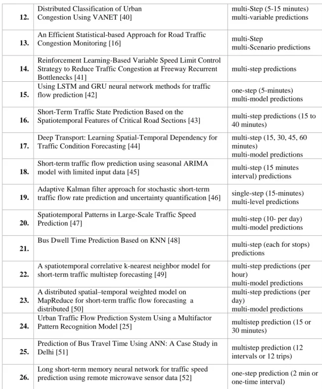
The future time steps or intervals across which the prediction model predicts is referred to as the prediction step or prediction interval or prediction horizon. A generally accepted rule is that the prediction accuracy degrades with an increase in prediction horizon [47]. Although multi-step predictions are so common in the prediction model discussed across literature, but it comes with the prediction model accuracy compromise. In this research the intension is to do both one step and multi-step ahead predictions. An overview comparison of the considered prediction multi-steps for the respective proposed model along with their references are pin table 2.2
Title & Reference Prediction Types
1. On the capacity of bus transit systems [35] multistep predictions 2. Traffic origins: A simple visualization technique to support
traffic incident analysis [9] multistep predictions
3. Traffic incident data analysis and performance measures
development [28] multistep predictions
4. A Hybrid Approach for Automatic Incident Detection [29] multistep predictions 5. Traffic Flow Prediction with Big Data: A Deep Learning
Approach [36]
multistep predictions (15, 30, 45, 60 minutes) 6. Large-scale transportation network congestion evolution
prediction using deep learning theory [37]
multistep predictions (4 -per day)
7. Predicting Spatiotemporal Traffic Flow based on
Support Vector Regression and Bayesian Classifier [38] multi-predictions model 8. Effective Variables for Urban Traffic Incident Detection [19] multi-Step Multi-variable
predictions 9. Automatic classification of traffic incident's severity using
machine learning approaches [31]
one-Step Multi-variable predictions
10. Fuzzy Deep Learning based Urban Traffic Incident Detection
[32] one-Step Predictions
11.
Learning traffic as images: A deep convolutional neural network for large-scale transportation network speed prediction [39]
multi-Step Multi-variable predictions
27 12.
Distributed Classification of Urban Congestion Using VANET [40]
multi-Step (5-15 minutes) multi-variable predictions
13.
An Efficient Statistical-based Approach for Road Traffic
Congestion Monitoring [16] multi-Step
multi-Scenario predictions
14.
Reinforcement Learning-Based Variable Speed Limit Control Strategy to Reduce Traffic Congestion at Freeway Recurrent Bottlenecks [41]
multi-step predictions
15.
Using LSTM and GRU neural network methods for traffic
flow prediction [42] one-step (5-minutes)
multi-model predictions
16.
Short-Term Traffic State Prediction Based on the
Spatiotemporal Features of Critical Road Sections [43] multi-step predictions (15 to 40 minutes)
17.
Deep Transport: Learning Spatial-Temporal Dependency for Traffic Condition Forecasting [44]
multi-step (15, 30, 45, 60 minutes)
multi-model predictions 18.
Short-term traffic flow prediction using seasonal ARIMA
model with limited input data [45] multi-step (15 minutes
interval) predictions
19.
Adaptive Kalman filter approach for stochastic short-term
traffic flow rate prediction and uncertainty quantification [46] single-step (15-minutes) multi-level predictions
20.
Spatiotemporal Patterns in Large-Scale Traffic Speed
Prediction [47] multi-step (10- per day)
multi-model predictions
21.
Bus Dwell Time Prediction Based on KNN [48]
multi-step (each for stops) predictions
22.
A spatiotemporal correlative k-nearest neighbor model for short-term traffic multistep forecasting [49]
multi-step predictions (per hour)
multi-model predictions 23.
A distributed spatial–temporal weighted model on MapReduce for short-term traffic flow forecasting a distributed [50]
multi-step predictions (per day)
multi-model predictions 24.
Urban Traffic Flow Prediction System Using a Multifactor
![Table 4. 2 Traffic Flow, Additional field names and description features unique to TAME Dataset [94]](https://thumb-us.123doks.com/thumbv2/123dok_us/357334.2539331/58.1262.119.1165.389.776/table-traffic-flow-additional-description-features-unique-dataset.webp)