This is an Open Access document downloaded from ORCA, Cardiff University's institutional
repository: http://orca.cf.ac.uk/112884/
This is the author’s version of a work that was submitted to / accepted for publication.
Citation for final published version:
Cruz-Ramírez, M., Hervás-Martínez, C., Sanchez-Monedero, Javier and Gutiérrez, P.A. 2014.
Metrics to guide a multi-objective evolutionary algorithm for ordinal classification.
Neurocomputing 135 , pp. 21-31. 10.1016/j.neucom.2013.05.058 file
Publishers page: http://dx.doi.org/10.1016/j.neucom.2013.05.058
<http://dx.doi.org/10.1016/j.neucom.2013.05.058>
Please note:
Changes made as a result of publishing processes such as copy-editing, formatting and page
numbers may not be reflected in this version. For the definitive version of this publication, please
refer to the published source. You are advised to consult the publisher’s version if you wish to cite
this paper.
This version is being made available in accordance with publisher policies. See
http://orca.cf.ac.uk/policies.html for usage policies. Copyright and moral rights for publications
made available in ORCA are retained by the copyright holders.
Metrics to Guide a Multi-Objective Evolutionary Algorithm for Ordinal
Classification
M. Cruz-Ram´ırez∗, C. Herv´as-Mart´ınez, J. S´anchez-Monedero, P.A. Guti´errez
Department of Computer Science and Numerical Analysis. University of C´ordoba, Spain
Abstract
Ordinal classification or ordinal regression are classification problems in which the labels have an ordered arrangement between them. Due to this order, alternative performance evaluation metrics are need to be used in order to consider the magnitude of errors. This paper presents an study of the use of a multi-objective optimization approach in the context of ordinal classification. We contribute a study of ordinal classification performance metrics, and propose a new performance metric, the Maximum Mean Absolute Error (M MAE). M MAEconsiders per-class distribution of patterns and the magnitude of the errors, both issues being crucial for ordinal regression problems. In addition we empirically show that some of the performance metrics are competitive objectives, which justifies the use of multi-objective optimization strategies. In our case, a multi-objective evolutionary algorithm optimizes a artificial neural network ordinal model with different pairs of metrics combinations, and we conclude that the pair of the Mean Absolute Error (MAE) and the proposed M MAE is the most favorable. A study of the relationship between the metrics of this proposal is performed, and the graphical representation in the 2 dimensional space where the search of the evolutionary algorithm takes place is analyzed. The results obtained show a good classification performance, opening new lines of research in the evaluation and model selection of ordinal classifiers.
Keywords: mean absolute error, multi-objective evolutionary algorithm, ordinal measures, ordinal classification,
ordinal regression, proportional odds model
1. Introduction
Ordinal classification or ordinal regression is a su-pervised learning problem of predicting categories that have an ordered arrangement. Although classifica-tion and regression metric problems have been thor-oughly investigated in the literature, the ordinal regres-sion problems have not received as much attention as nominal (binary or multiclass) classification. For ex-ample, people can be classified by considering whether they are high, medium, or low on some attribute or in a set of categories varying from strong agreement to strong disagreement with respect to some attitude item.
∗Corresponding author at: Department of Computer Science and
Numerical Analysis, University of C´ordoba, Rabanales Campus,
Al-bert Einstein Building 3rd Floor, 14071 C´ordoba, Spain. Tel.: +34
957 218 349; Fax:+34 957 218 630.
E-mail addresses:{mcruz,chervas,jsanchezm,pagutierrez}@uco.es
∗∗This paper is a significant extension of the work “A Preliminary
Study of Ordinal Metrics to Guide a Multi-Objective Evolutionary Al-gorithm” appearing in the 11th International Conference on Intelligent Systems Design and Applications (ISDA2011).
Hodge and Treiman [1], to analyze social class identifi-cation, scored responses as follows: “Respondents iden-tifying with the lower, working, middle, upper middle, and upper class were assigned the scores 1, 2, 3, 4, and 5, respectively”. Though sequential numbers may be assigned to such categories, the numbers assigned serve only to identify the ordering of the categories. In con-trast to regression metric problems, these ranks are fi-nite types and the metric distances between the ranks are not defined, in general; in contrast to classification problems, these ranks are also different from the labels of multiple classes due to the existence of the ordering information [2].
In the previous example, it is straightforward to think that predicting classlowerwhen the real class isupper
middleshould be considered as a more severe error than
the one associated to aworkingprediction. Thereby, or-dinal classification problems should be evaluated with specific metrics. On a first consideration, various mea-sures of ordinal association and product-moment cor-relation and regression seem to rely on very different
foundations. This is, the ordinal measures are devel-oped from a) the notion of comparing pairs of cases, or b) the product-moment system, which is considered in terms of measures of individual cases.
If methodology a) is used, and there is an order-ing of the categories but the absolute distances among them are unknown, an ordinal categorical variable is ob-tained. In that respect, in order to avoid the influence of the numbers chosen to represent the classes on the performance assessment, we should only look at the or-der relation between “true” and “predicted” class num-bers. The use of Spearman’s rank correlation coeffi-cient, rS, [3] and specially Kendall’s τb [4] is a step
forward in that direction. Moreover, other coefficients are frequently used to describe association between or-dinal measures as Goodman and Kruskal’sγ [5], and Somers’sd[6].
If methodology b) (product-moment system) is used, the most common considered measures in machine learning are the Mean Absolute Error (here denoted as
MAE) [7, 8], Root Mean Square Error (RMS E) [8], and Mean Zero-One Error (MZE, more frequently known as error rate) [8], beingMZE =1−CCR, whereCCRis the Correct Classification Rate. However, these three measures are not suitable when used to evaluate the per-formance of classifiers on ordinal unbalanced datasets [7]. The first contribution of this work is a newly pro-posed metric associated to an ordinal classifier that is the highestMAEvalue fromMAEs measured indepen-dently for each class (MaximumMAEorM MAE). This metric evaluates the performance on the worst classified class. The second contribution of this work is the analy-sis of the state-of-the-art performance metrics. Finally, we empirically show that some of the metric pairs can be non-cooperative, and consequently justify the use of a multi-objective framework to address the classifier op-timization problem.
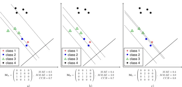
Figure 1 presents a motivational example for the present work depicting three classifiers on a fourth class ordinal classification problem. This figure illustrates how different variations of decision thresholds can af-fect to classification performance specially influenced by patterns placed on the classes boundaries. More specifically, this example raise two issues that will be studied in the current work. Firstly, using a unique performance measure may be not enough to evaluate a classifier, specially in the field of ordinal regression. Second, some of the performance metrics can result on competitive objectives on a general optimization cess since moving a threshold on a direction can pro-duce an improvement in one metric, but a detrimental on a second one.
In the present paper, the aforementioned issues are studied under a multi-objective optimization approach. Multi-objective algorithms are algorithms that optimize simultaneously objectives that are non-cooperative. In many problems there are several conflicting objectives, such as execution speed or computational cost and kind-ness of the results. For example, in [9, 10] the authors try to obtain optimal results in the shortest time and at the lowest cost. In other problems, the execution speed is not the most important and what is relevant is achiev-ing good results in different conflictachiev-ing error functions.
In the field of Artificial Neural Networks (ANNs), classification performance and model simplicity are ob-jectives that typically guide the training process of a Evolutionary Multi-Objective Algorithm (MOEA) [11], with the purpose of finding a trade-offbetween perfor-mance and model readability. Other works present the optimization of global performance versus worst clas-sified class in a Pareto based algorithm [12] or also by simplifying both objectives as a weighted linear combi-nation of the functions [13].
In ordinal classification, it is common to use several error functions when some of the classes have a number of patterns much lower than the others, i.e. ordinal im-balanced datasets. Because of this reason, we proposed
the M MAE metric measuring the performance in the
worst classified class. One real world application where this problem can be found is in the extension of donor-recipient allocation in liver transplants [14], where the classifiers aims at predicting the survival of the organ (describing this survival in three different classes, class 1: lower than 15 days, class 2: between 15 days and 3 months and, class 3: higher than 3 months). The prob-lem is that, in real cases, the number of patterns of class 1 is much lower than that of class 2 or 3. The hospi-tal would be interested in classifiers able to correctly classify all classes equally, but the bad performance for class 1 can be hidden by the fact that the number of patterns of this class is very low (for example, a good
MAEvalue can be obtained when class 1 is associated to a 5% of the patterns and the classifier never assigns a pattern to class 1). As can be seen, both objectives are conflicting (MAE and M MAE), because
improv-ing M MAEusually involves worseningMAEand vice
versa. In [15] another ordinal problem is solved from a multi-objective perspective, where six different objec-tives are considered, including MZE, MAE and four different formulations for the expected ranking accu-racy. In this work, several different ordinal measures that could be combined in the context of ordinal regres-sion are analyzed and combined in pairs for a MOEA.
class 1 class 2 class 3 class 4 class 1 class 2 class 3 class 4 class 1 class 2 class 3 class 4
Figure 1: An example of three classifiers decision boundaries for a four class ordinal classification problem. Decision thresholds vary from right to left leading to three different situations regarding performance evaluation metrics. Clas-sifiers on subfigure a) and b) have the sameCCRandM MAE, whereasMAEvaries and confusion matricesMA and
MBare different. Similar comment applies when comparing b) and c) situations, but in this caseMAEis kept constant whileCCRandM MAEvary. Finally, when comparing the classifiers a) and c), theCCRandMAE values improve and the value ofM MAEworsens.
ordinal classification performance metrics can be more suitable to guide a MOEA to obtain classifiers with a good performance (considering both the order of the miss-classification errors and the worst classified class errors). The most common ordinal classification perfor-mance metrics are reviewed, and some of them are se-lected to evaluate the performance of four nominal and ordinal classifiers, including also the proposed metric. Then, a correlation study is done between all the metrics in order to find the less correlated ones. We hypothesize that the more uncorrelated metrics are the more suit-able for acting as optimization objectives for the MOEA (given that all of them highlight positive aspects of the classifiers). The selected metrics are grouped into dif-ferent pairs that will be simultaneously optimized by the MOEA. The base classifier considered is an ANN based on the Proportional Odds Model (POM) [16] and it is evolved using a differential evolution MOEA [17, 18]. Finally, the generalization performance of the models obtained is studied with respect to the pair of metrics considered in the evolution. Because of their perfor-mance, the pairM MAE-MAEis taken special attention, deriving a relationship between this pair of metrics and studying their graphical representation.
This paper is a significant extension of a conference paper [19]. The new contributions are the following. A correlation analysis of the ordinal performance metrics is done, and the confusion matrices studied are changed
and extended. In addition, the neural network model used has been replaced by another neural network based on the Proportional Odds Model and a local search pro-cedure based on the iRprop+ algorithm [20] has been included in the MOEA to optimize the new model. Fi-nally, two additional ordinal methods have been com-pared in the experimental section, and new tables de-scribing the experiments and statistical tests have been included to enforce the conclusions.
The rest of paper is organized as follows: Section 2 shows a revision and an experimental comparison of measures for ordinal classification; Section 3 details the ordinal ANN model based on the POM model; Section 4 describes the training method employed; Section 5 de-scribes the experimental design and the results obtained, while conclusions and future research are outlined in Section 6.
2. Measures of association in ordinal classification This section presents both nominal and ordinal classi-fication performance metrics commonly used in the lit-erature. An empirical evaluation of the correlation be-tween them is done in order to select the most relevant ones.
Let’s define an ordinal classification problem as a problem where the purpose is to learn a model able to predict class labels,C = {C1,C2, . . . ,CJ}containing J
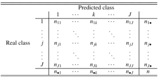
Table 1: Confusion matrix. Predicted class 1 · · · k · · · J 1 n11 · · · n1k · · · n1J n1• . . . . . . . .. . . . . .. . . . . . . Real class j nj1 · · · njk · · · njJ nj• . . . . . . . .. . . . . .. . . . . . . J nJ1 · · · nJk · · · nJ J nJ• n•1 · · · n•k · · · n•J n
labels, for unseen patterns after a training process. What makes the difference with nominal classification is that the label set has an order relationC1 ≺C2 ≺. . .≺CJ imposed on it (the symbol≺denotes the ordering be-tween different ranks). Let’s suppose an ordinal clas-sification problem with Jclasses andnpatterns with a classifiergobtaining a J×Jcontingency or confusion matrix. Table 1 shows the confusion matrix, wherenjk represents the number of times the patterns are predicted by classifiergto be in classkwhen they really belong to class j,nj•is the number of patterns belonging to class
j,n•kis the number of patterns predicted in classkand
nis the total number of patterns.
LetD ={(xi,yi), i =1,· · ·,n}be the set of training patterns, denote by{y1,y2, . . . ,yn} the set of labels of a given dataset, and let{y∗
1,y ∗ 2, . . . ,y
∗
n}be the predicted labels by the evaluated classifierg, where yi ∈ Cand
y∗
i ∈ C, andC={C1,C2, . . . ,CJ}, 1≤i≤n. In general, the predictions of the classifiers will be categories but, for some metrics, these categories will be turned into integer values by using the functionO(y∗i) which estab-lishes the position on the ordinal scale of the predicted label, beingO(Cj) = jand ifyi =Cj themO(yi) = j, 1≤ j≤J.
Many ordinal measures have been proposed to de-termine the efficiency of the classifier g, but not all pairs formed by these metrics might be valid to guide a MOEA. Before describing the ordinal metrics, accu-racy and minimum sensitivity are also presented, since they have been proved to be non-cooperative objectives [12] and they are commonly used (especially theCCR) in classification problems:
• CCR: The Correct Classification Rate or accuracy is the percentage of correctly classified patterns:
CCR= 1 n J X j=1 nj j, whereCCRvalues range from 0 to 1.
• MS: The Minimum Sensitivity is the lowest per-centage of patterns correctly predicted as
belong-ing to each class, with respect to the total number of examples in the corresponding class:
MS =min{Sj=
nj j
nj•
;j=1, ...,J},
whereSjis the sensitivity of thej-thclass andMS values range from 0 to 1.
On the other hand, there are other product-moment ordinal metrics specifically used in ordinal classifica-tion:
• MAE: The Mean Absolute Error is the average ab-solute deviation of the predicted class from the true class (i.e. average absolute deviation in number of categories of the ordinal scale) [7]:
MAE=1 n J X j,k=1 |j−k|njk= 1 n n X i=1 e(xi), wheree(xi) = |O(yi)− O(y∗
i)| is the distance be-tween the true (yi) and the predicted (y∗
i) ranks, and
O(Cj) = jis the position of a label in the ordinal rank. Then,MAEvalues range from 0 toJ−1.
• AMAE: The Average MAE is the mean of the
MAE classification errors across classes and was proposed by Baccianella et al. [7] to mitigate the effect of imbalanced class distributions. LetMAEj be theMAEfor a givenj-thclass:
MAEj= 1 nj• J X k=1 |j−k|njk= 1 nj• nj• X i=1 ej(xi),1≤ j≤J,
in such a way that:
MAE= 1 n J X j=1 nj•MAEj.
AMAEis defined in the following way:
AMAE=1 J J X j=1 MAEj,
whereAMAEvalues range from 0 toJ−1.
• M MAE: The Maximum MAE value of all the
classes is proposed in this paper as an ordinal re-gression metric alternative. M MAE is the MAE
value of the class with higher distance from the true values to the predicted ones:
whereMAEjis the MAE value for thej-thclass.
M MAEvalues range from 0 toJ−1 and it is a
nat-ural extension ofMS to ordinal regression prob-lems.
Finally association metrics are presented, which are also used in ordinal classification:
• rS: The Spearman’s rank correlation coefficient is
a non-parametric measure of statistical dependence between two variables [3]:
rS= Pn i=1(O(yi)− O(y))(O(y∗i)− O(y∗)) q Pn i=1(O(yi)− O(y))2 q Pn i=1(O(y ∗ i)− O(y ∗))2 ,
whereO(y) andO(y∗) are the average ofO(yi) and O(y∗
i),i=1, ...,n, respectively. Recall thatO(Cj)=
j.rSvalues range from -1 to 1.
• τb: The Kendall’sτis a statistic used to measure
the association between two measured quantities. Specifically, it is a measure of rank correlation [4]:
τb= Pn i,j=1c∗i jci j q Pn i,j=1c∗2i j Pn i,j=1c2i j , wherec∗i jis+1 ifO(y∗i)>O(y∗j), 0 ifO(y∗i)=O(y∗j), and -1 ifO(y∗i)<O(y∗j) fori,j=1, ...,n, and simi-lar forci j. Theτbvalues range from -1 to 1.
• W Kappa: The Weighted Kappa is a modified
ver-sion of the Kappa statistic calculated to allow as-signing different weights to different levels of ag-gregation between two variables [21]:
W Kappa= po(w)−pe(w) 1−pe(w) , where po(w)= 1 n J X j=1 J X k=1 wjknjk, and pe(w) = 1 n2 J X j=1 J X k=1 wjknj•n•k,
where the weightwjk=|j−k|quantifies the degree of discrepancy between the true (j) and the pre-dicted (k) categories, andW Kappa values range from -1 to 1.
While therSandτbmeasures are independent on the
values chosen for the ranks that represent the classes,
MAE, M MAEandAMAEdepend on the distance
be-tween ranking of two consecutive classes.
2.1. Correlations between metrics
To study the relationships between the different met-rics, a correlation matrix comparing them will be an-alyzed. This matrix is generated from the results ob-tained by four algorithms from the literature in the ten datasets used in this paper. The information about these datasets can be seen in Section 5. The experimental setup was a stratified 30-holdout in which the training set had approximately 75% of the patterns, and the gen-eralization set had the remaining ones.
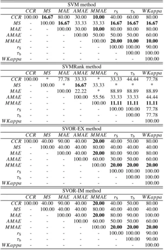
The analysis was done for each of the four meth-ods separately in order to take into account the effect of the classifier in the results (Table 2). These matri-ces were generated in the following way: firstly, since all the methods are deterministic each split of a dataset was run once for each method. So, for each method and dataset, 30 generalization models were available. The correlation between each pair of metrics through the 30 models was calculated leading to a total of 10 correlation matrices (8×8 dimensional matrices). Then, if the correlation value for a given pair of metrics was greater than 0.75, one point was summed to the corre-sponding pair. Finally, the total points of each pair was divided by the number of comparison (10) to obtain the percentage of times this pair of metrics exhibited a cor-relation higher than 0.75. When one of the two com-pared metrics (or both) was constant for the 30 models, the corresponding comparison was ignored, given that correlations could not be obtained. For example, the correlation between CCR and MS with the results of the SVM method is 16.67 due to one comparison was greater than 0.75 and four comparison could not be ob-tained (1/6=0.1667=16.67%).
This process was repeated for each method, as can be seen in Table 2. A summary of the four studies has been included in Table 3. This matrix was generated taking into account the comparison of the four methods jointly. As can be seen, the conclusions from the five matrices of both tables are very similar.
The four algorithms are widely used and have been chosen because they usually exhibit good performance. The first one, SVM, is nominal, while others are specific to ordinal regression:
• SVM: Support Vector Machines (SVM) are well known and a robust classification method. In this paper, we use the LibSVM software for the optimization of SVM [22]. This library con-tains a script for automatically adjusting the hyper-parameters associated to this kind of models, in-cluding the cost parameter and the width of the Gaussian kernels. The LibSVM grid search
cross-Table 2: Correlation matrices obtained by the different methods. Each element of each matrix is equal to the percentage of times (from a total of 10 comparison) the correlation was higher that 0.75.
SVM method
CCR MS MAE AMAE M MAE rS τb W Kappa
CCR100.00 16.67 80.00 30.00 10.00 40.00 60.00 80.00 MS - 100.00 16.67 33.33 33.33 16.67 16.67 16.67 MAE - - 100.00 30.00 10.00 80.00 80.00 80.00 AMAE - - - 100.00 50.00 50.00 50.00 60.00 M MAE - - - - 100.00 20.00 10.00 10.00 rS - - - 100.00 100.00 90.00 τb - - - 100.00 100.00 W Kappa - - - 100.00 SVMRank method
CCR MS MAE AMAE M MAE rS τb W Kappa
CCR100.00 * 77.78 33.33 * 33.33 44.44 77.78 MS - 100.00 * 16.67 33.33 * * * MAE - - 100.00 22.22 * 88.89 88.89 88.89 AMAE - - - 100.00 55.56 33.33 33.33 44.44 M MAE - - - - 100.00 11.11 11.11 11.11 rS - - - 100.00 100.00 77.78 τb - - - 100.00 77.78 W Kappa - - - 100.00 SVOR-EX method
CCR MS MAE AMAE M MAE rS τb W Kappa
CCR100.00 40.00 90.00 40.00 20.00 40.00 50.00 80.00 MS - 100.00 40.00 40.00 80.00 40.00 40.00 40.00 MAE - - 100.00 40.00 20.00 80.00 90.00 80.00 AMAE - - - 100.00 60.00 30.00 50.00 60.00 M MAE - - - - 100.00 20.00 20.00 20.00 rS - - - 100.00 100.00 100.00 τb - - - 100.00 100.00 W Kappa - - - 100.00 SVOR-IM method
CCR MS MAE AMAE M MAE rS τb W Kappa
CCR100.00 40.00 90.00 40.00 20.00 40.00 50.00 80.00 MS - 100.00 40.00 40.00 80.00 40.00 40.00 40.00 MAE - - 100.00 40.00 20.00 80.00 90.00 100.00 AMAE - - - 100.00 60.00 50.00 50.00 60.00 M MAE - - - - 100.00 20.00 20.00 20.00 rS - - - 100.00 100.00 90.00 τb - - - 100.00 90.00 W Kappa - - - 100.00
*: means that one of the two compared metrics (or both) was constant for all comparisons and, therefore, the correlation could not be obtained.
Table 3: Matrix summarizing all the correlation matri-ces of the study. Each element is equal to the percentage of times (from a total of 40 comparison) the correlation was higher that 0.75.
CCR MS MAE AMAE M MAE rS τb W Kappa
CCR100.00 22.73 84.62 35.90 12.82 38.46 51.28 79.49 MS - 100.00 22.73 31.82 54.55 22.73 22.73 22.73 MAE - - 100.00 33.33 12.82 82.05 87.18 87.18 AMAE - - - 100.00 56.41 41.03 46.15 56.41 M MAE - - - - 100.00 17.95 15.38 15.38 rS - - - 100.00 100.00 89.74 τb - - - 100.00 92.31 W Kappa - - - 100.00
validation procedure has been modified to use
MAEas the hyper-parameters selection criteria.
• SVMRank: It applies the Extended Binary Clas-sification (EBC) method [23] to SVM. The EBC method can be summarized in the following three steps. First, transform all training samples into ex-tended samples weighting these samples by using the absolute cost matrix. Second, all the extended examples are jointly learned by a binary classifier with confidence outputs, aiming at a low weighted 0/1 loss. Last step is used to convert the binary outputs to a rank.
• SVOR-EX and SVOR-IM: Support Vector
Ordi-nal Regression (SVOR) by Chu and Keerthi [24] proposes two new support vector approaches for ordinal regression. Here, multiple thresholds are optimized in order to define parallel discrimi-nant hyperplanes for the ordinal scales. The first approach includes explicit inequality constraints on the thresholds (SVOR-EX). In the second ap-proach, the samples in all the categories are al-lowed to contribute errors for each threshold, therefore there is no need of including the inequal-ity constraints in the problem. This approach is named a SVOR with implicit constraints (SVOR-IM).
According to Table 3, the pairs of measures that are less correlated (with a value lower than 20%) areCCR
-M -MAE, MAE-M MAE, M MAE-rS, M MAE-τb and
M MAE-W Kappa. Of these five pairs, the last three are very similar, because the metrics rS, τb andW Kappa
are highly correlated (values higher than 90%). There-fore, in our study will use the pair formed by M MAE
andτb. The choice ofτb is due to it is one of the most
used metrics in ordinal regression besides providing an intuitive view of the results.
Logically, the three selected pairs (CCR-M MAE,
MAE-M MAE and M MAE-τb) would be ideal
objec-tives to guide the evolution of a multi-objective algo-rithm, since they have low linear correlations and may implicitly be non-cooperative objectives. In the rest of the paper we will focus on determining which of them presents the most promising results. Note the goal of us-ing MOEA is to optimize objectives which can be non-cooperative in the solution design.
2.2. Comparison of the ordinal metrics
For the metric pairs selected, a study of their be-haviour is done by using 6 confusion matrices shown in Table 4. These matrices are designed to cover differ-ent extreme possible situations. The last two matrices represent situations where the 50 percent of patterns of
Table 5: Results obtained by the selected metrics. M1 M2 M3 M4 M5 M6 CCR 0.0 0.5 0.9 0.0 0.5 0.5 MAE 1.0 0.8 0.3 1.0 0.5 1.0 M MAE 1.0 2.0 3.0 1.0 0.5 1.0 τb 0.1972 0.8280 0.6375 0.4140 0.6669 0.1667
each class are correctly classified. The other patterns are miss-classified in adjacent classes (M5) or with a
classification error of two classes (M6). All matrices
follow the same distribution of patterns per class. The behaviour of the different metrics over other matrices can be seen in [19, 25].
Table 5 shows the results obtained after applying the selected metrics to the confusion matrices. These results show thatM1andM4have similar performance inCCR,
MAEandM MAE, but not with respect toτb. This
in-dicates thatτb is able to reflect the better performance
ofM4with respect toM1(although there the errors are
the same,M4 keeps better the relative order of the
pat-terns, given that patterns of classC1are positioned
be-fore patterns of classC2and patterns of classC3before
those of classC4). Analyzing the last two matrices is
noted that an increase in the distance of errors produces a degradation of performance ofMAE,M MAEandτb.
In addition, whenever theMAEvalues of all classes are equal,MAEandM MAEvalues are identical.
Next, the three selected metric pairs (hereafter re-ferred to as proposals) will be analyzed in order to verify the relationship between the metric of each pair:
• Proposal 1 (CCR-M MAE):M3has a good value of
CCRand a low value of M MAE. However,M1or
M4get aCCR=0, but substantially better values
ofM MAE. This indicates that these measures may
be non-cooperative.
• Proposal 2 (MAE-M MAE): M2 and M3 obtain
a very acceptable value ofMAE, while values of
MAE inM1andM4are worse. This indicates, as
in the previous case, that these metrics may be non-cooperative, because in different situations, one of them improves and the other one worsens.
• Proposal 3 (τb-M MAE): Analysing this proposal,
we see thatM2gets a great value forτb, whereas
M1 andM4 are not getting so good ones.
How-ever, M1 and M4 obtained better M MAE values
than those obtained byM2. This points out that the
measures are non-cooperative.
3. Ordinal model
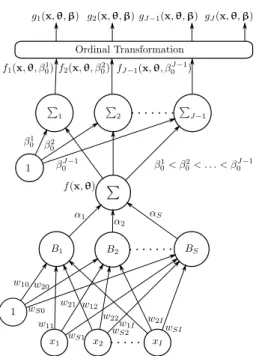
One main issue of ordinal classification is that there is no notion of the precise distance between classes. The samples are labeled by a set of ranks with different cat-egories and an order. In this paper, the classical Propor-tional Odds Model (POM) [16] adapted to ANNs [26] is considered. The POM model works based on two el-ements: the first one is a linear layer with only one node (see Figure 2) whose inputs are stamped onto a line, to give them an order which facilitates ordinal classifica-tion. After this one node linear layer, an output layer is included with one bias for each class whose objective is to classify the patterns into their corresponding class. In general, this kind of models are named to as latent variable models or threshold models [27]. The classifi-cation rule can be represented in the following general form: C(x)= C1, if f(x,θ)≤β10 C2, ifβ10< f(x,θ)≤β20 · · · CJ, if f(x,θ)> β0J−1 , (1)
where the set of biases or thresholds (β =
{β1 0, . . . , β
J−1
0 }) satisfy the following ordinal constraint:
β1 0< β
2
0<· · ·< β
J−1
0 .xis the input pattern to be
classi-fied, f(x,θ) is a ranking function andθis the vector of parameters of the model. Indeed, the analysis of Equa-tion (1) reveals the general idea previously presented: patterns,x, are projected to a real line by using the rank-ing function, f(x,θ), and the ordered biases or thresh-olds,β0j, separate the ordered classes.
Let us formally define the model for each class as
fj(x,θ, β0j)= f(x,θ)−β0j, 1≤ j≤J−1, where the pro-jection function f(x,θ) is estimated usingS sigmoidal basis functions, f(x,θ) = PS
s=1αsBs(x,ws), replacing
Bs(x,ws) by the sigmoidal equations:
Bs(x,ws)= 1
1+exp−ws0−PIi=1wsixi
whereIis the number of inputs.
By using the POM model [16], this projection can be used to obtain cumulative probabilities:
P(Y ≤ j)=P(Y =1)+· · ·+P(Y= j), 1≤j≤J−1, P(Y≤J)=1,
cumulative odds:
odds(Y≤ j)= P(Y ≤ j)
Table 4: Confusion matrices evaluated in the study. M1= 0 10 0 0 20 0 0 0 0 0 0 30 0 0 40 0 M2= 10 0 0 0 20 0 0 0 30 0 0 0 0 0 0 40 M3= 0 0 0 10 0 20 0 0 0 0 30 0 0 0 0 40 M4= 0 10 0 0 0 0 20 0 0 30 0 0 0 0 40 0 M5= 5 5 0 0 0 10 10 0 0 15 15 0 0 0 20 20 M6= 5 0 5 0 0 10 0 10 15 0 15 0 0 20 0 20
Figure 2: Neural network model for ordinal regression.
and cumulative logits:
logit(Y ≤ j)=ln P(Y ≤ j) 1−P(Y ≤ j) ! = = f(x,θ)−β0j= fj(x,θ, β0j), P(Y ≤ j)= 1 1+exp(f(x,θ)−β0j) = 1 1+exp(fj(x,θ, β0j)), where 1 ≤ j ≤ J−1, P(Y = j) is the probability a patternxhas of belonging toj-thclass,P(Y ≤ j) is the probability a patternxhas of belonging to classes 1 to j
and the logit is modeled by using the ranking function,
f(x,θ), and the corresponding bias,β0j. We can come back toP(Y= j) fromP(Y ≤ j):
P(y(nj)=1|x,θ,β)=P(Y= j)=gj(x,θ,β)= =P(Y ≤ j)−P(Y≤ j−1), j=1, . . . ,J,
wherey(nj) =1 if patternnbelongs to class jand 0 oth-erwise, and the final probability model can be expressed as: gj(x,θ,β)= 1 1+exp(fj(x,θ, β0j)) − (2) − 1 1+exp(fj−1(x,θ, βj −1 0 )) ,1≤ j≤J−1, gJ(x,θ,β)=1− 1 1+exp(fJ−1(x,θ, β0J−1)) = = exp(fJ−1(x,θ, β J−1 0 )) 1+exp(fJ−1(x,θ, β0J−1)) . 4. Method
To see how the selected metrics behave, this paper uses the MOEA described in [28]. The algorithm used is the Memetic Pareto Differential Evolution Neural Net-work (MPDENN) algorithm developed by R. Storn and K. Price in [17] and modified by H. Abbass to train neural networks [18]. MPDENN is adapted according to the trade-offbetween theCCRandMS analyzed in [12, 29]. The fundamental bases of this algorithm are Differential Evolution (DE) and the concept of Pareto dominance. DE has often been used to train neural net-works in the context of both single-objective [30, 31] and multi-objective [13, 32] optimization.
The main feature of the MPDENN algorithm is the inclusion of a crossover operator together with a muta-tion one. The crossover operator is based on the random choice of three parents, where one of them (main parent) is modified using the weighted difference of the other two (secondary parents). The child generated by the crossover and mutation operators is included in the pop-ulation if it dominates its main parent, if it has no rela-tionship with him or if it is the best child of the rejected children. A generation of the evolutionary process ends when the population has been completed. At the be-ginning of each generation, dominated individuals are eliminated from the population. The ordinal metrics are used as fitness functions of the DE algorithm without
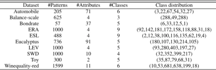
Table 6: Characteristics of the datasets.
Dataset #Patterns #Attributes #Classes Class distribution Automobile 205 71 6 (3,22,67,54,32,27) Balance-scale 625 4 3 (288,49,288) Bondrate 57 37 5 (6,33,12,5,1) ERA 1000 4 9 (92,142,181,172,158,118,88,31,18) ESL 488 4 9 (2,12,38,100,116,135,62,19,4) Eucalyptus 736 91 5 (180,107,130,214,105) LEV 1000 4 5 (93,280,403,197,27) SWD 1000 10 4 (32,352,399,217) Toy 300 2 5 (35,87,79,68,31) Winequality-red 1599 11 6 (10,53,681,638,199,18)
requiring any change in the evolutionary process. Fur-ther details can be found in [28], specially those related to the local optimization procedure included in the DE algorithm. In this paper, the improved Resilient Back-propagation (iRprop+) algorithm [20] is used as the lo-cal search procedure. Since the ordinal classification metrics are non-derivable functions, we have selected the cross-entropy error function (E) as a metric to guide the iRprop+optimization. This metric is proved to be a robust optimization metric for classification problems [33]. TheEfunction is given by:
E(θ,β)=−1 N N X n=1 J X j=1 y(nj)loggj(xn,θ,β),
wheregj(xn,θ,β) is the function defined at Equation (2). In the experiments, the local search procedure is applied every five generations.
5. Experimental study
To verify the efficiency of the three proposals, ten or-dinal datasets have been used. Nine of them are bench-mark datasets1and the other (Toy) has been generated
following the guidelines in [34]. Table 6 shows the char-acteristics of the datasets used, including the number of patterns, the number of attributes (after transform-ing nominal attributes into binary ones), the number of classes and the class distribution (number of patterns for each class).
Due to the fact that the MOEA used is non-deterministic, we perform a stratified 30-holdout, where approximately 75% of the instances are used for the training set and the remaining 25% for the test or gen-eralization set (maintaining the original distribution of classes).
1Datasets are available in http://weka.wikispaces.com/
Datasetsandhttp://mldata.org/.
The essential parameters of the algorithm (popula-tion size, number of genera(popula-tions and number of nodes in hidden layer) were obtained using a 5-fold cross-validation process on the training set. A grid search was performed using {10,25,50} for the population size,{100,150,200}for the number of generations, and
{5,10,20,30}for the number of nodes in hidden layer. The criterion to select the best parameter combination was theMAEmetric, due to it is one of the most com-monly used ordinal metrics in previous works.
5.1. Comparison methods
The results obtain by a MOEA using the three pro-posals were compared with the two following related ordinal methods.
• Proportional Odds Model (POM) [16]: this method is a cumulative link model, specifically designed for ordinal regression. This model is inspired by the latent variable motivation which provides a solid probabilistic interpretation. In this work, the POM algorithm is used with thelogitlink function, the most extended one. More details of this method have been seen in Section 3.
• Neural Network based on Proportional Odds
Model (NNPOM) [35]: this model is a non-linear version of the POM model, which combines neu-ral networks with a cumulative link model. In this method, the output of a neural network is used as latent variable for the POM model. This type of model can be optimized by maximum likelihood optimization. In this work, the model is optimized using the same local search procedure employed by the MPDENN algorithm, iRprop+. The corre-sponding parameters have been cross-validated us-ing theMAEmetric and the same ranges.
5.2. Results
Table 7 shows theCCRresults obtained after guiding the MOEA with the three proposals. They correspond
to the averages and the standard deviations of the gen-eralization results for the 30 models which are Pareto front extremes generated in 30 runs (one Pareto front for each run is obtained and then the two extremes of the front, in training, are extracted. See Figure 3 to lo-cate these models). In addition, the two ordinal methods are included for comparison. The last part of the Table 7 includes the ranking over all the datasets. The ranking is obtained in the usual manner (for each dataset, a 1 is assigned to the best method, and a 8 to worst one) [36]. Similarly, Tables 8, 9 and 10 show the results obtained for the metricsMAE,M MAEandτb, respectively.
From a descriptive point of view, forCCR, the best ranking is obtained by the proposal 2, model 1, and the second by the proposal 1, model 1 (Table 7). For
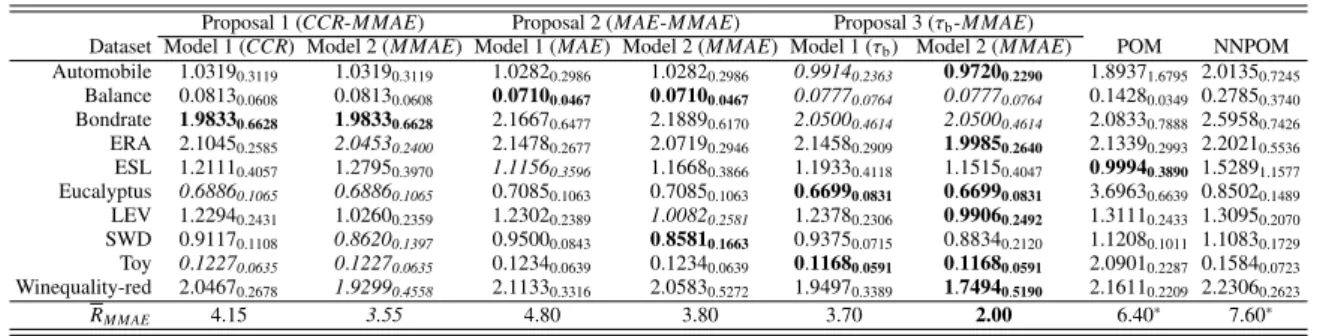
MAE(Table 8), the best rankings obtained are similar to those obtained forCCR. ForM MAE(Table 9), the best ranking is obtained by the proposal 3, model 2, and the second by the model 1 of the same proposal. Forτb
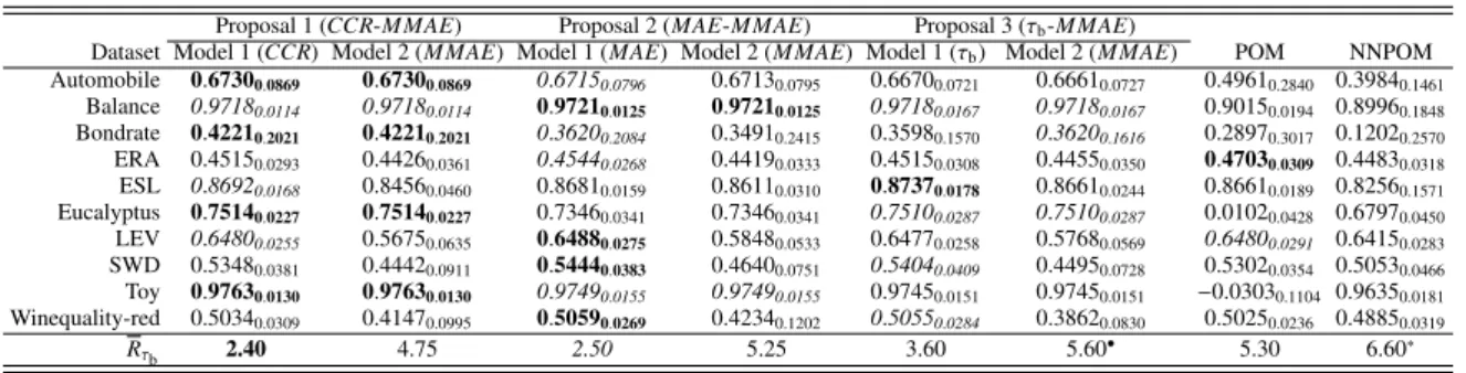
(Table 10), the best ranking is obtained by the proposal 1, model 1, and the second by the proposal 2, model 1. These results show that the best proposal is the second one (MAE-M MAEpair), because the trained classifiers has better performance on two metrics (CCRandMAE) and the second best ones onτb. It should be pointed
out that, according to the experiments,τb is not a
suit-able fitness function since the best and second best mean ranking inτbare not achieved by the proposal
optimiz-ingτb (see Table 10). In addition, the three proposals
presented competitive results compared with the refer-ence ordinal methods (POM and NNPOM).
A common feature of the three proposals is that the
M MAEmodels do not perform well for global
classifi-cation metrics (CCR,MAEandτb). The reason for this
behavior is that these models are focused on the clas-sification of the worst classified class. However, these models obtain the best results inM MAE, minimizing the maximum error across all the classes. In addition, during the evolutionary process, these models help to the opposite extreme models to improve their perfor-mance in the worst classified class because they incor-porate diversity within the individuals population.
In order to determine the statistical significance of the rank differences observed for each method in the dif-ferent datasets, a Friedman tests [37] have been carried out with a significance level ofα = 0.05. When there are significant differences, the Bonferroni-Dunn’s test is used to compare all methods to each other. This test considers that the performance of any two methods is deemed to be significantly different if their mean ranks differ by at least the critical difference (CD):
CD=q
r
K(K+1)
6D ,
whereK is the number of classifiers,Dthe number of datasets and theqvalue can be computed as suggested in [38]. We chose the best performing method (for each metric) as the control one for comparison with the rest. The ranks with significant differences forα=0.05 are marked with an∗in Tables 7, 8, 9 and 10 and forα = 0.10 with a•.
In general, the NNPOM method is the worst one with a significantly worse value for all metrics (withα=0.05
forMAE,M MAEandτbandα=0.10 forCCR), when
compared with the best method in each case. The POM method is significantly worse in M MAE andτb (both
withα =0.05) and the proposal 3-, model 2 (M MAE
extreme of the τb-M MAE pair) is worse in τb (with
α = 0.10). The greatest differences were found in the
M MAE results. The reason for these differences may
be due to the classical ordinal methods do not consider the performance for the worst classified class.
5.3. Study of the relationship between the M MAE and MAE metrics
In accordance with the results presented in the pre-vious section, a good pair for guiding a multi-objective algorithm could be formed by the MAE and M MAE
metrics. The analysis of these metrics is intended to further understand how they guide the DE algorithm. To analyse their relationship we propose the following procedure.
Proposition 5.1. Let us consider a J-class classifica-tion problem. Let MAE and M MAE be respectively the two measures associated with an ordinal classifier g. Without loss of generality, denote the class with
max-imum MAEjby j=J (MAEJ). Then:
p∗JM MAE≤MAE≤M MAE, (3)
where p∗J is the estimated prior probability of the J-th class:
p∗J=nJ•
n .
Proof We begin by proving the upper bound. In gen-eral: 0≤MAEj≤M MAE≤J−1, so: MAE= PJ j=1nj•MAEj n =
=n1•MAE1+n2•MAE2+...+nJ•MAEJ
Table 7: Results obtained in generalization for the metricCCR: mean and standard deviation (MeanS D) and mean ranking (RCCR).
Proposal 1 (CCR-M MAE) Proposal 2 (MAE-M MAE) Proposal 3 (τb-M MAE)
Dataset Model 1 (CCR) Model 2 (M MAE) Model 1 (MAE) Model 2 (M MAE) Model 1 (τb) Model 2 (M MAE) POM NNPOM
Automobile 60.007.08 60.007.08 59.426.51 59.296.55 60.135.82 59.816.03 46.6719.42 45.066.24 Balance 97.241.19 97.241.19 97.311.06 97.311.06 97.181.55 97.181.55 90.551.86 92.319.96 Bondrate 51.3313.46 51.3313.46 53.118.66 50.8913.16 46.4412.68 46.2212.74 34.4416.05 43.1113.42 ERA 27.272.41 25.053.09 27.552.62 25.562.94 27.442.55 26.642.59 25.612.11 27.732.86 ESL 70.962.81 61.1717.12 70.053.03 68.148.83 71.693.34 68.778.42 70.553.36 65.6612.85 Eucalyptus 59.313.16 59.313.16 57.613.50 57.613.50 59.643.59 59.643.59 14.931.57 54.044.89 LEV 62.802.55 45.457.87 62.882.55 47.056.92 62.842.31 45.456.52 62.332.80 62.042.54 SWD 57.193.29 47.657.62 57.633.04 48.527.11 57.323.34 47.656.74 56.792.96 55.123.42 Toy 95.782.30 95.782.30 95.602.60 95.602.60 95.512.61 95.512.61 28.932.55 93.603.33 Winequality-red 59.052.21 42.3215.77 59.941.49 45.7315.81 58.256.43 32.0611.01 59.721.54 59.492.25 RCCR 2.95 5.15 2.55 5.15 3.15 5.55 5.80• 5.70•
The best result inCCRis inboldface and the second best result initalics . ∗and•stand for significant differences with the Bonferroni-Dunn’s test when consideringα=0.05 andα=0.10, respectively.
Table 8: Results obtained in generalization for the metricMAE: mean and standard deviation (MeanS D) and mean ranking (RMAE).
Proposal 1 (CCR-M MAE) Proposal 2 (MAE-M MAE) Proposal 3 (τb-M MAE)
Dataset Model 1 (CCR) Model 2 (M MAE) Model 1 (MAE) Model 2 (M MAE) Model 1 (τb) Model 2 (M MAE) POM NNPOM
Automobile 0.52120.1153 0.52120.1153 0.52630.1074 0.52690.1073 0.51860.0914 0.51990.0928 0.95320.6869 0.85130.1501 Balance 0.02990.0124 0.02990.0124 0.02970.0129 0.02970.0129 0.03010.0174 0.03010.0174 0.10680.0209 0.10530.1875 Bondrate 0.60220.1580 0.60220.1580 0.60110.0961 0.64670.1812 0.66670.1706 0.66670.1724 0.94670.3206 0.79780.2133 ERA 1.25080.0566 1.35630.1256 1.24890.0497 1.34190.1076 1.26570.0622 1.32520.0869 1.21840.0501 1.25930.0622 ESL 0.30490.0299 0.45570.2669 0.31310.0332 0.33930.1115 0.29640.0365 0.33250.1113 0.31040.0380 0.45570.6274 Eucalyptus 0.46650.0376 0.46650.0376 0.49310.0519 0.49310.0519 0.46610.0462 0.46610.0462 1.93880.2537 0.57500.0758 LEV 0.40810.0266 0.66640.1323 0.40730.0271 0.62870.1031 0.40850.0252 0.65330.0973 0.40930.0304 0.41650.0285 SWD 0.45190.0358 0.60670.1266 0.44550.0327 0.59330.1071 0.44890.0367 0.60490.1016 0.45010.0304 0.47890.0384 Toy 0.04220.0230 0.04220.0230 0.04400.0260 0.04400.0260 0.04490.0261 0.04490.0261 0.98090.0389 0.06400.0333 Winequality-red 0.44440.0252 0.80460.3415 0.43930.0180 0.72740.3365 0.46220.1072 0.94390.2096 0.43510.0171 0.44680.0253 RMAE 2.85 5.25 2.65 5.15 3.50 5.30 5.20 6.10∗
The best result inMAEis inboldface and the second best result initalics . ∗and•stand for significant differences with the Bonferroni-Dunn’s test when consideringα=0.05 andα=0.10, respectively.
Table 9: Results obtained in generalization for the metricM MAE: mean and standard deviation (MeanS D) and mean ranking (RM MAE).
Proposal 1 (CCR-M MAE) Proposal 2 (MAE-M MAE) Proposal 3 (τb-M MAE)
Dataset Model 1 (CCR) Model 2 (M MAE) Model 1 (MAE) Model 2 (M MAE) Model 1 (τb) Model 2 (M MAE) POM NNPOM Automobile 1.03190.3119 1.03190.3119 1.02820.2986 1.02820.2986 0.99140.2363 0.97200.2290 1.89371.6795 2.01350.7245 Balance 0.08130.0608 0.08130.0608 0.07100.0467 0.07100.0467 0.07770.0764 0.07770.0764 0.14280.0349 0.27850.3740 Bondrate 1.98330.6628 1.98330.6628 2.16670.6477 2.18890.6170 2.05000.4614 2.05000.4614 2.08330.7888 2.59580.7426 ERA 2.10450.2585 2.04530.2400 2.14780.2677 2.07190.2946 2.14580.2909 1.99850.2640 2.13390.2993 2.20210.5536 ESL 1.21110.4057 1.27950.3970 1.11560.3596 1.16680.3866 1.19330.4118 1.15150.4047 0.99940.3890 1.52891.1577 Eucalyptus 0.68860.1065 0.68860.1065 0.70850.1063 0.70850.1063 0.66990.0831 0.66990.0831 3.69630.6639 0.85020.1489 LEV 1.22940.2431 1.02600.2359 1.23020.2389 1.00820.2581 1.23780.2306 0.99060.2492 1.31110.2433 1.30950.2070 SWD 0.91170.1108 0.86200.1397 0.95000.0843 0.85810.1663 0.93750.0715 0.88340.2120 1.12080.1011 1.10830.1729 Toy 0.12270.0635 0.12270.0635 0.12340.0639 0.12340.0639 0.11680.0591 0.11680.0591 2.09010.2287 0.15840.0723 Winequality-red 2.04670.2678 1.92990.4558 2.11330.3316 2.05830.5272 1.94970.3389 1.74940.5190 2.16110.2209 2.23060.2623 RM MAE 4.15 3.55 4.80 3.80 3.70 2.00 6.40∗ 7.60∗
The best result inM MAEis inboldface and the second best result initalics . ∗and•stand for significant differences with the Bonferroni-Dunn’s test when consideringα=0.05 andα=0.10, respectively.
≤ n1•M MAE+n2•M MAE+...+nJ•M MAE
n =
=M MAE(
PJ j=1nj•
n )=M MAE.
On the other hand, the lower bound can be obtained:
MAE= n1•MAE1+n2•MAE2+...+nJ•MAEJ
n ≥ ≥ nJ•MAEJ n = nJ•M MAE n =p ∗ JM MAE, since n1•MAE1+...+n(J−1)•MAEJ−1≥0.
Table 10: Results obtained in generalization for the metricτb: mean and standard deviation (MeanS D) and mean
ranking (Rτb).
Proposal 1 (CCR-M MAE) Proposal 2 (MAE-M MAE) Proposal 3 (τb-M MAE)
Dataset Model 1 (CCR) Model 2 (M MAE) Model 1 (MAE) Model 2 (M MAE) Model 1 (τb) Model 2 (M MAE) POM NNPOM
Automobile 0.67300.0869 0.67300.0869 0.67150.0796 0.67130.0795 0.66700.0721 0.66610.0727 0.49610.2840 0.39840.1461 Balance 0.97180.0114 0.97180.0114 0.97210.0125 0.97210.0125 0.97180.0167 0.97180.0167 0.90150.0194 0.89960.1848 Bondrate 0.42210.2021 0.42210.2021 0.36200.2084 0.34910.2415 0.35980.1570 0.36200.1616 0.28970.3017 0.12020.2570 ERA 0.45150.0293 0.44260.0361 0.45440.0268 0.44190.0333 0.45150.0308 0.44550.0350 0.47030.0309 0.44830.0318 ESL 0.86920.0168 0.84560.0460 0.86810.0159 0.86110.0310 0.87370.0178 0.86610.0244 0.86610.0189 0.82560.1571 Eucalyptus 0.75140.0227 0.75140.0227 0.73460.0341 0.73460.0341 0.75100.0287 0.75100.0287 0.01020.0428 0.67970.0450 LEV 0.64800.0255 0.56750.0635 0.64880.0275 0.58480.0533 0.64770.0258 0.57680.0569 0.64800.0291 0.64150.0283 SWD 0.53480.0381 0.44420.0911 0.54440.0383 0.46400.0751 0.54040.0409 0.44950.0728 0.53020.0354 0.50530.0466 Toy 0.97630.0130 0.97630.0130 0.97490.0155 0.97490.0155 0.97450.0151 0.97450.0151 −0.03030.1104 0.96350.0181 Winequality-red 0.50340.0309 0.41470.0995 0.50590.0269 0.42340.1202 0.50550.0284 0.38620.0830 0.50250.0236 0.48850.0319 Rτb 2.40 4.75 2.50 5.25 3.60 5.60 • 5.30 6.60∗
The best result inτbis inboldface and the second best result initalics .
∗and•stand for significant differences with the Bonferroni-Dunn’s test when consideringα=0.05 andα=0.10, respectively.
then: n1•=n2•=...=nJ• = n J and p ∗ j= 1 J. Therefore: M MAE J ≤MAE≤M MAE.
5.3.1. Graphical representation of M MAE-MAE
TheM MAE-MAEpoint of view allows us to
repre-sent the performance of a classifier in a two dimensional space, taking into account that this pair of measures con-sider all the classes of the problem. Concretely,M MAE
is represented on the horizontal axis and MAE on the vertical axis. One point in (M MAE,MAE) space domi-nates another if it is below and to the left, i.e. it has less
M MAEand lessMAE. Therefore, from the inequality
previously derived in (3), each classifier will be repre-sented as a point in the white region in Figure 3. Several points in (M MAE,MAE) space are important to note. The worst classifier is located at the upper right point (J−1,J−1) and the (0,0) point represents the optimum classifier. In addition, the point (J−1,p∗J(J−1)) cor-responds to a classifier that has, at least, one class with the worst classification possible. Note that it is possible to find among them classifiers with a low level ofMAE, but with a higher level of M MAE, specially when the number of classes is high. Thus, minimizing these two error functions simultaneously produces models which are a trade-offbetween average results that are accept-able to all classes and the lowest ranked class, i.e. the class that has patterns farthest from the corresponding class in the ordinal ranking.
From the feasible region, the following comments can be made. First of all, observe that a decrease in
MAEdoes not imply a decrease in M MAE. Recipro-cally, a decrease in M MAEdoes not mean a decrease
Figure 3: Unfeasible region in the two-dimensional
(M MAE,MAE) space.
inMAE. On the other hand, it should be noted that for a fixed value of MAE, a classifier will be better when it corresponds to a point closer to the diagonal of the (J−1)×(J−1) square.
It is important to analyze if M MAE and MAE are not cooperative in general, especially at certain high lev-els. At the beginning of a learning process,M MAEand
MAE could be cooperative, however after some gen-erations, objectives become non-cooperative and a de-crease of one objective usually involves an inde-crease in the other one, as seen in Subsection 2.2.
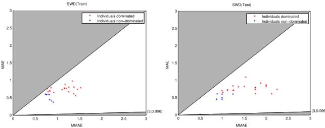
Figure 4 shows the graphical results obtained with
MAE-M MAEpair for the SWD dataset. For theMAE
-M -MAE space, the Pareto front for one specific run of
the 30 ones performed for each dataset is selected, con-cretely the execution that presents the best individual on MAE for training data. The test graphic shows
the M MAE and MAE values over the generalization
set for the individuals who are reflected in the training graphic. Observe that the MAE-M MAEvalues do not form Pareto fronts in generalization, and the individuals
(3,0.096) MMAE MAE SWD(Train) 0 0.5 1 1.5 2 2.5 3 0 0.5 1 1.5 2 2.5 3 Individuals dominated Individuals non−dominated 0 0.5 1 1.5 2 2.5 3 0 0.5 1 1.5 2 2.5 3 Individuals dominated Individuals non−dominated (3,0.096) MMAE MAE SWD(Test)
Figure 4: Pareto front in training and associated values in generalization.
that in the training graphic were in the first Pareto front, now can be located within a worst region. In general, the structure of a Pareto front in training has not to be maintained in generalization.
6. Conclusion
This paper contributes an analysis of different state-of-the-art performance measures to evaluate an ordi-nal classifier. The aim of this aordi-nalysis is selecting the best pair of metrics to guide a multi-objective evolution-ary algorithm. In this analysis, the new M MAE met-ric is included. This metmet-ric is the highest MAE value from MAEs measured independently for each class, i.e. it evaluates the performance of the worst classi-fied class. The analysis studies the correlations between the different metrics for 10 ordinal regression datasets and 4 state-of-the-art methods. Three different pairs of metrics seem to be non-cooperative and, therefore, the most interesting (CCR-M MAE, MAE-M MAEandτb
-M -MAE). In addition, these measures are studied over a
set of synthetic confusion matrices.
To assess these non-cooperative metrics pairs in 10 ordinal datasets, a multi-objective evolutionary algo-rithm called MPDENN is guided by each of these three combinations. The MPDENN is used to optimize a neu-ral network based on the proportional odds model and the results obtained by the extremes of the Pareto fronts when considering each proposal are reported. These re-sults are compared with those obtained for two refer-ence ordinal methods. This comparison establishes the second proposal (MAE-M MAEpair) as a very compet-itive one, obtaining suitable classifiers to optimize all theCCR,MAEandτbmetrics when selecting theMAE
extreme of the Pareto front, and acceptable values of
M MAEwhen selecting the M MAEextreme. The
rea-son of this good performance can be found in the fact that a good ordinal classifier must not only classify well the majority classes but also the other classes, including the smallest ones. Finally, the paper analyses the rela-tionship betweenMAEandM MAEto better understand the 2-dimensional space where the search of the evolu-tionary algorithm takes place. An inequality is derived, which limits the search space, and some of the Pareto fronts are represented both for training and generaliza-tion sets.
Acknowledgment
This work was supported in part by the TIN2011-22794 project of the Spanish Ministerial Commision of Science and Technology (MICYT), FEDER funds and the P08-TIC-3745 project of the “Junta de Andaluc´ıa” (Spain). Manuel Cruz-Ram´ırez’s research has been subsidized by the FPU Predoctoral Program (Spanish Ministry of Education and Science), grant reference AP2009-0487. Javier S´anchez-Monedero’s research has been funded by the “Junta de Andaluc´ıa” Ph. D. Student Program.
References
[1] R. W. Hodge, J. T. Donald, Class identification in the united states, American Journal of Sociology 73 (1968) 535–547. [2] W. Chu, S. S. Keerthi, New approaches to support vector ordinal
regression, in: Proceedings of the 22nd international conference on Machine Learning, 2005, pp. 145–152.
[3] C. Spearman, The proof and measurement of association be-tween two things, American Journal of Psychology 15 (1904) 72–101.
[4] M. G. Kendall, Rank Correlation Methods, New York: Hafner Press, 1962.
[5] L. Goodman, W. Kruskal, Measures of association for cross classifications, Journal of the American Statistical Association 49 (1954) 732–764.
[6] R. H. Somers, The rank analogue of product-moment partial correlation and regression with application to manifold, ordered contingency tables, Biometrika 46 (1955) 241–246.
[7] S. Baccianella, A. Esuli, F. Sebastiani, Evaluation measures for ordinal regression, in: Proccedings of the Ninth International Conference on Intelligent Systems Design and Applications, ISDA’09, 2009, pp. 283–287.
[8] K. Dembczy´nski, W. Kotlowski, R. Slowi´nski, Ordinal
classification with decision rules, in: Proceedings of the
ECML/PKDD’07 workshop on Mining Complex Data, Warsaw,
PL, 2007, pp. 169–181.
[9] J. Weston, S. Bengio, N. Usunier, Large scale image annota-tion: learning to rank with joint word-image embeddings, Mach.
Learn. 81 (1) (2010) 21–35. doi:10.1007/s10994-010-5198-3.
[10] J. Weston, S. Bengio, P. Hamel, Multi-tasking with joint seman-tic spaces for large-scale music annotation and retrieval, Journal of New Music Research 40 (4) (2011) 337–348.
[11] H. Abbass, An evolutionary artificial neural networks approach for breast cancer diagnosis, Artificial Intelligence in Medicine 25 (3) (2002) 265–281.
[12] J. C. Fern´andez, F. Mart´ınez, C. Herv´as, P. A. Guti´errez, Sen-sitivity versus accuracy in multi-class problems using memetic Pareto evolutionary neural networks, IEEE Transactions on Neural Networks 21 (5) (2010) 750–770.
[13] J. S´anchez-Monedero, P. A. Guti´errez, F. Fernandez-Navarro,
C. Herv´as-Mart´ınez, Weighting efficient Accuracy and
Mini-mum Sensitivity for evolving multi-class classifiers, Neural Pro-cessing Letters 34 (2) (2011) 1370–4621.
[14] M. Cruz-Ram´ırez, C. Herv´as-Mart´ınez, J. Fernandez-Caballero, J. Brice˜no, M. de la Mata, Multi-Objective Evolutionary Al-gorithm for Donor-Recipient Decision System in Liver Trans-plants, European Journal of Operational Research 222 (2) (2012) 317–327.
[15] W. Waegeman, B. D. Baets, L. Boullart, ROC analysis in ordinal regression learning, Pattern Recognition Letters 29 (1) (2008) 1–9.
[16] P. McCullagh, Regression models for ordinal data, Journal of the Royal Statistical Society, Series B (Methodological) 42 (2) (1980) 109–142.
[17] R. Storn, K. Price, Differential Evolution. A fast and efficient
heuristic for global optimization over continuous spaces, Journal of Global Optimization 11 (1997) 341–359.
[18] H. A. Abbass, R. Sarker, C. Newton, PDE: a Pareto-frontier
differential evolution approach for multi-objective optimization
problems, in: Proceedings of the 2001 Congress on Evolution-ary Computation, Vol. 2, Seoul, South Korea, 2001, pp. 971– 978.
[19] M. Cruz-Ram´ırez, C. Herv´as-Mart´ınez, J. S´anchez-Monedero, P. A. Gutierrez, A preliminary study of ordinal metrics to guide a multi-objective evolutionary algorithm, in: 11th International Conference on Intelligent Systems Design and Applications, ISDA 2011, C´ordoba, Spain, 2011, pp. 1176–1181.
[20] C. Igel, M. H¨usken, Empirical evaluation of the improved rprop learning algorithms, Neurocomputing 50 (6) (2003) 105–123. [21] J. L. Fleiss, J. Cohen, B. S. Everitt, Large sample standard
er-rors of kappa and weighted kappa, Psychological Bulletin 72 (5) (1969) 323–327.
[22] C.-C. Chang, C.-J. Lin, LibSVM: A library for support vector machines, ACM Trans. Intell. Syst. Technol. 2 (3) (2011) 1–27. [23] L. Li, H. T. Lin, Ordinal regression by extended binary
classifi-cation, Advances in Neural Information Processing Systems 19 (2007) 865–872.
[24] W. Chu, S. S. Keerthi, Support Vector Ordinal Regression, Neu-ral Computation 19 (3) (2007) 792–815.
[25] J. S. Cardoso, R. Sousa, Measuring the performance of ordinal classification, International Journal of Pattern Recognition and Artificial Intelligence 25 (8) (2011) 1173–1195.
[26] M. Dorado-Moreno, P. A. Guti´errez, C. Herv´as-Mart´ınez, Or-dinal Classification Using Hybrid Artificial Neural Networks with Projection and Kernel Basis Functions, in: 7th Interna-tional Conference on Hybrid Artificial Intelligence Systems (HAIS2012), 2012, pp. 319–330.
[27] J. Verwaeren, W. Waegeman, B. De Baets, Learning partial or-dinal class memberships with kernel-based proportional odds models, Computational Statistics & Data Analysis 56 (4) (2012) 928–942.
[28] M. Cruz-Ram´ırez, C. Herv´as-Mart´ınez, P. A. Guti´errez, M. P´erez-Ortiz, J. Brice˜no, M. de la Mata, Memetic Pareto dif-ferential evolutionary neural network used to solve an unbal-anced liver transplantation problem, Soft Computing 17 (2012) 275–284.
[29] J. C. Fern´andez, C. Herv´as, F. J. Mart´ınez, P. A. Guti´errez,
M. Cruz, Memetic Pareto differential evolution for designing
artificial neural networks in multiclassification problems using cross-entropy versus sensitivity, in: Proceedings of the 4th In-ternational Conference, HAIS 2009, Vol. 5572, Springer-Verlag Berlin, Heidelberg, 2009, pp. 433–441.
[30] J.-X. Du, D.-S. Huang, X.-F. Wang, X. Gu, Shape recognition
based on neural networks trained by differential evolution
algo-rithm, Neurocomputing 70 (4-6) (2007) 896–903.
[31] B. Subudhi, D. Jena, Nonlinear system identification using
memetic differential evolution trained neural networks,
Neuro-computing 74 (10) (2011) 1696–1709.
[32] M. Cruz-Ram´ırez, C. Herv´as-Mart´ınez, M. Jurado-Exp´osito, F. L´opez-Granados, A multi-objective neural network based method for cover crop identification from remote sensed data, Expert Systems with Applications 39 (11) (2012) 10038 – 10048.
[33] C. Bishop, Pattern Recognition and Machine Learning,
Springer, 2006.
[34] J. Pinto da Costa, J. Cardoso, Classification of ordinal data using neural networks, in: Proceedings of the 16th European confer-ence on Machine Learning, ECML’05, Springer-Verlag, 2005, pp. 690–697.
[35] M. Mathieson, Ordinal models for neural networks, in: Neural networks in financial engineering. Proceedings of the 3rd inter-national conference on Neural networks in the capital markets, London, GB, October, 1995, Singapore: World Scientific, 1996, pp. 523–536.
[36] J. Demsar, Statistical comparisons of clasiffiers over multiple
data sets, Journal of Machine Learning Research 7 (2006) 1–30. [37] M. Friedman, A comparison of alternative tests of significance for the problem of m rankings, Annals of Mathematical Statis-tics 11 (1) (1940) 86–92.
[38] Y. Hochberg, A. Tamhane, Multiple Comparison Procedures, John Wiley & Sons, Inc. New York, NY, USA, 1987.