Improvements in ranked set sampling

(1)

IMPROVEMENTS IN RANKED SET SAMPLING

A thesis submitted in partial fulfilment of the requirements for the degree of Doctor of Philosophy in Statistics

at the University of Canterbury by ABDUL HAQ

School of Mathematics and Statistics University of Canterbury, Christchurch

(2)

(3)

Abstract

The main focus of many agricultural, ecological and environmental studies is to develop well designed, cost-effective and efficient sampling designs. Ranked set sampling (RSS) is one of those sampling methods that can help accomplish such objectives by incorporating prior information and expert knowledge to the design. In this thesis, new RSS schemes are suggested for efficiently estimating the population mean. These sampling schemes can be used as cost-effective alternatives to the traditional simple random sampling (SRS) and RSS schemes. It is shown that the mean estimators under the proposed sampling schemes are at least as efficient as the mean estimator with SRS. We consider the best linear unbiased estimators (BLUEs) and the best linear invariant estimators (BLIEs) for the unknown parameters (location and scale) of a location-scale family of distributions under double RSS (DRSS) scheme. The BLUEs and BLIEs with DRSS are more precise than their counterparts based on SRS and RSS schemes. We also consider the BLUEs based on DRSS and ordered DRSS (ODRSS) schemes for the unknown parameters of a simple linear regression model using replicated observations. It turns out that, in terms of relative efficiencies, the BLUEs under ODRSS are better than the BLUEs with SRS, RSS, ordered RSS (ORSS) and DRSS schemes.

Quality control charts are widely recognized for their potential to be a powerful process monitoring tool of the statistical process control. These control charts are frequently used in many industrial and service organizations to monitor in-control and out-of-control performances of a production or manufacturing process. The RSS schemes have had considerable attention in the construction of quality control charts. We propose new exponentially weighted moving average (EWMA) control charts for monitoring the process mean and the process dispersion based on the BLUEs obtained under ORSS and ODRSS schemes. We also suggest an improved maximum EWMA control chart for simultaneously monitoring the process mean and dispersion based on the BLUEs with ORSS scheme. The proposed EWMA control charts perform substantially better than their counterparts based on SRS and RSS schemes. Finally, some new EWMA charts are also suggested for monitoring the process dispersion using the best linear unbiased absolute estimators of the scale parameter under SRS and RSS schemes.

(4)

(5)

Dedication

To the memory of

‘Al-Sayed Muhiyuddin Abu Muhammad Abdul Qadir Al-Gilani Al-Hasani Wal-Hussaini’ (RA), Ghaus-e-Aazam, Baghdad, Iraq.

(6)

(7)

Acknowledgments

In The Name of Allah, The Most Gracious, The Most Merciful.

“He is Allah, other than whom there is no deity, Knower of the unseen and the witnessed. He is the Entirely Merciful, the Especially Merciful.” — Holy Quran 59:21.

First and foremost, I’m extremely thankful to The Almighty Allah for blessing, protecting and guiding me throughout this period to complete this task. All my respect and love go to The Prophet Muhammad (peace be upon him), who once said

“Learning is from cradle to grave—seek knowledge even if it is in China.”

I express my profound sense of reverence to my supervisors, Prof. Jennifer Brown and Dr. Elena Moltchanova, for their constant guidance, support, time, motivation and help during the course of my PhD. I’m very thankful to Prof. Jennifer Brown for giving me freedom during my research, having trust in my abilities, and she’s always been very kind and nice to me.

I’m also thankful to the University of Canterbury (UoC) for financially supporting my PhD research through “University of Canterbury International Doctoral Scholarship”. Without this support, it’d have been very difficult for me to get the PhD from UoC, Christchurch, New Zealand. Thanks are also extended to all the administration staff at the School of Mathematics and Statistics, UoC.

Last but not the least, I cheerfully express my profound thanks to my parents, grand parents, my brother and sisters, teachers and friends for their support, help and cooperation during my work.

(8)

(9)

List of Figures

1.1 REs of PRSS with respect to SRS for estimating population mean under perfect and imperfect rankings . . . 5 1.2 REs of PRSS with respect to SRS for estimating population median under perfect and imperfect

rankings . . . 7 1.3 REs of PRSS with respect to SRS for estimating population variance under perfect and

imperfect rankings . . . 8 2.1 REs of mean estimators based on PRSS and MxRSS versus SRS for symmetric distributions . 18 2.2 REs of mean estimators based on PRSS and MxRSS versus SRS for asymmetric distributions 19 2.3 REs of mean estimators based on IPRSS and IMxRSS versus SRS for standard bivariate

normal distribution . . . 20 2.4 EREs of median estimators based on PRSS and MxRSS versus SRS for symmetric distributions 21 2.5 EREs of median estimators based on PRSS and MxRSS versus SRS for asymmetric distributions 22 4.1 Comparison of EMSEs of BLUEs and BLIEs based on IRSS versus IDRSS when m= 5 . . . 66 6.1 Comparison of the EWMA-ORSS location control chart with some classical EWMA charts

based on SRS . . . 113 6.2 Comparison of EWMA-OIRSS location chart with some classical EWMA charts based on SRS 113 6.3 Comparison of EWMA-ORSS location control charts versus Shewhart-CUSUM-RSS and

Shewhart-EWMA-RSS control charts . . . 114 6.4 Comparison of the proposed EWMA-ORSS chart versus CS-EWMA-SRS chart for monitoring

process dispersion . . . 115 6.5 Comparison of EWMA-ORSS scale control chart versus EWMA control charts for monitoring

process dispersion . . . 116 6.6 Comparison of one-sided EWMA-ORSS and EWMA-OIRSS charts versus one-sided EWMA

dispersion control charts . . . 117 6.7 Comparison of the Shewhart-EWMA-RSS and EWMA-ORSS location control charts for real

data . . . 118 6.8 Comparison of the CS-EWMA-SRS and EWMA-ORSS dispersion control charts for real data 119 7.1 Comparison of the MaxEWMA-SRS, MaxGWMA-SRS and MaxEWMA-ORSS control charts

for piston rings data . . . 146 8.1 Comparison of the EWMA-ODRSS mean chart with some classical and recent EWMA mean

charts . . . 169 8.2 Comparison of the EWMA-OIDRSS mean chart with some classical and recent EWMA mean

(14)

8.3 Comparison of the EWMA-OIDRSS mean chart versus combined Shewhart-EWMA-RSS, combined Shewhart-EWMA-MRSS and EWMA-ORSS mean charts . . . 171 8.4 Comparison of the two-sided EWMA-ODRSS dispersion chart versus two-sided EWMA

dispersion charts . . . 172 8.5 Comparison of the one-sided EWMA-ODRSS dispersion chart versus one-sided EWMA

dispersion charts . . . 173 8.6 Comparison of the one-sided EWMA-OIDRSS dispersion chart versus one-sided EWMA

dispersion charts . . . 173 8.7 EWMA-ODRSS and EWMA-ORSS mean charts for simulated data . . . 174 8.8 EWMA-ODRSS and EWMA-ORSS dispersion charts for simulated data . . . 175 9.1 Comparison of the two-sided EWMA control charts when EWMA-SRS and EWMA-RSS charts

are based on the symmetric control limits . . . 198 9.2 Comparison of the two-sided EWMA control charts when EWMA-SRS and EWMA-RSS charts

are based on the asymmetric control limits . . . 198 9.3 Comparisons of the one-sided EWMA control charts for monitoring increases in the process

dispersion . . . 199 9.4 Comparisons of the one-sided EWMA control charts for monitoring decreases in the process

dispersion . . . 200 9.5 Comparisons of the two-sided EWMA control charts when EWMA-IRSS chart is based on

asymmetric control limits . . . 200 9.6 Comparisons of the one-sided EWMA control charts with EWMA-IRSS control chart for

monitoring increases in the process dispersion . . . 201 9.7 Comparisons of the one-sided EWMA control charts with EWMA-IRSS control chart for

monitoring decreases in the process dispersion . . . 201 9.8 Comparison of the HHW1-EWMA and HHW2-EWMA control charts for real data . . . 202 9.9 Comparison of the EWMA-SRS and EWMA-RSS control charts for real data . . . 203

(15)

List of Tables

1.1 Summary statistics of 399 trees data . . . 9

1.2 Estimation of the population mean, median and variance of the study variableX under perfect and imperfect rankings . . . 10

2.1 Summary statistics of 399 trees data . . . 23

2.2 Comparison of EBs and EREs of the mean and median estimators based on perfect and imperfect PRSS schemes with respect to their counterparts based on SRS for trees data . . . 23

2.3 Comparison of EBs and EREs of the mean and median estimators based on perfect and imperfect MxRSS schemes with respect to their counterparts based on SRS for trees data . . 24

3.1 Exact RPs relative to SRS under symmetric and asymmetric distributions . . . 41

3.2 Exact RPs relative to SRS under imperfect ranking . . . 41

3.3 Exact RPs of estimators under perfect ranking relative to SRS-based regression estimator . . 42

3.4 Exact RPs of estimators under imperfect ranking relative to SRS-based regression estimator . 43 3.5 Summary statistics of 399 trees data . . . 44

3.6 ERPs relative to SRS for trees data . . . 44

4.1 Means of the order statistics from different sample sizes under RSS and DRSS . . . 61

4.2 Variances of the order statistics from different sample sizes under RSS and DRSS . . . 62

4.3 The values of coefficients needed for computing the BLUEs ofµandσunder DRSS . . . 63

4.4 REs of BLUEs and BLIEs under RSS and DRSS . . . 64

4.5 REs of BLUEs and BLIEs under IRSS versus IDRSS . . . 65

4.6 EREs of BLUEs and BLIEs under IRSS and IDRSS . . . 67

4.7 REs of quantile estimators based on BLUE and BLIE under perfect and imperfect rankings . 73 4.8 REs of quantile estimators based on BLUE and BLIE of RSS versus DRSS under perfect and imperfect rankings . . . 74

5.1 Means of order statistics from symmetric distributions under different sampling schemes . . . 84

5.2 Variances and Covariances of order statistics from symmetric distributions under OSRS . . . 85

5.3 Variance and Covariance of order statistics from symmetric distributions under ORSS . . . . 86

5.4 Variances and Covariances of order statistics from symmetric distributions under ODRSS . . 87

5.5 REs of BLUEs based on OSRS, RSS, ORSS, DRSS and ODRSS schemes . . . 87

5.6 REs of BLUEs based on OSRS, RSS, ORSS, DRSS, ODRSS for scale contaminated normal distributions . . . 88

5.7 Trace REs of BLUEs based on RSS, ORSS, DRSS, ODRSS relative to OSRS for normal distribution . . . 88

5.8 Trace REs of BLUEs based on RSS, ORSS, DRSS, ODRSS relative to OSRS for Laplace distribution . . . 89

(16)

5.9 Trace REs of BLUEs based on RSS, ORSS, DRSS, ODRSS relative to OSRS for scale

contaminated normal distribution with= 0.01 . . . 89

5.10 Trace REs of BLUEs based on RSS, ORSS, DRSS, ODRSS relative to OSRS for scale contaminated normal distribution with= 0.05 . . . 90

5.11 Trace REs of BLUEs based on RSS, ORSS, DRSS, ODRSS relative to OSRS for scale contaminated normal distribution with= 0.10 . . . 90

5.12 EMSEs of unknown parameters of SLRM under RSS schemes for normal distribution . . . 91

5.13 EMSEs of unknown parameters of SLRM under RSS schemes for Laplace distribution . . . . 91

5.14 EMSEs of unknown parameters of SLRM under RSS schemes for scale contaminated normal distribution with= 0.05 . . . 92

5.15 REs of the BLUEs under different RSS schemes when normality assumptions do not hold . . 96

6.1 Run length properties of EWMA-ORSS (two-sided) process mean control chart . . . 104

6.2 Run length properties of EWMA-OIRSS (two-sided) process mean control chart . . . 105

6.3 Run length properties of the EWMA-ORSS (two-sided) dispersion control chart . . . 107

6.4 Run length properties of EWMA-ORSS (one-sided) dispersion control chart . . . 108

6.5 Run length properties of EWMA-OIRSS (two-sided) dispersion chart . . . 110

6.6 Run length properties of EWMA-OIRSS (one-sided) dispersion control chart . . . 112

7.1 ARLs and SDRLs of the MaxEWMA-ORSS control chart when in-control ARL is fixed to 185 134 7.2 ARLs and SDRLs of the MaxEWMA-ORSS control chart when in-control ARL is fixed to 250 135 7.3 ARLs and SDRLs of the MaxEWMA-ORSS control chart when in-control ARL is fixed to 370 136 7.4 ARLs and SDRLs of the OIRSS control chart when in-control ARL of MaxEWMA-ORSS chart is fixed to 185 . . . 137

7.5 ARLs and SDRLs of the OIRSS control chart when in-control ARL of MaxEWMA-ORSS chart is fixed to 250 . . . 138

7.6 ARLs and SDRLs of the OIRSS control chart when in-control ARL of MaxEWMA-ORSS chart is fixed to 370 . . . 139

7.7 A comparison of ARLs and SDRLs of the MaxEWMA-ORSS (ξ = 0.05) with optimal MaxEWMA-SRS and optimal MaxGWMA-SRS charts when in-control ARL is fixed to 185 . 140 7.8 A comparison of ARLs and SDRLs of the MaxEWMA-ORSS (ξ = 0.05) with optimal MaxEWMA-SRS and optimal MaxGWMA-SRS charts when in-control ARL is fixed to 250 . 141 7.9 A comparison of ARLs and SDRLs of the MaxEWMA-ORSS (ξ = 0.05) with optimal MaxEWMA-SRS and optimal MaxGWMA-SRS charts when in-control ARL is fixed to 370 . 142 7.10 ARLs and SDRLs of the MaxEWMA-OIRSS chart versus optimal MaxEWMA-SRS and optimal MaxEWMA-GWMA-SRS control charts when in-control ARL is fixed to 370 . . . 143

7.11 A comparison of diagnostic abilities of the MaxGWMA-SRS and MaxEWMA-ORSS control charts when in-control ARL is fixed to 370 . . . 144

8.1 Run length properties of the EWMA-ODRSS process mean control chart . . . 158

8.2 Run length properties of the EWMA-OIDRSS process mean control chart . . . 159

8.3 Run length properties of the EWMA-ODRSS dispersion chart . . . 160

8.4 Run length properties of the EWMA-ODRSS (one-sided) dispersion charts . . . 163

8.5 Run length properties of the EWMA-OIDRSS (two-sided) dispersion charts . . . 165

8.6 Run length properties of the EWMA-OIDRSS (one-sided) dispersion chart for monitoring increases in the process dispersion . . . 167

8.7 Run length properties of the EWMA-OIDRSS (one-sided) dispersion chart for monitoring decreases in the process dispersion . . . 168

(17)

LIST OF TABLES xvii

9.1 Run length characteristics of the two-sided EWMA-SRS control chart . . . 185

9.2 Run length characteristics of the one-sided EWMA-SRS control charts . . . 186

9.3 Run length characteristics of the two-sided EWMA-RSS control chart . . . 190

9.4 Run length characteristics of the one-sided EWMA-RSS control charts . . . 191

9.5 Run length characteristics of the two-sided EWMA-IRSS control chart . . . 193

9.6 Run length characteristics of the one-sided EWMA-IRSS chart when detecting increases in the process dispersion . . . 195

9.7 Run length characteristics of the one-sided EWMA-IRSS chart when detecting decreases in the process dispersion . . . 196

(18)

(19)

Preface

This thesis is a collection of research articles on improvements in ranked set sampling (RSS). All of the chapters have been either published or accepted for publication in different international journals, including Environmetrics, Journal of Applied Statistics, Communications in Statistics-Theory and Methods, and Quality and Reliability Engineering International. Since each chapter is an independent research article focusing on RSS, there are some repetitions in the form of RSS methods, literature review and notations.

The outline of the thesis is as follows: In Chapter 1, we propose a cost-effective sampling scheme, named partial RSS (PRSS), for estimating the population mean, median and variance. The PRSS scheme selects samples using both simple random sampling (SRS) and RSS schemes, and thus reduces the cost of ranking. In Chapter 2, we extend the work on PRSS, and propose a mixed RSS (MxRSS) scheme, as a cost-effective alternative to the RSS scheme, for estimating the population mean and median. The MxRSS scheme encompasses both SRS and RSS schemes, and it helps in selecting more representative samples from the parent population. Under MxRSS scheme, there are more possibilities to select a sample than those with the PRSS scheme. It is shown that the MxRSS scheme, generally, provides more efficient mean and median estimators than those with SRS and PRSS schemes. Chapter 3 further extends this work, and suggests a new paired double RSS (PDRSS) scheme, as a cost-effective alternative to the double RSS (DRSS) scheme, for estimating the population mean. The mean estimator under PDRSS scheme is at least as efficient as the mean estimator based on RSS. Note that in Chapter 3 we use the notation “PRSS” for paired RSS scheme, and it should not be confused with the notation of the partial RSS (PRSS) scheme used in Chapters 1 and 2. In Chapter 4, we derive the best linear unbiased and invariant estimators for the unknown parameters (location and scale) of a location-scale family of distributions under DRSS scheme. Chapter 5 proposes the best linear unbiased estimators (BLUEs) for the unknown parameters of a simple linear regression model with replicated observations using DRSS and ordered DRSS (ODRSS) schemes.

In Chapter 6, we suggest new exponentially weighted moving average (EWMA) control charts for monitoring the process mean and the process dispersion using the BLUEs (location and scale) obtained under ordered RSS (ORSS). In Chapter 7, we extend the work on ORSS scheme, and suggest an improved maximum EWMA control chart for simultaneously monitoring the process mean and dispersion. Chapter 8 extends the work on ODRSS scheme, and proposes new EWMA control charts based on the BLUEs (location and scale) using ODRSS for monitoring the process mean and the process dispersion. In Chapter 9, we suggest new

(20)

EWMA control charts based on the best linear unbiased absolute estimators of the scale parameter under SRS and RSS schemes for monitoring the process dispersion.

(21)

Chapter 1

Partial Ranked Set Sampling Design

This chapter appeared in:

Haq, A., Brown, J., Moltchanova, E., Al-Omari, A.I., 2013, Partial ranked set sampling design, Environmetrics, 24(3), 201–207.

In many environmental studies, the main focus is on observational economy, that is, to obtain data on the basis of cost-effective and efficient sampling methods. In this chapter, we propose a partial ranked set sampling (PRSS) method for estimation of population mean, median and variance. On the basis of perfect and imperfect rankings, Monte Carlo simulations from symmetric and asymmetric distributions are used to evaluate the effectiveness of the proposed estimators. It is found that the estimators under PRSS are more efficient than the estimators based on simple random sampling. The procedure is illustrated with a case study using a real data set

1.1

Introduction

In many studies where sampling is used, such as environmental management, ecology, sociology and agriculture, exact measurement of a selected unit is either difficult or costly and time-consuming. However, the ranking of a small set of selected units can be carried out easily either by visual inspection with respect to the study variable or on the basis of auxiliary variable. For example, hazardous waste sites with different levels of contamination can be ranked by a visual inspection of soil discoloration, whereas the actual measurements of toxic chemicals and quantifying their environmental impact is very costly. McIntyre (1952) proposed a method, later called ranked set sampling (RSS), for estimating mean pasture and forage yields when measurement is costly. Takahasi and Wakimoto (1968) derived the statistical theory of the RSS procedure. Dell and Clutter (1972) showed that under imperfect ranking, the sample mean remains an unbiased estimator of the population mean, but ranking should be better than at least a random ordering. As mentioned by

(22)

Stokes (1977), the concomitant variables can be used to judge the ranks of the study variable. For a detailed review and bibliography on RSS, see Patil (1995) and Kaur et al. (1995). For some real applications of RSS, see Yu and Lam (1997), Al-Saleh and Al-Shrafat (2001), Al-Saleh and Al-Hadrami (2003), Al-Saleh and Al-Omari (2002), Husby et al. (2005), Chen (2007), Wang et al. (2009), Ozturk (2011), Samawi (2011) and references therein.

Under the RSS scheme, the experimenter selects m random samples, each of size m, from the target population. The units within each sample are ranked visually without actual measurements. This may be difficult when the data arrive in batches of varying sizes or when the ranking is difficult and results in large inaccuracies or is time-consuming. An initial sample of m2 experimental units under RSS produces the final sample ofm units.

In this chapter, we propose a cost-effective sampling method, namely partial ranked set sampling (PRSS) design. This design provides flexibility to the experimenter in selecting the sample when it is either difficult to rank the units within each set with full confidence or due to non-availability of experimental units. Under the PRSS scheme, the experimenter selectsAunits using simple random sampling (SRS) andB units using the RSS, producing the final sample of sizem=A+B units. It thus requires less sampling units and less ranking than the RSS and proves to be more efficient than SRS.

The rest of the chapter is organized as follows: In Section 1.2, the RSS and PRSS methods are described. Estimation of the population mean is considered in Section 1.3. In Section 1.4, the PRSS is considered for median and variance estimation. An application to real data set is given in Section 1.5. Finally, we summarize our results in Section 1.6.

1.2

Sampling methods

In this section, we explain the RSS and PRSS procedures.

1.2.1

Ranked set sampling

The RSS can be described as follows: identifym2 units from the target population. Randomly allocate these units intomsets, each of sizem. The units within each set are ranked visually or by any inexpensive method with respect to the variable of interest. From the first set ofmunits, the smallest ranked unit is measured; the second smallest ranked unit is measured from the second set of munits. The process continues until the mth smallest ranked unit is measured from the last set. The process can be repeatedrnumber of times to obtain a large sample of sizemr.

Let the study variableX has a probability density function (PDF) f(x) and cumulative distribution function F(x), with mean µ and variance σ2. Let X₁, X₂, ..., Xm be a simple random sample of size m drawn fromf(x). The SRS estimator of µis ¯X_SRS= _m1 Pm

i=1Xi with variance Var( ¯XSRS) = σ2

m. Consider X₁₁, X₁₂, ..., X₁m, X₂₁, X₂₂, ..., X₂m, ..., Xm₁, Xm₂, ..., Xmm bemindependent simple random samples each of sizem. LetXi(1:m), Xi(2:m), ..., Xi(m:m)represent the order statistics of theith sample. Using RSS scheme,

(23)

1.2 Sampling methods 3

the measured RSS units are denoted byX_1(1:m), X2(2:m), ..., Xm(m:m). Letg(i:m)(x) be the PDF of theith order statistic, i.e.,X₍i_:m₎,i= 1,2, ..., m, from a random sample of sizem. It can be shown that

g₍i_:m₎(x) =m

_m₋1

i−1

{F(x)}i−1{1−F(x)}m−if(x), −∞< x <+∞,

see David and Nagaraja (2003).

The mean and variance of X₍i:m), respectively, are

µ₍i:m)= ∞ Z −∞ xg₍i:m)(x)dx and σ2₍i:m)= ∞ Z −∞ (x−µ₍i:m))2g(i:m)(x)dx.

The RSS estimator of the population mean is ¯ X_RSS= 1 m m X i=1 Xi(i:m), with variance Var( ¯X_RSS) = 1 m2 m X i₌₁ σ2₍_i_:_m₎= σ 2 m − 1 m2 m X i₌₁ (µ₍i:m)−µ)2.

1.2.2

Partial ranked set sampling

The PRSS scheme is a mixture of both SRS and RSS designs. We propose this design for use when the experimenter is unable to inspect the number of units that are required for a balanced ranked set sample or when inspection cost per unit is high. The PRSS scheme requires fewer identified units as compared with a ranked set sample, and at the same time, it provides more precise estimates than the commonly used SRS scheme. Thus, PRSS scheme helps in reducing the total cost and expenditure that is involved in sampling.

In order to select a partial ranked set sample of sizem, the following steps are carried out:

Step 1: Define a coefficientk such thatk= [αm], where 0≤α <0.5. Here, [t] represents the largest integer value less than or equal tot.

Step 2: Select 2k simple random samples each of size one from the parent population. In order to select the remaining m−2k units, selectm−2ksets each of size mfrom the parent population. Rank the units within each set and select theith ranked unit of theith sample, fori=k+ 1, ..., m−k. This completes one cycle of a partial ranked set sample of sizem.

Step 3: The above Steps 1 and 2 can be repeatedrtimes in order to select a partial ranked set sample of sizen=mr.

The total number of units that were involved in selecting a partial ranked set sample of sizemarem2−2k(m−1).

(24)

1.3

Estimation of population mean

Let X₁₁, X₁₂, ..., X₁m, X21, X22, ..., X2m, ..., Xm1, Xm2, ..., Xmm be m independent simple random samples each of size m. Apply the PRSS procedure on thesemsamples, as explained in Section 1.2.2. The PRSS estimator of population mean is defined as

¯ X_PRSS= 1 m k X i=1 Xi+ m−k X i=k+1 Xi(i:m)+ m X i=m−k+1 Xi ! , with variance Var( ¯X_PRSS) =2kσ 2 m2 + 1 m2 m−k X i=k+1 σ2₍_i_:_m₎.

For a symmetric distribution, we haveµ₍i:m)+µ(m−i+1:m)= 2µandσ₍2i:m)=σ(2m−i+1:m), fori= 1,2, ..., m, see David and Nagaraja (2003). Then, it is easy to show E( ¯X_PRSS) = µ, Var( ¯X_PRSS) = Var( ¯X_RSS) +

2

m2

Pk

i=1(σ2−σ₍2i_:m₎). Also, Var( ¯XPRSS)≤Var( ¯XSRS) if and only ifσ2≥ m−12k

Pm−k

i=k+1σ₍2i_:m₎. For a symmetric population, the relative efficiency (RE) of ¯X_PRSS with respect to ¯X_SRSis

RE( ¯X_PRSS,X¯_SRS) = Var( ¯XSRS) Var( ¯X_PRSS) = mσ2 2kσ2+Pm−k i=k+1σ2₍i:m) .

Similarly, for an asymmetric population, the RE will be RE( ¯X_PRSS,X¯_SRS) = Var( ¯XSRS) MSE( ¯X_PRSS)= mσ2 2kσ2+Pm−k i₌k₊₁σ₍2i:m)+m2{E( ¯XPRSS−µ)}2 ,

where MSE is the mean squared error.

1.3.1

Simulation study for mean estimation

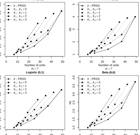
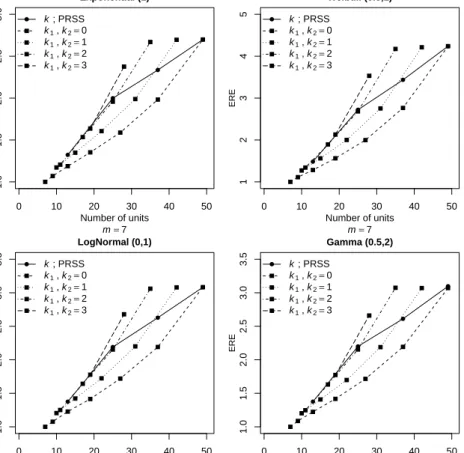
In this section, a simulation study is conducted to investigate the efficiency of PRSS for estimating the population mean with m = 4,5,6,7. The RE is used as a performance criterion for estimators. We consider symmetric distributions: Normal (0,1), Uniform (0,1), Logistic (0,1) and Beta (6,6) and asymmetric distributions: Exponential (1), Weibull (0.5,1), Lognormal (0,1) and Gamma (0.5,1). The sampling schemes (SRS and PRSS) are based on the same sample size. Under each sampling scheme, for given values ofmand k, from each distribution, one million estimates ofµand their MSEs are estimated. The estimated REs are calculated and displayed in Figure 1.1.

(a) Univariate case

For all the distributions considered in this study, the mean estimators based on PRSS are more efficient than the estimators from SRS (RE>1). It is observed that as the value ofm increases, the RE of mean estimator based on PRSS also increases and vice-versa. For symmetric distributions, with fixed m, the RE decreases as the value of kincreases. In asymmetric distributions, the RE increases asmincreases, but at

(25)

1.3 Estimation of population mean 5 10 20 30 40 50 1 2 3 4 5 RSS k=0 PRSS k=1 PRSS k=2 PRSS k=3 Number of units Relativ e Efficiency Normal(0,1) 10 20 30 40 50 1 2 3 4 5 RSS k=0 PRSS k=1 PRSS k=2 PRSS k=3 Number of units Relativ e Efficiency Uniform(0,1) 10 20 30 40 50 1 2 3 4 5 RSS k=0 PRSS k=1 PRSS k=2 PRSS k=3 Number of units Relativ e Efficiency Logistic(0,1) 10 20 30 40 50 1 2 3 4 5 RSS k=0 PRSS k=1 PRSS k=2 PRSS k=3 Number of units Relativ e Efficiency Beta(6,6) 10 20 30 40 50 1.0 1.5 2.0 2.5 3.0 3.5 4.0 _{RSS k}₌₀ PRSS k=1 PRSS k=2 PRSS k=3 Number of units Relativ e Efficiency Exponential(1) 10 20 30 40 50 1.0 1.5 2.0 2.5 3.0 3.5 4.0 _{RSS k}₌₀ PRSS k=1 PRSS k=2 PRSS k=3 Number of units Relativ e Efficiency Weibull(0.5,1) 10 20 30 40 50 1.0 1.5 2.0 2.5 3.0 3.5 4.0 _{RSS k}₌₀ PRSS k=1 PRSS k=2 PRSS k=3 Number of units Relativ e Efficiency Lognormal(0,1) 10 20 30 40 50 1.0 1.5 2.0 2.5 3.0 3.5 4.0 _{RSS k}₌₀ PRSS k=1 PRSS k=2 PRSS k=3 Number of units Relativ e Efficiency Gamma(0.5,2) 10 20 30 40 50 1 2 3 4 5 RSS k=0 PRSS k=1 PRSS k=2 PRSS k=3 Number of units Relativ e Efficiency ρ =0.99 10 20 30 40 50 1.0 1.5 2.0 2.5 _{RSS k}₌₀ PRSS k=1 PRSS k=2 PRSS k=3 Number of units Relativ e Efficiency ρ =0.80 10 20 30 40 50 1.0 1.1 1.2 1.3 1.4 1.5 _{RSS k}₌₀ PRSS k=1 PRSS k=2 PRSS k=3 Number of units Relativ e Efficiency ρ =0.50 10 20 30 40 50 1.00 1.02 1.04 1.06 1.08 1.10 RSS k=0 PRSS k=1 PRSS k=2 PRSS k=3 Number of units Relativ e Efficiency ρ =0.20

Figure 1.1: REs of PRSS with respect to SRS for estimating population mean under perfect and imperfect rankings

the same time, it also depends on the valuek. The RSS mean estimator is more precise than the PRSS mean estimator because it uses more numbers of units. It is of interest to note that when the underlying distribution is asymmetric like Weibull (0.5,1) or Lognormal (0,1), the RE of PRSS mean estimator is higher as compared with the RSS mean estimator. From Section 1.3, we have

MSE( ¯X_PRSS) = Var( ¯X_RSS) + 1 m2{2σ

2₋₍_σ2

(1:m)+σ2(m:m))}+{Bias( ¯XPRSS)}2, fork= 1.

Note that for some highly skewed distributions, 2σ2<(σ2_(1:_m₎+σ₍2_m_:_m₎), as a result of which MSE( ¯X_PRSS)≤

Var( ¯X_RSS). Moreover, the PRSS scheme uses fewer units to achieve higher efficiency.

(b) Bivariate case

In most of the real life situations, it is difficult to rank the study variable visually or it is too costly. In such environments, it is beneficial to use any auxiliary variable that is highly correlated with the study variable.

(26)

In order to investigate the performances of the estimators under the PRSS design, we assume that both the study and the auxiliary variables follow a standard bivariate normal distribution, having PDF:

fX,Y(x, y) = 1 2πp1−ρ2exp −(x 2₋₂_ρxy₊_y2₎ 2(1−ρ2) , −∞< x, y <+∞.

Different values of the correlation coefficient, ρ = 0.99,0.80,0.50,0.20, were considered. Here, we have assumed that the ranking on the auxiliary variable Y is perfect, whereas there are errors in ranking the study variable X. On the basis of extensive Monte Carlo simulations, the REs are calculated and displayed in Figure 1.1.

We can conclude that even when the ranking of the study variable is imperfect, PRSS is more efficient than SRS in estimating the population mean ofX. Also, the RE increases with an increase in the value ofm, whereas it is a decreasing function ofk. The value of ρplays a key role in the performance of the PRSS mean estimator. As the value of ρincreases, the efficiency of PRSS estimator also increases as compared with the estimator under SRS.

1.4

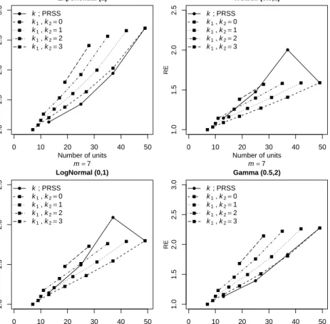
Estimation of population median and variance

The median is often considered as a more suitable measure of location than the mean when the underlying population is highly skewed such as income, expenditure and production. In this section, we compare the estimators of population median and variance on the basis of SRS, RSS and PRSS methods.

We use Monte Carlo simulations from both symmetric and asymmetric distributions to compare the REs of the median and variance estimators. The standard bivariate normal distribution is also used to study the impact of imperfect ranking on the proposed median estimator under PRSS.

The SRS estimator of the population median is defined as ˆ θ_SRS= Median{X₁, X₂, ..., Xm}=      X₍₍m+1)/2:m), ifmis odd, {X₍m/2:m)+X((m+2)/2:m)}/2, ifmis even.

Similarly, the median estimator under PRSS is defined as ˆ

θ_PRSS= Median{X₁, ..., Xk, Xk+1(k+1:m), ..., Xm−k(m−k:m), Xm−k+1, ..., Xm}.

The RE of ˆθ_PRSSwith respect to ˆθ_SRSis RE(ˆθ_PRSS,θˆ_SRS) = MSE(ˆθSRS)

MSE(ˆθPRSS). The estimated MSE of any estimator, say ˆθJ, is MSE(ˆθJ) = _N1 P

N

i₌₁(ˆθi,J −θm)2, forJ = SRS, PRSS. Here, θmrepresents the population median and N is the number of replications (106).

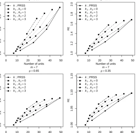
The traditional unbiased estimator of the population variance, based on SRS, is

ˆ

σ_SRS2 = _m−1₁Pm

i=1(Xi−X¯SRS)2. Stokes (1980) proposed an estimator of population variance on the basis of RSS, ˆσ2_RSS = _m−1₁Pm

i=1(Xi(i:m) − X¯RSS)2. This estimator is biased for small samples, and it is asymptotically unbiased. Suppose for given values ofmandk,X₁∗, X₂∗, , ..., X_m∗ represent a partial ranked set

(27)

1.4 Estimation of population median and variance 7 10 20 30 40 50 1.0 1.5 2.0 2.5 3.0 3.5 4.0 _{RSS k}₌₀ PRSS k=1 PRSS k=2 PRSS k=3 Number of units Relativ e Efficiency Normal(0,1) 10 20 30 40 50 1.0 1.5 2.0 2.5 3.0 3.5 4.0 _{RSS k}₌₀ PRSS k=1 PRSS k=2 PRSS k=3 Number of units Relativ e Efficiency Uniform(0,1) 10 20 30 40 50 1.0 1.5 2.0 2.5 3.0 3.5 4.0 _{RSS k}₌₀ PRSS k=1 PRSS k=2 PRSS k=3 Number of units Relativ e Efficiency Logistic(0,1) 10 20 30 40 50 1.0 1.5 2.0 2.5 3.0 3.5 4.0 _{RSS k}₌₀ PRSS k=1 PRSS k=2 PRSS k=3 Number of units Relativ e Efficiency Beta(6,6) 10 20 30 40 50 1.0 1.5 2.0 2.5 3.0 3.5 4.0 _{RSS k}₌₀ PRSS k=1 PRSS k=2 PRSS k=3 Number of units Relativ e Efficiency Exponential(1) 10 20 30 40 50 1 2 3 4 5 6 7 RSS k=0 PRSS k=1 PRSS k=2 PRSS k=3 Number of units Relativ e Efficiency Weibull(0.5,1) 10 20 30 40 50 1 2 3 4 5 RSS k=0 PRSS k=1 PRSS k=2 PRSS k=3 Number of units Relativ e Efficiency Lognormal(0,1) 10 20 30 40 50 1 2 3 4 5 6 RSS k=0 PRSS k=1 PRSS k=2 PRSS k=3 Number of units Relativ e Efficiency Gamma(0.5,2) 10 20 30 40 50 1.0 1.5 2.0 2.5 3.0 3.5 4.0 _{RSS k}₌₀ PRSS k=1 PRSS k=2 PRSS k=3 Number of units Relativ e Efficiency ρ =0.99 10 20 30 40 50 1.0 1.2 1.4 1.6 1.8 2.0 _{RSS k}₌₀ PRSS k=1 PRSS k=2 PRSS k=3 Number of units Relativ e Efficiency ρ =0.80 10 20 30 40 50 1.00 1.10 1.20 1.30 RSS k=0 PRSS k=1 PRSS k=2 PRSS k=3 Number of units Relativ e Efficiency ρ =0.50 10 20 30 40 50 1.00 1.01 1.02 1.03 1.04 1.05 RSS k=0 PRSS k=1 PRSS k=2 PRSS k=3 Number of units Relativ e Efficiency ρ =0.20

Figure 1.2: REs of PRSS with respect to SRS for estimating population median under perfect and imperfect rankings

sample of sizemfrom the parent population. Then, analogous to ˆσ2_RSS, the variance estimator under PRSS is ˆσ_PRSS2 = _m−1₁Pm

i=1(X ∗

i −X¯PRSS)2. The REs of ˆσ_PRSS2 and ˆσ_RSS2 with respect to ˆσ2_SRS, respectively, are given by

RE(ˆσ_PRSS2 ,σˆ2_SRS) = MSE(ˆσ

2 SRS)

MSE(ˆσ2_PRSS) and RE(ˆσ

2

RSS,ˆσSRS2 ) =MSE(ˆ

σ2_SRS) MSE(ˆσ2_RSS). The estimated MSE of any estimator, say ˆσ2J, is MSE(ˆσ2J) =_N1 PN

i₌₁(ˆσ2i,J−σ2)2, forJ = SRS, RSS, PRSS. On the basis of Figure 1.2, we can conclude that the PRSS median estimator is more efficient than SRS median estimator based on the same sample size. As the value of the coefficientkdecreases, the RE under PRSS increases. Under perfect and imperfect rankings, the PRSS estimator still performs better than the SRS estimator for all cases considered here. Furthermore, as the value ofρdecreases, the REs also decrease because of more errors in ranking and vice-versa.

(28)

10 20 30 40 50 0.5 1.0 1.5 2.0 2.5 _{RSS k}₌₀ PRSS k=1 PRSS k=2 PRSS k=3 Number of units Relativ e Efficiency Normal(0,1) 10 20 30 40 50 0.5 1.0 1.5 2.0 2.5 _{RSS k}₌₀ PRSS k=1 PRSS k=2 PRSS k=3 Number of units Relativ e Efficiency Uniform(0,1) 10 20 30 40 50 0.5 1.0 1.5 2.0 2.5 _{RSS k}₌₀ PRSS k=1 PRSS k=2 PRSS k=3 Number of units Relativ e Efficiency Logistic(0,1) 10 20 30 40 50 0.5 1.0 1.5 2.0 2.5 _{RSS k}₌₀ PRSS k=1 PRSS k=2 PRSS k=3 Number of units Relativ e Efficiency Beta(6,6) 10 20 30 40 50 1 2 3 4 RSS k_{PRSS k}=₌0₁ PRSS k=2 PRSS k=3 Number of units Relativ e Efficiency Exponential(1) 10 20 30 40 50 1 2 3 4 RSS k_{PRSS k}=₌0₁ PRSS k=2 PRSS k=3 Number of units Relativ e Efficiency Weibull(0.5,1) 10 20 30 40 50 1 2 3 4 RSS k_{PRSS k}=₌0₁ PRSS k=2 PRSS k=3 Number of units Relativ e Efficiency Lognormal(0,1) 10 20 30 40 50 1 2 3 4 RSS k_{PRSS k}=₌0₁ PRSS k=2 PRSS k=3 Number of units Relativ e Efficiency Gamma(0.5,2)

Figure 1.3: REs of PRSS with respect to SRS for estimating population variance under perfect and imperfect rankings

the proposed variance estimator is high as compared with the estimators based on SRS and RSS schemes. For symmetric populations, under RSS, as the number of units increase, this leads to the gain in RE of the estimator. On the other hand, the RE is a decreasing function of the number of units under PRSS for symmetric population. In variance estimation, PRSS is more economical than SRS and RSS. The variance estimator under PRSS uses less number of units and performs better than the other estimators. Therefore, in practice, for small samples, it is preferable to use PRSS variance estimator.

Generally, the optimum choice ofkdepends on the environment and experimenter. For instance, if the experimenter can rank all of sets with full confidence, then it is better to take k= 0. But when there are cost or time constraints or lack of units, then it is preferable to use PRSS with k >0. In case of mean estimation, if the underlying distribution is highly skewed, then it is preferable to apply the PRSS with k= 1 instead of using RSS method. Finally, in variance estimation with small samples,k= 1 is the optimal choice.

1.5

An application

A real data set is used to study the efficiency of the PRSS design in estimating the population mean, median and variance as compared with the SRS. The data consist of the diameter of conifer tree at breast height, say Y, and the height of the conifer tree, sayX. For more details about the data, see Platt et al. (1988). Table 1.1 contains the summary statistics of the trees data. Here, we are interested in estimating the mean, median and variation among the heights of the conifer trees population. The values of the samples sizes are m= 4,5,6,7 with different possible values of k. In order to select a ranked set sample of size m= 7, the experimenter needs to identify 49 conifer trees; but because of limited time or budget, it is difficult to apply

(29)

1.6 Concluding remarks 9

the RSS procedure. Suppose no more than 40 trees can be measured. In such situations, PRSS provides an opportunity to the PRSS(m, k) scheme, i.e., PRSS(7,1) with 37 units, PRSS(7,2) with 25 units and PRSS(7,3) with 13 units. One million replications were used to estimate the MSEs of the estimators under SRS, RSS and PRSS. The coefficient of skewness of the diameter is 0.884 and the skewness of height is 1.619. Therefore, these data are asymmetrically distributed.

Table 1.1: Summary statistics of 399 trees data

Variable Mean Median Variance Skewness Kurtosis

Diameter (Y)(cm) 20.84 14.5 310.11 0.884 −0.423

Height (X) (ft) 52.36 29 325.14 1.619 1.776

Correlation coefficient (ρ) 0.908

It is evident from Table 1.2 that the mean and median estimators based on PRSS are more efficient as compared with their competitors under SRS. As expected, the REs are generally high under perfect ranking as compared with imperfect ranking. For a fixed value of m, as the value ofk increases, the REs tend to decrease. It is of interest to note here that, for small samples, the PRSS variance estimator is more efficient than the variance estimators under SRS and RSS. Furthermore, PRSS uses less number of units as compared with the units required in RSS procedure, and at the same time, it provides more efficient estimates than RSS.

1.6

Concluding remarks

In this chapter, we proposed a PRSS design for estimating the population mean, median and variance. PRSS provides an unbiased estimator of the population mean when the underlying population is symmetric. On the basis of extensive Monte Carlo simulations, it was observed that for both perfect and imperfect rankings, the estimators under PRSS are more efficient than the estimators based on SRS. In the variance estimation, especially for small samples, PRSS provides efficient variance estimates than the estimates under SRS and RSS designs. Therefore, it is recommended to use PRSS design as an efficient alternative to SRS design in case of population mean, median and variance estimation.

This work can be extended to develop ratio and regression estimators of the population mean and median under PRSS. Also, the current work can be extended to multistage partial ranked set sampling design.

(30)

T able 1.2: Estimation of the p opulation mean, median and v ariance o f the study v ariable X under p erfect and imp erfect rankings Mean Median V ariance RSS PRSS PRSS PRSS RSS PRSS PRSS PRSS RSS PRS S PRSS PRSS Ranking k = 0 k = 1 k = 2 k = 3 k = 0 k = 1 k = 2 k = 3 k = 0 k = 1 k = 2 k = 3 m = 4 X 1.93229 1.40117 ——– ——– 2.35689 1.88827 ——– ——– 0.95619 1.28807 ——– ——– Y 1.76474 1.32658 ——– ——– 2.02863 1.70739 ——– ——– 0.94762 1.21507 ——– ——– m = 5 X 2.22719 1.52644 1.16415 ——– 3.01825 2.40034 1.47281 ——– 1.07035 1.30545 1.09905 ——– Y 1.96547 1.43816 1.14066 ——– 2.60930 2.16476 1.39176 ——– 1.02916 1.22735 1.08738 ——– m = 6 X 2.52027 1.62581 1.27675 ——– 3.53694 2.82148 1.96619 ——– 1.18465 1.29887 1.13812 ——– Y 2.14987 1.52776 1.24022 ——– 2.95560 2.50393 1.80554 ——– 1.10424 1.22805 1.12365 ——– m = 7 X 2.80720 1.71135 1.34462 1.12098 4.00582 3.22178 2.54038 1.43774 1.30096 1.28833 1.13252 1.05779 Y 2.32114 1.60863 1.30656 1.10899 3.38511 2.86422 2.28398 1.38009 1.17128 1.22848 1.12108 1.05496

(31)

Chapter 2

Mixed Ranked Set Sampling Design

This chapter appeared in:

Haq, A., Brown, J., Moltchanova, E., Al-Omari, A.I., 2014, Mixed ranked set sampling design, Journal of Applied Statistics, 41(10), 2141–2156.

The main focus of agricultural, ecological and environmental studies is to develop well-designed, cost-effective and efficient sampling designs. Ranked set sampling (RSS) is one method that leads to accomplish such objectives by incorporating expert knowledge to its advantage. In this chapter, we propose an efficient sampling scheme, named mixed RSS (MxRSS), for estimation of the population mean and median. The MxRSS scheme is a suitable mixture of both simple random sampling (SRS) and RSS schemes. The MxRSS scheme provides an unbiased estimator of the population mean, and its variance is always less than the variance of sample mean based on SRS. For both symmetric and asymmetric populations, the mean and median estimators based on SRS, partial RSS (PRSS) and MxRSS schemes are compared. It turns out that the mean and median estimates under MxRSS scheme are more precise than those based on SRS scheme. Moreover, when estimating the mean of symmetric and some asymmetric populations, the mean estimates under MxRSS scheme are found to be more efficient than the mean estimates with PRSS scheme. An application to real data is also provided to illustrate the implementation of the proposed sampling scheme.

2.1

Introduction

In biomedical, environmental and ecological studies, situations may arise where taking the actual measurement of the sample observation is difficult (e.g., costly, destructive, time-consuming) but ranking a small set of selected units is comparatively easy and reliable. Ranking may be visually with respect to the study variable or by any inexpensive method. For example, if the interest lies in estimating the average height of trees in a forest, then it is easy to rank a small set of selected trees with respect to their heights. As another example,

(32)

in animal and growth studies, ages of animals may need to be determined but aging an animal is costly and time-consuming. However, variables on the physical size of an animal that are highly correlated with age are cheap and easy to collect. In all such situations, the traditional ranked set sampling (RSS) scheme can be used to achieve observational economy. The RSS scheme incorporates inexpensive auxiliary information related to the variable of interest as a way of gathering additional information in order to rank the selected sampling units. This use of supplementary information helps in selecting more representative samples from the target population.

The RSS scheme was first introduced by McIntyre (1952) for estimating mean pasture and forage yields. The statistical theory of the RSS scheme was developed by Takahasi and Wakimoto (1968). They showed that the sample mean under RSS scheme is an unbiased estimator of the population mean, and it is more efficient than the sample mean based on simple random sampling (SRS). Dell and Clutter (1972) studied the effect of imperfect rankings on the performance of RSS-based mean estimator. For more details and real applications of RSS scheme, see Yu and Lam (1997), Mode et al. (1999), Al-Saleh and Al-Shrafat (2001), Al-Saleh and Al-Omari (2002), Chen and Wang (2004), Husby et al. (2005), Chen (2007), Wang et al. (2009), Ozturk (2011) and references cited therein.

Recently, Haq et al. (2013b) suggested partial RSS (PRSS) scheme for estimation of the population mean, median and variance. They showed that RSS is a special case of PRSS. The PRSS scheme becomes a suitable alternative to the RSS scheme when there is a shortage of experimental units, identification of units is costly and time-consuming, data arrives in different batches, etc. In such situations, it is beneficial to make use of PRSS scheme for efficient estimation of population parameters. The main disadvantage of PRSS scheme is that it lacks flexibility or the options to select partial ranked set samples are limited. Additionally, the PRSS scheme provides biased mean estimates when sampling from asymmetric populations.

In this chapter, we extend the work on PRSS scheme and propose a mixed RSS (MxRSS) scheme for estimation of the population mean and median. The MxRSS scheme provides plenty of options to the experimenter when selecting the sample from population. This helps in keeping the cost at an affordable level. We show that the mean estimates under MxRSS scheme are not only unbiased but also more precise than the mean estimates with SRS scheme. For symmetric and some asymmetric distributions, the mean estimates under MxRSS are found to be more efficient than the mean estimates based on PRSS.

The rest of the chapter is organized as follows: Section 2.2 contains brief details about RSS and PRSS schemes. Section 2.3 introduces MxRSS scheme for estimation of the population mean based on perfect and imperfect rankings. In this section, we also estimate the means of symmetric and asymmetric populations based on SRS, PRSS and MxRSS schemes. Estimation of the population median under the aforesaid sampling schemes is considered in Section 2.4. Section 2.5 provides the numerical results obtained from real data, and Section 2.6 summarizes the main findings.

(33)

2.2 Sampling schemes 13

2.2

Sampling schemes

In this section, we explain RSS and PRSS schemes for estimation of the population mean.

2.2.1

Ranked set sampling

The RSS scheme incorporates cheap quantitative or qualitative auxiliary information in order to obtain a more representative sample from the underlying population before the real and more expensive sampling is done. The RSS procedure is as follows: identifym2 units from the parent population. These units are then allocated tomsets, each of sizemunits. Without knowing the actual values, the units within each set are ranked in an increasing order of magnitude with respect to the study variable. The ranking can be done by employing expert knowledge or by using any concomitant variable that is highly correlated with the study variable. After ranking all sets, the smallest ranked unit is quantified from the first set. Similarly, the second smallest ranked unit is quantified from the second set, and the procedure continues until the largest ranked unit is quantified from the last set. This completes one cycle of a ranked set sample of sizem. The whole procedure can be repeatedrtimes to obtainrcycles of ranked set sample with total sample sizen=mr.

Let Y be the study variable with probability density functionfY(y) and cumulative distribution function FY(y), with meanµY and variance σY2. LetY1, Y2, ..., Yn represent a simple random sample of size ndrawn fromfY(y). The sample mean ¯Y_SRS= _n1P

n

i₌₁Yi is an unbiased estimator ofµY with varianceσ2Y/n, i.e., E( ¯Y_SRS) =µY and Var( ¯YSRS) =σ2Y/n.

Let (Y₁₁j, Y12j, ..., Y1mj),(Y21j, Y22j, ..., Y2mj), ...,(Ym1j, Ym2j, ..., Ymmj) be mindependent simple random samples each of size m for the jth cycle for j = 1,2, ..., r. Let (Yi_(1:m₎j, Yi_(2:m₎j, ..., Yi₍m_:m₎j) denote the order statistics of theith simple random sample (Yi1j, Yi2j, ..., Yimj) obtained in thejth cycle. Apply the RSS scheme to m samples, obtained in the jth cycle, to obtain a ranked set sample of sizem, denoted by Yi(i:m)j, i = 1,2, ..., mandj = 1,2, ..., r. Let ¯YRSS = 1n

Pr

j=1

Pm

i=1Yi(i:m)j be the sample mean based on a ranked set sample of size n. Takahasi and Wakimoto (1968) showed that ¯Y_RSS is also an unbiased estimator ofµY, and its variance is less than the variance of the ¯Y_SRS, i.e., Var( ¯Y_RSS) = _nm1 Pm_i₌₁σ_Y2₍_i_:_m₎= Var( ¯Y_SRS)−_nm1 Pm

i=1(µY(i:m)−µY)2. HereµY(i:m)andσY2(i:m)are the population mean and the population variance ofYi(i:m)j, respectively.

2.2.2

Partial ranked set sampling

Recently, Haq et al. (2013b) suggested another version of RSS, named PRSS, for estimation of the population mean, median and variance. The PRSS scheme is a mixture of both SRS and RSS schemes. This scheme requires less number of identified units than the RSS scheme when selecting a sample of sizen, thus reducing the total cost, time and expenditure that are involved in sampling.

The PRSS procedure is as follows: Define a constant ksuch thatk = [αm] for 0≤α <0.5. Here, [·]

represents the largest integer not greater thanαm. Firstly, select a simple random sample of size 2kfrom the target population. Identifym(m−2k) units from the target population, and allocate them intom−2k sets,

(34)

each of sizem units. Rank the units within each set with respect to the study variable or as aforementioned. Select the ith smallest ranked unit from theith set for i=k+ 1, ..., m−k. This completes one cycle of a partial ranked set sample of sizem. For a large sample, the whole process can be repeatedrtimes in order to obtain a partial ranked set sample of sizen.

Note that the PRSS scheme is equivalent to the RSS scheme whenk= 0. Givenk, the PRSS scheme requires nm−2k(n−r) identified units from the target population in order to select a sample of sizen.

The sample mean based on a partial ranked set sample of sizenis given by

¯ Y_PRSS= 1 n   r X j=1 k X i=1 Yij+ r X j=1 m−k X i=k+1 Yi(i:m)j+ r X j=1 m X i=m−k+1 Yij  , with variance Var( ¯Y_PRSS) = 2kσ 2 Y nm + 1 nm m−k X i=k+1 σ2_Y₍_i_:_m₎.

For symmetric populations, ¯Y_PRSSis an unbiased estimator ofµY, and it is conditionally better than ¯Y_SRS. For details see Haq et al. (2013b).

2.3

Proposed sampling scheme

In this section, we propose MxRSS scheme for efficient estimation of the population mean.

In some ecological and environmental field studies, the ranking or identification of the experimental units is costly or time-consuming. Therefore, it is difficult to apply the RSS scheme with full confidence. The PRSS scheme is an alternative option to the RSS scheme that helps in reducing the ranking cost, but it is also restricted to some choices ofk for eachm. The MxRSS scheme is a suitable mixture of both SRS and RSS schemes that offers more flexibility to the experimenter in selecting more representative samples from the target population in different ways. This not only helps in reducing the ranking cost, time and expenditure, but the estimates based on MxRSS scheme turn out to be more precise than the estimates with SRS and PRSS schemes.

A mixed ranked set sample of sizencan be selected based on the following steps:

Step 1: Select k₁(0≤k₁≤m) units from the target population based on SRS scheme.

Step 2: Let k₂ be a constant such that k₂= [β(m−k₁)] for 0≤β ≤0.5. Identify (m−k₁)(m−k₁−k₂) units from the target population, and partition them intom−k₁−k₂sets, each of sizem−k₁units. Without knowing the actual values, rank the units within each set with respect to the study variable or by any inexpensive method.

Step 3: Select the ith smallest ranked unit from the firstm−k₁−k₂ sets, fori= 1,2, ..., m−k₁−k₂. Also select the (m−k₁−i+ 1)th smallest ranked unit from the firstk₂ sets. This completes one cycle of a mixed ranked set sample of sizem.

(35)

2.3 Proposed sampling scheme 15

It is to be noted that both SRS and RSS methods are special cases of the MxRSS scheme. Fork₁ =m, MxRSS scheme is equivalent to the traditional SRS scheme. Similarly, fork₁=k₂= 0, MxRSS scheme is equivalent to the RSS scheme. The total number of units that are required to select a mixed ranked set sample of sizenarek₁r+r(m−k₁)(m−k₁−k₂).

2.3.1

Estimation of the population mean

The sample mean based on a mixed ranked set sample of size nis defined as

¯ Y_MxRSS= 1 n   r X j=1 k1 X i=1 Yij+ r X j=1 m−k1−k2 X i=1 Yi(i:m−k1)j+ r X j=1 k2 X i=1 Yi(m−k1−i+1:m−k1)j   with variance Var( ¯Y_MxRSS) = 1 nm k1σ 2 Y + m−k1−k2 X i₌₁ σ_Y2₍_i_:_m−k1₎+ k2 X i₌₁ σ_Y2₍_m−k1−i_+1:_m−k1₎ +2 k2 X 1≤i<m−k1−i+1 σY₍i,m−k1−i+1:m−k1)  . Lemma 1:

(i)Y¯_MxRSSis an unbiased estimator of the population meanµY.

(ii)For any population, we have Var( ¯Y_MxRSS)≤Var( ¯Y_SRS). Proof: (i) E( ¯Y_MxRSS) = r n k1 X i₌₁ µY + m−k1−k2 X i₌₁ µY₍i_:m−k1)+ k2 X i₌₁ µY₍m−k1−i+1:m−k1) ! , = 1 m{k1µY + (m−k1)µY}=µY,

using the fact thatPt

i=1µY(i:t)=tµY, see Takahasi and Wakimoto (1968).

(ii) Var( ¯Y_MxRSS) = 1 nm k1σ 2 Y + m−k1−k2 X i₌₁ σ2_Y₍_i_:_m−k 1)+ k2 X i₌₁ σ2_Y₍_m−k 1−i+1:m−k1) +2 k2 X 1≤i<m−k1−i+1 σY₍i,m−k1−i+1:m−k1)  , = 1 nm  k1σY2 + m−k1 X i=1 σ_Y2₍_i_:_m−k 1)+ 2 k2 X 1≤i<m−k1−i+1 σY(i,m−k1−i+1:m−k1)  ,

where σY(i,m−k1−i+1:m−k1) ≥ 0, i = 1,2, ..., k2, is the positive covariance between Yi(i:m−k1)j and Yi(m−k1−i+1:m−k1)j.

(36)

Following Al-Saleh and Al-Omari (2002), we can write m−k1 X i₌₁ σ2_Y₍_i_:_m−k1₎= (m−k₁)σ_Y2 −2 m−k1 X 1≤i<j σY₍i,j_:m−k1).

Then, it follows that Var( ¯Y_MxRSS) = σ 2 Y n − 2 nm   m−k1 X 1≤i<j σY₍i,j_:m−k1)− k2 X 1≤i<m−k1−i+1 σY₍i,m−k1−i+1:m−k1)  ≥0.

Note that the first term, Pm−k1

1≤i<jσY(i,j:m−k1)≥ 0, contains all positive covariance terms including those

terms being subtracted from it, i.e.,Pk2

1≤i<m−k1−i+1σY(i,m−k1−i+1:m−k1). Thus, overall their difference is a

positive quantity, which completes the proof.

For any population, the relative efficiency (RE) of ¯Y_MxRSSwith respect to ¯Y_SRS is given by

RE( ¯Y_MxRSS,Y¯_SRS) = Var( ¯YSRS) Var( ¯Y_MxRSS), = 1 1−_mσ22 Y Pm−k1

1≤i<jσY(i,j:m−k1)−Pk1≤i<m−k2 1−i+1σY(i,m−k1−i+1:m−k1)

,

which is independent ofr.

2.3.2

Imperfect ranking schemes

Sometimes, it is difficult for the experimenter to rank the experimental units with full confidence with respect to the study variable. Dell and Clutter (1972) showed that the sample mean based on imperfect ranking remains an unbiased estimator of population mean as long as the ranking is better than the random ordering of the experimental units. Stokes (1977) showed that it is possible to judge the ranks of the study variable with respect to the ranks of the concomitant variable, sayX, that is cheap and correlated with the study variable. The assumptions imposed by Stokes (1977) in developing the model for imperfect ranking are:

(i) the regression ofY onX is linear,

(ii) the underlying distribution of standardized variables, i.e., Y−µY σY and

X−µX

σX , is same.

These conditions can be easily met when both (Y, X) follow a bivariate normal distribution. The mathematical model suggested by Stokes (1977) for imperfect ranking is given by

Yi_[i_:m_]j=µY +ρ σY σX Xi₍i_:m₎j−µX +ξij, i= 1,2, ..., m, j= 1,2, ..., r,

whereµY andµX are the population means,σY andσX are the population standard deviations, ofY and X, respectively,ρis the correlation coefficient between Y andX. Here,Xi(i:m)j is theith order statistic corresponding to t