Unsupervised methods to discover events from spatio-temporal data

(1)

Unsupervised methods to discover events from

spatio-temporal data

A DISSERTATION

SUBMITTED TO THE FACULTY OF THE GRADUATE SCHOOL OF THE UNIVERSITY OF MINNESOTA

BY

Xi Chen

IN PARTIAL FULFILLMENT OF THE REQUIREMENTS FOR THE DEGREE OF

Doctor of Philosophy

Prof. Vipin Kumar, Advisor

(2)

c

Xi Chen 2017

(3)

Acknowledgements

First of all, I would like to thank my advisor, Professor Vipin Kumar, for his uncondi-tional help, advice, and support. He is the person that walked me into the data mining world. I learned tons of skills and knowledge from him, which build the technique foun-dation for my future career. In addition, he also taught me how to learn a new thing, how to solve a new problem, how to present a work, and how to collaborate with people from different backgrounds. These knowledge and experience helped me finish my PhD study very fruitfully. And even more important, I believe all the things that I learned from him are treasures that will be of great values in my entire career.

I also would like to thank two brilliant researchers, Dr. Shyam Boriah, and Pro-fessor James Faghmous. I worked with them in different stages of my PhD study. To me, they are not only very respectful collaborators, but more like my mentors that helped me finally grow up as an independent researcher. Next, I would like to thank the committee members, Professor Shashi Shekhar, Professor Arindam Banerjee, and Professor Snigdhansu Chatterjee. I could not finish my dissertation without their help. Furthermore, deep thanks also go to the undergraduate students that worked with me very closely in many research projects, especially Yuanshun Yao, Sichao Shi, and Robert Warmka. In addition, many thanks go to my labmates in University of Minnesota for the colorful and rewarding time that we spent together. The chatting, discussions, and arguing related to data mining questions that we have in the lab and the Espresso cafe is one of my most cherished memory.

Last but the most important, I want to thank my family, especially my parents, Guisen Chen and Yumin Cai, and my husband Chao Guo. Nothing can be achieved in my life without the support and unconditional love they provide. You were and will always be my heroes.

(4)

Dedication

To my father, Chen Guisen, and my mother, Cai Yumin.

(5)

Abstract

Unsupervised event detection in spatio-temporal data aims to autonomously identify when and/or where events occurred with little or no human supervision. It is an active field of research with notable applications in social, Earth, and medical sciences. While event detection has enjoyed tremendous success in many domains, it is still a challenging problem due to the vastness of data points, presence of noise and missing values, the heterogeneous nature of spatio-temporal signals, and the large variety of event types.

Unsupervised event detection is a broad and yet open research area. Instead of exploring every aspect in this area, this dissertation focuses on four novel algorithms that covers two types of important events in spatio-temporal data: change-points and moving regions.

The first algorithm in this dissertation is the Persistence-Consistency (PC) frame-work. It is a general framework that can increase the robustness of change-point de-tection algorithms to noise and outliers. The major advantage of the PC framework is that it can work with most modeling-based change-point detection algorithms and improve their performance without modifying the selected change-point detection algo-rithm. We use two real-world applications, forest fire detection using a satellite dataset and activity segmentation from a mobile health dataset, to test the effectiveness of this framework.

The second and third algorithms in this dissertation are proposed to detect a novel type of change point, which is named as contextual change points. While most existing change points more or less indicate that the time series is different from what it was before, a contextual change point typically suggests an event that causes the relationship of several time series changes. Each of these two algorithms introduces one type of contextual change point and also presents an algorithm to detect the corresponding type of change point. We demonstrate the unique capabilities of these approaches with two applications: event detection in stock market data and forest fire detection using remote sensing data.

(6)

ticular type of moving regions (or dynamic spatio-temporal patterns) in noisy, incom-plete, and heterogeneous data. This task faces two major challenges: First, the regions (or clusters) are dynamic and may change in size, shape, and statistical properties over time. Second, numerous spatio-temporal data are incomplete, noisy, heterogeneous, and highly variable (over space and time). Our proposed approach fully utilizes the spatial contiguity and temporal similarity in the spatio-temporal data and, hence, can address the above two challenges. We demonstrate the performance of the proposed method on a real-world application of monitoring in-land water bodies on a global scale.

(7)

List of Tables

2.1 The confusion matrix for the fire detection experiment. . . 33 6.1 The summary of the proposed algorithms in this dissertation. . . 99

(11)

List of Figures

1.1 The taxonomy of events in spatio-temporal data. . . 2 1.2 Examples of spatial outliers and global outliers. . . 3 1.3 Hotspots in the gun crime incidents data in Portland between 2009 to 2013. 4 1.4 Two temporal outliers in a time-series data. . . 5 1.5 An example of an anomalous sub-sequence. . . 6 1.6 Examples of modeling-based time-series change points. . . 7 1.7 A raster spatio-temporal dataset typically is a three dimensional data cube. 8 1.8 An example of a moving region. . . 8 1.9 Examples of contextual time-series change points. . . 10 2.1 Examples of change points that can be detected by modeling-based

meth-ods. . . 13 2.2 A periodic time series that experiences a change in expectation and its

corresponding anomaly scores. . . 16 2.3 A stationary time series that experiences a change in variance and its

corresponding anomaly scores. . . 17 2.4 The impact of outliers on modeling-based change-point detection methods. 18 2.5 The decay phenomenon in a change-score time series. . . 19 2.6 The impact of noise on modeling-based change-point detection methods. 20 2.7 The construction of the anomaly score matrix for a time series. . . 26 2.8 Examples of the anomaly score matrix for different time series. . . 27 2.9 Illustration of the change-score calculation method in the PC framework. 29 2.10 Example EVI time-series from two locations where forest fires occurred. 32 2.11 The precision and recall curves of the proposed PC framework against

the four baseline methods. . . 35

(12)

accelerometer data. . . 36 2.13 A segment of a chest-mounted accelerometer time series with the reported

change points and the adjusted change points. . . 37 2.14 The performance of the PC framework against two baselines on the

ac-tivity segmentation through chest-mounted accelerometer data. . . 38 3.1 The comparison between S-CTCs and traditional change points. . . 41 3.2 Temporal outliers and S-CTCs are different patterns. . . 45 3.3 Illustration of the multimodal problem in the proposed S-CTC detection

methods. . . 49 3.4 Comparison between the CUSUM method and the proposed S-CTC

de-tection method in the stock price data of Sprint Corporation. . . 52 3.5 The stock price data of Sprint Corporation and its DPG around the time

when a S-CTC occurs. . . 52 3.6 The top 9 S-CTCs detected from the S&P 500 dataset. . . 53 3.7 Two EVI time series. The left one is from a burned area, and the right

one is from a drought area. . . 54 3.8 Prototypical EVI signals for drought and forest fire events. . . 55 3.9 Precision and recall curves of the proposed S-CTC detection algorithm

and the V2Delta method in forest fire detection using remote sensing data. 56 3.10 Two examples that demonstrate the advantages of the proposed S-CTC

detection method for fires detection in the context of droughts. . . 57 3.11 A false positive of the S-CTC detection method in detecting forest fires

due to the small denominator in the TAD function. . . 58 3.12 The proposed S-CTC detection method may also detect other types of

events in addition to forest fires. The given time series contains a S-CTC that indicates a land cover type conversation instead of a forest fire. . . 59 4.1 G-CTCs include two types of events: group disbanding and group

forma-tion. . . 62 4.2 A set of EVI time series which disbands in August 2009 because of a

forest fire. . . 63

(13)

method is sensitive to the selection of the clustering method and the corresponding parameters. . . 75 4.4 The entropy distance function is not aware of distances among clusters,

and hence is not suitable to calculate G-CTC scores. . . 76 4.5 Running time of the original DBSCAN implementation and the two

op-timized implementations. . . 78 4.6 Four disbanding events in a EVI time-series dataset that are detected by

the proposed G-CTC detection method. They correspond to a forest fire occurred in August 2009. . . 79 4.7 A G-CTC event in the stock price data showing a change in the grouping

of REITs. The two Self-service Storage companies forked out from the general REIT context. . . 81 5.1 An example of a dynamic spatio-temporal cluster. . . 84 5.2 Examples of data challenges (noise and missing values) associated with

spatio-temporal data. The data represent a remotely-sensed “wetness index” to estimate surface wetness. . . 86 5.3 An example of data heterogeneity. The data represent a remotely-sensed

“wetness index” to estimate surface wetness. . . 87 5.4 The proposed four-step spatio-temporal clustering paradigm. . . 88 5.5 The steps of creating stables clusters from a spatio-temporal data using

ST-DBSCAN. . . 90 5.6 Core segments and their corresponding temporal profiles . . . 92 5.7 Illustrative example of layer based classifier . . . 94 5.8 Positions of the 166 lake regions used in evaluating the performance of

the proposed spatio-temporal clustering method. . . 96 5.9 The performance of the proposed spatio-temporal clustering algorithm

and the two baselines on the test 166 lakes. . . 96 5.10 The performance of the proposed spatio-temporal clustering algorithm

and the two baselines as a function of missing data. . . 97 5.11 The performance of the proposed spatio-temporal clustering algorithm

and the two baselines as a function of noise. . . 97

(14)

Chapter 1

Introduction

Spatio-temporal data are rapidly becoming ubiquitous thanks to affordable sensors and storage. These information-rich data have the potential to revolutionize diverse fields such as social, Earth, and medical sciences where there is a need to extract and un-derstand complex phenomena and their dynamics. Additionally, data in such scientific domains tend to be unlabelled since collecting data labels is often a time-consuming and labor-intensive operation. This highlights the importance of unsupervised methods in analysing spatio-temporal data.

Unsupervised event detection is an important problem that has enjoyed tremendous interest in the data mining community [3, 5, 18, 21, 45, 52, 54, 69, 71]. Yet, it is still a challenging problem in many applications due to the vastness of data points, presence of noise and missing values, the heterogeneous nature of spatio-temporal signals, and the large variety of event types. Designing event detection methods that can overcome all the above challenges is an ultimate and yet ambitious task. This dissertation is one step in this direction. It includes four algorithms, each of which solves a combination of these challenges under certain assumptions. I hope that introducing these methods to the data mining community will allow us to explore the real-world event detection problem in more depth and design a host of methods to analyze spatio-temporal data more efficiently and accurately.

(15)

1.1

Events in spatio-temporal data

Literally, an event is an occurrence of something that is important. Although event detection is considered as one of the major research tasks, there is no formal definition of events in the data mining community. In this dissertation, I consider events as either rarely occurring patterns (e.g., outliers or anomalous) or patterns that include changes (e.g., change-points in a time-series or moving regions).

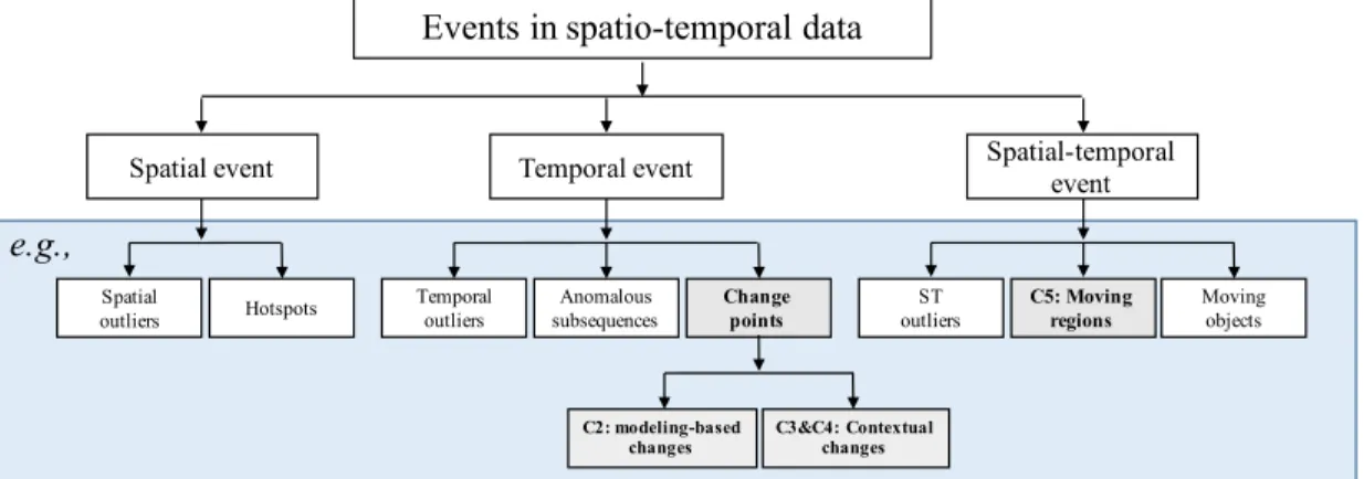
Spatio-temporal data typically contain three types of attributes: behavior attributes, temporal attributes, and spatial attributes. Theoretically, events can be defined by their behavior attributes only. However, most interesting events in spatio-temporal data are defined in the context of spatial and/or temporal information. I summarize events in temporal data into three categories: spatial events, temporal events, and spatio-temporal events. Figure 1.1 shows the taxonomy of events in spatio-spatio-temporal data. Figure 1.1 also provides several example events in each category (in the blue area). All the examples are commonly studied events and have been applied in real applications to solve critical problems. Among all types of events, this dissertation focuses only on modeling-based time-series points (Chapter 2), contextual time-series change-points (Chapter 3 and Chapter 4), and moving regions (Chapter 5). These three types of events are marked by grey blocks in Figure 1.1.

Events in spatio-temporal data

Spatial-temporal event Change points ST outliers Moving objects C5: Moving regions Temporal event Temporal outliers Spatial outliers Hotspots Spatial event C3&C4: Contextual changes C2: modeling-based changes 1 Anomalous subsequences e.g.,

(16)

1.1.1 Spatial events

Spatial events are data points with abnormal behavior attributes in the context of spatial attributes. Spatial outliers and hot-spots are two commonly seen spatial events.

Spatial outliers [18] are data points with abnormal behavior attributes compared with their spatial neighbors (i.e., data points that are spatially closed to the target data points). Figure 1.2 shows data points in a dataset. The x-axis and y-axis in Figure 1.2 are the two spatial attributes (i.e., the latitude and longitude) of the data points. The color of any point indicates the value of its behavior attribute. In other words, points with the same color have the same behavior attributes and points with different colors have different behavior attributes. The shapes of points are for illustration purposes and they are not related to data attributes. In Figure 1.2, the two rectangle points (one in red and the other in green) are spatial outliers. The red rectangle point is surrounded by blue points and the green rectangle point is surrounded by red points, which means that the two points have different behavior attributes compared with their spatial neighbors. Thus, the two rectangle points are spatial outliers.

Spatial outliers Longitude L at it ud e

The behavior attribute is 0 The behavior attribute is 1 The behavior attribute is 2 Global outliers

Figure 1.2: The x-axis and y-axis of the plot are the spatial attributes (i.e., the latitude and longitude). The color of a point indicates its behavior attribute. The two rectangle points are spatial outliers because they are surrounded by points with very different behavior attributes. The green rectangle point is also a global outlier with respect to the behavior attribute because it is the only green point in the dataset. The two triangle point are global outliers with respect to the spatial attributes since their spatial attributes are very different from all the other data points.

(17)

behavior attributes) that do not conform to the majority data. Figure 1.2 shows two types of global outliers: global outliers with respect to spatial attributes and global outliers with respect to behavior attributes. In detail, the blue triangle point and the red triangle point are global outliers with respect to spatial attributes since they are located very far away from the other points. In other words, their spatial attributes are very different from the majority of the points. The green rectangle point is a global outlier with respect to behavior attributes because its behavior attribute is different from all the other points (i.e., the green rectangle point is the only data point with green color). In contrast, in addition to the red rectangle point, there are many other red points in the plot. Hence, the red rectangle point is not a global outlier with respect to behavior attributes.

While global outliers indicate global extreme events (e.g., extremely low rainfall in the whole earth), spatial outliers are sensitive to locations (e.g., extremely low rainfall in Minnesota), and hence are critical in detecting regional events, such as local extreme meteorological events (e.g., tornadoes and hurricanes) and abnormal highway traffic patterns [20].

Figure 1.3: Hotspots (red regions) in the gun crime incidents data in Portland between 2009 to 2013. This example is from [2].

Hot-spots [11, 32, 68] are areas where the density of data (with a certain behavior attributes) is significantly higher than the other areas. Figure 1.3 shows the density map of gun crime incidents in Portland between 2009 and 2013 [2]. We can observe that

(18)

hotspots were dispersed throughout downtown and Northwest, Northeast, Southeast, and East Portland. Hot-spots have been widely used in analyzing social activities (e.g., crimes [15, 16, 73]) and biodiversity (e.g., the distribution of a certain species) [43, 74].

1.1.2 Temporal events

Temporal events are defined by behavior attributes and temporal attributes. Tempo-ral outliers, anomalous sub-sequences, and change-points are three commonly studied temporal events. 0 10 20 30 40 50 60 70 80 90 100 Time -2 -1.5 -1 -0.5 0 0.5 1

The behavior attribute

Figure 1.4: Two temporal outliers (the red point and the green point) in a time-series data. The red point is not a global outlier, while the green point is a global outlier.

Temporal outliers are time-points that do not follow the general temporal trend of a time-series. Similar to spatial outliers, temporal outliers may not be global outliers. Figure 1.4 shows two temporal outliers (a red point and a green point) in a time-series data. The x-axis in the plot is the temporal attribute and the y-axis is the behavior attribute. We can observe that both the green point and the red point do not match the general time-series trend. Thus, they are two temporal outliers. Additionally, the behavior attribute of the green point is different from all the other time points. Hence, the green point is also a global outlier (with respect to the behavior attributes). The red point, in contrast, is not a global outlier since its behavior attribute is similar to the behavior attributes of many other time points. Temporal outliers are important in detecting events that are sensitive to time. For example, 0 oF is normal and not very harmful during winter in Minnesota. But 0 oF in late spring or early summer in the same location can significantly reduce the yield of crops. Similar applications can be found in many other domains such as traffic control [57] and fraud detection [18].

(19)

0 10 20 30 40 50 60 70 80 90 100 Time -1 -0.8 -0.6 -0.4 -0.2 0 0.2 0.4 0.6 0.8 1

The behavior attribute

Figure 1.5: An example of anomalous sub-sequence (red points).

An anomalous sub-sequence, which is also known as a collective anomaly [18, 19], is several consecutive time-points that form an abnormal temporal pattern. Figure 1.5 shows an anomalous sub-sequence (marked as red points) in a periodic time-series. Anomalous sub-sequences have been applied to clinic data as key patterns of certain diseases. For example, an anomalous sub-sequence in electrocardiography data may indicate a heart problem [62]. In addition, anomalous sub-sequences are also used in detecting Web-based attacks [18] and monitoring air transportation systems [12].

Change points are the times when the behavior of one or more time series changes. Many types of change points have been defined in literature. Modeling-based change points, or structural change points, is one of the most commonly used types of change points [5, 46, 47, 71, 72, 78, 83, 86, 88]. Roughly speaking, a modeling-based time-series change point is the time when a time-series starts to significantly deviate from its own historical data.

Figure 1.6 (a) and (b) show two examples of modeling-based change points. The time series in Figure 1.6 (a) represents the monthly deaths and serious injuries on UK roads between 1975 and 1985. This time series contains one change point, which is marked by a red vertical dot line. This change point matches the time when the seat-belt law was introduced. Figure 1.6 (b) shows the chest-mounted accelerometer data (the y-acceleration field) that was recorded from a user when he was asked to do different activities. Vertical green lines in the plot indicate change points in the time series. All the change points are the times when the user changed his activity.

(20)

1975 1976 1977 1978 1979 1980 1981 1982 1983 1984 1985 1000 1200 1400 1600 1800 2000 2200 2400 2600 2800 3000

(a) Monthly deaths and serious injuries in UK roads between 1975 to 1985. The change point (the red vertical dot line) matches the time when the seat-belt law was introduced.

0 2 4 6 8 10 12 14 16 x 104 2000 2200 2400 2600 2800 3000

Reported Change Point

(b) The y-acceleration field in a chest-mounted accelerometer time-series data. The change points (green vertical lines) are the times when the user changed his activity.

Figure 1.6: Examples of modeling-based time-series change points.

1.1.3 Spatio-temporal events

Spatio-temporal events are defined in the context of both spatial and temporal infor-mation. Spatial outliers, moving objects, and moving regions are three examples of spatio-temporal events.

Similar to the definitions of spatial outliers and temporal outliers, spatio-temporal outliers are data points with abnormal behavior attributes compared with their spatio-temporal neighbors [26, 53]. Identifying spatio-spatio-temporal outliers can lead to discovery of many interesting events such as local instability or deformation. For example, Jun et al. [50] detects faulty sensors as spatio-temporal outliers in the sensor network.

Most studies on moving objects aim to discover the trajectory patterns of objects whose spatial attributes (e.g., GPS signals) change with time [51, 58–60, 77]. Examples of studied objects include animals, human beings, and cars. Moving object clusters [77] is one major type of event in this research area. Typically, moving object clusters are groups of objects that travel together for an extended period of time [51, 58, 59]. Dis-covery of such clusters is critical in understanding animal behaviors, detecting climate events (e.g., hurricane tracks), and helping in vehicle controls.

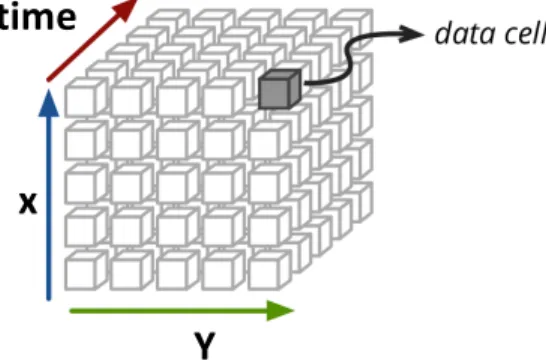
Typically, moving regions are defined in raster spatio-temporal data (e.g., earth-orbiting satellites, fMRI recordings, and surveillance videos). A raster spatio-temporal dataset is a three dimensional gridded data cube as shown in Figure 1.7. The three di-mensions consist of two dimensional spatial attributes (e.g., latitude and longitude) and

(21)

a one dimensional temporal attribute (i.e., date). Each data cell in the data cube con-tains one or multiple behavior attributes. For example, in surveillance videos, each data cell is a pixel in a certain time frame and it usually contains three behavior attributes (i.e., the R, G, and B values).

2

time

x

Y

Figure 1.7: A raster spatio-temporal dataset typically is a three dimensional data cube.

At any time-step, a region in a raster spatio-temporal dataset includes multiple spatially connected data cells that share similar behavior attributes. There is a moving region in the dataset when the position of the same region shifts or moves over time. Figure 1.8 shows an example of moving regions. In this example, red pixels in each time framework have similar behavior attributes in the SSH satellite dataset and hence each red area is a region. The regions in different time frames are located in different positions, but they indicate the same physical phenomenon (i.e., an ocean eddy [38]). Therefore, the red regions form a moving region.

!"#$%&'()*#+,-%#.%/,%0#123450,0

+,-%#0%/,%0#323450,0

!"#$%&'()%!("+!,&-(.!&$!/+(!0.#1.!223!$#4.5!

&4*0(!&$'(,($'($/.56!!7(!'(%")&1('!*$!*.0#)&/+4

8

!/+*/!&'($9:(%!

%(04($/%!#;!/+(!94(!%()&(%!*%%#"&*/('!<&/+!(''5!*"9=&/5>!/+($!

".?%/()%!%"#)('!,&-(.%!/#!;#)4!"#+()($/!%,*9*.!;(*/?)(%6!@+&%!*,,)#*"+!

&%!1(%/!%?&/('!/#!)(0&#$%!<+()(!(''&(%!*)(!&44#1&.(6

.637(8+%-6(/34#93&3#$,2,2:#;(/#.<343=4%#><%32#?))5#$(2,&(/,2:

@3-%0#A3:'-(B0

CDE

D#FBG%#.&54%0

C

D#H3/B2#$,&'34

C

D#.'53-#I(/,3'

C

D#.&%;32#F,%00

C

D#J3/0&%2#.&%,2'3B0%/

C

D#A/()%#H,G%=K

L

D#$,<'%4#)(0#.32&(0#$%0MB,&3

!

D#32)#H,6,2#JB-3/

C

AB!C$&=()%&/5!#;!D&$$(%#/*E!FB!G$%9/?/(!;#)!D*)&$(!H(%(*)"+>!I()0($>!J#)<*5E!8B!IK()L$(%!M($/)(!;#)!M.&4*/(!H(%(*)"+>!I()0($>!J#)<*5E!NB!K;*0+O"%6?4$6('?

P!%$*,%+#/!#;!%(*!%?);*"(!+(&0+/!*$#4*.5!'*/*!;#)!*!%&$0.(!'*5!&$!Q?$(!ARRS6 !T"(*$!+(&0+/!=*)&*1&.&/5!#$!/+(!UAVV!L4!%"*.(!&%!'#4&$*/('!15!(''5!*"9=&/56!

N"#O(34*#1#+/B%#.63&,(#8+%-6(/34#166/(3<'

M?))($/!4(/+#'%!%#.=(!/+(!%,*"(!*$'!94(!"#4,#$($/%!#;!/+(!(''5!'(/("9#$!,)#1.(4!&$!%(,*)*/(!

%/(,%>!<+()(!(*"+!#,()*/(%!&$!&0$#)*$"(!#;!/+(!#/+()W%!,()%,("9=(6!T?)!0#*.!&%!/#!'(:$(

P"#1<G2(Q4%):%-%2&0

R"#S%;%/%2<%0

E"#$%&'()*#9%&%<&,(2#,2#&'%#.63&,34#9(-3,2

9%&%<7(2#,2#&'%#063734#)(-3,2#

,)&#)&9X(%!&'($9;5&$0!(''5Y.&L(!

#1K("/%!&$!&$'&=&'?*.!94(!%/(,%6!M+(./#$!(/!*.6

F

!&/()*9=(.5!/+)(%+#.'%!

*$!223!&4*0(!/#!&'($9;5!"*$'&'*/(!"#$$("/('!"#4,#$($/%6!P$!#?/()!

.##,!/+($!?%(%!*!,)#-&4&/5!+(?)&%9"!/#!Z/)*"LW!/+(%(!#1K("/%!&$/#!

/(4,#)*..5!,()%&%/($/!(''&(%6!

C"#I3<G:/(B2)

[''&(%!*)(!)#/*9$0>!"#+()($/!1#'&(%!#;!<*/()!?1&\?&/#?%!

/+)#?0+#?/!/+(!0.#1*.!#"(*$6!@+(&)!$#$.&$(*)!$*/?)(!($*1.(%!

/+(4!/#!/)*$%,#)/!+(*/>!"+.#)#,+5..>!*$'!%*.&$&/5!;#)!

/+#?%*$'%!#;!4&.(%6![''&(%!*)(!')&=()%!#;!4*)&$(!("#%5%/(4!

'5$*4&"%!*$'!"#$/)&1?/(!/#!(-/)(4(!<(*/+()!(=($/%6

P/!)&0+/>!*!%*/(..&/(!&4*0(!'(,&"/%!*!/5,&"*.! 4(%#%"*.(!(''5!#]!/+(!%#?/+()$!9,!#;!P;)&"*6!! C,<(..&$0!;)#4!/+&%!(''5!)(%?./('!&$!*! ,+5/#,.*$L/#$!1.##4>!&$")(*%&$0!"+.#)#,+5..! "#$"($/)*9#$!*$'!&4,*)9$0!*!1)&0+/!0)(($! "#.#)6 ! P!"5".#$&"!(''5!"*?%('!/+(!'(*/+!#;!!/+(! SVVVY5(*)Y#.'!!D($/*<*&!)((;!&$!ARRS6! C,<(..&$0!!;)#4!/+(!(''5!"*?%('!*!4*%%&=(! ,+5/#,.*$L/#$!1.##4!/+*/!"#$%?4('!=&/*.! $?/)&($/%!*$'!*%,+5-&*/('!/+(!)((;6!A @+(!)#/*9#$!#;!/+(!<*/()!#$!*$!(''5W%! ,()&4(/()!"#))(%,#$'%!/#!*)(*!#;! *1$#)4*.!<*/()!!,)(%%?)(!/+*/!&%!=&%&1.(! &$!!%(*!%?);*"(!+(&0+/6 @+&%!)(%(*)"+!<*%!%?,,#)/('!&$!,*)/!15!*$!J2^!_)*'?*/(! H(%(*)"+!^(..#<%+&,>!*$!J2^!J#)'&"!H(%(*)"+!T,,#)/?$&/5! ^(..#<%+&,>!*$'!J2^!_)*$/!GG2YAVFRSAA6!P''&9#$*.! %?,,#)/!;)#4!/+(!J*9#$*.!H(%(*)"+!M#?$"&.!#;!J#)<*56! P""(%%!/#!"#4,?9$0!;*"&.&9(%!<*%!,)#=&'('!15!/+(! C$&=()%&/5!#;!D&$$(%#/*!2?,()"#4,?9$0!G$%9/?/(6

L"#T'344%2:%

D(%#%"*.(!(''&(%!*)(!'5$*4&"!$*/?)*.!,+($#4($*6!

2?""(%%;?.!'*/*!4&$&$0!#;!/+(%(!(=($/%!$("(%%&/*/(%!*""?)*/(!

0.#1*.!/)*"L&$0!#;!;(*/?)(%!/+*/>!<+&.(!,()%&%/($/!&$!94(>!

"#$%/*$/.5!*$'!?$,)('&"/*1.5!"+*$0(!&$!.#"*9#$!*$'!

*,,(*)*$"(6!@+(!'&`"?./5!#;!/+(!,)#1.(4!&%!"#4,#?$'('!15!

/+(!$*/?)*.!=*)&*1&.&/5!#;!/+(!<#).'W%!#"(*$%6

P/!.(a>!/+(!223!#;!*! ,&-(.!&$!/+(!J#)'&"!2(*! #=()!*!,()&#'!#;!FV! 5(*)%6!@+)((!,()&#'%!#;! (''5Y.&L(!*"9=&/5!+*=(! 1(($!&'($9:('6 ^#)!(*"+!94(!%/(,!!_">!/+(!,&-(.%! /+*/!*)(!&$!*$!(''5Y.&L(!%/*/(! *)(!".?%/()('!/#0(/+()!/#!;#)4! *!%,*9*..5!"#+()($/!;(*/?)(6 P/!.(a>!4#$/+.5! *$9"5".#$&"!(''5!"#?$/%! ;)#4!/+(!94(Y%()&(%Y 1*%('!*,,)#*"+!=()%?%! M+(./#$!(/!*.6!bM3AAcF!_@+(! '&]()($"(!&$!"#?$/%!&%>!&$! ,*)/>!'?(!/#!#?)!*1&.&/5!/#! /)*"L!%4*..()!(''&(%!&$!*$! (`"&($/!4*$$()! P1#=(>!*!%$*,%+#/!#;!%(*!%?);*"(!+(&0+/!*$#4*.5!'*/*!;#)!*!%&$0.(!'*5!&$! Q?$(!ARRS6!T"(*$!+(&0+/!=*)&*1&.&/5!#$!/+(!4(%#!bUAVV!L4c!%"*.(!&%! '#4&$*/('!15!(''5!*"9=&/56!F P/!.(a>!*$!(''5Y.&L(! ;(*/?)(!&%!+&0+.&0+/('!&$! %(\?($9*.!223!&4*0(%6 @+(!"?))($/!4(/+#'!&%!'(,($'($/!#$!4?.9,.(!,*)*4(/()%!/#!'(/()4&$(!/+(!".#%('! "#$/#?)%!#;!&$'&=&'?*.!(''&(%6!d(%,&/(!/+&%>!&/!&%!+&0+.5!!%?%"(,91.(!/#!0)#?,&$0!4?.9,.(>! 90+/.5!,*"L('!(''&(%!&$/#!*!%&$0.(!"#$$("/('!"#4,#$($/6!7(!&4,)#=(!/+&%!*,,)#*"+!15! &4,#%&$0!!*!.#<()!1#?$'!?,#$!/+(!)*9#!#;!/+(!%?);*"(!*)(*!#;!=*.&'!(''5Y.&L(!;(*/?)(%!/#! /+*/!#;!&/%!"#$=(-!+?..N_{6!@+&%!*''&9#$!)($'()%!%#4(!#/+()>!4#)(!"#4,?/*9#$*..5!} (-,($%&=(>!,*)*4(/()%!?$$("(%%*)56!D#)(#=()>!&/!0)(*/.5!&4,)#=(%!/+(!(`"*"5!#;!M+(./#$! (/!*.6W%!*,,)#*"+!&$!"#))("/.5!%(,*)*9$0!(''&(%!&$!".#%(!%,*9*.!,)#-&4&/56!I(.#<>!/+(!(]("/! #;!=*)&#?%!"#$=(-&/5!)*9#!.&4&/%!#$!/+(!%(,()*9#$!#;!&))(0?.*)!"#$/#?)%6

*$!*,,)#*"+!"#0$&X*$/!#;

1#/+!%,*"(!*$'!94(6!2?"+!*!

4(/+#'!<#?.'!%((!*..!

'&4($%&#$%!#;!/+(!'/!

%&4?./*$(#?%.5>!*$'!/+?%!

;?..5!(-,.#&/!(=()5!

'&4($%&#$!#;!/+(!223!'*/*!

"?1(6!@+(!223!#;!S-S!0)&'!

,#&$/%!&%!%+#<$!&$!/+(!:0?)(!

/#!/+(!.(a6!P!,(*L>!

"#))(%,#$'&$0!/#!*$!

*$9"5".#$&"!(''5>!4*5!1(!

#1%()=('!/)*=(.&$0!&$!/+(!

'&)("9#$!#;!/+(!)('!*))#<6!

eAf!H*+?.>!g6H6M6!(/!*.!bFVAVc6!hH#.(!#;!*!M5".#$&"![''5!&$! !!!!!!!!!!!/+(!SVVVYi(*)YT.'!D($/*<*&!M#)*.!H((;!d(*/+jk! ###########$%&'("%)(%#*)+#,%-&!%#.%)'")/#0%1%2'3#45556# eFf!M+(./#$!(/!*.!bFVAVc6!h_.#1*.!T1%()=*9#$!T;!J#$.&$(*)! !!!!!!!!!!!D(%#%"*.(![''&(%k6!72&/2%''#")#8(%*)&/2*9:;6# e8f!^*0+4#?%!(/!*.!bFVAFc6!hP!J#=(.!*$'!2"*.*1.(!2,*9#Y! !!!!!!!!!!!@(4,#)*.!@("+$&\?(!;#)!T"(*$![''5!D#$&/#)&$0k6! ###########72&(%%+")/'#&<#!:%#=>!:#???4#@&)<%2%)(%6# eNf!^*0+4#?%!(/!*.!bFVAFc6!h[''52"*$B!P!g+5%&"*..5! !!!!!!!!!!M#$%&%/($/!T"(*$![''5!D#$&/#)&$0!P,,.&"*9#$6k! ##########72&(%%+")/'#&<#!:%#=AB=#M&)<%2%)(%#&)#4)!%CC"/%)!#D*!*##### ##########E)+%2'!*)+")/6

Figure 1.8: An example of a moving region. The moving region (marked by red color pixels) is a moving eddy at five successive time-steps of SSH satellite data.

(22)

1.2

Summary of contributions

Discovery of events in spatio-temporal data is a wide open area. Instead of exploring every aspect in this domain, this dissertation includes four novel algorithms that cover two major types of events in spatio-temporal data: change-points and moving regions.

The first proposed algorithm is a Persistence Consistency (PC) framework. The PC framework is a solution to detect modeling-based change points in noisy time-series data. While modeling-based change-point detection methods have achieved tremendous success in many applications, they perform poorly when data are noisy and have out-liers. The PC framework enhances the performance of existing modeling-based methods when these data challenges exist. There are three contributions in this work. First, this work summarizes the common structure of most modeling-based change-point detection methods. Based on this common structure, it also introduces a four step approach to de-sign a modeling-based approach for a given application. Second, this work explains and demonstrates the negative impact of noise and outliers on a modeling-based approach. Finally, this work presents the PC framework. This PC framework can be combined with most modeling-based approaches to produce more accurate detection results when data are noisy and contain outliers.

The second and third algorithms in this dissertation are designed to detect contextual change points from time series. Contextual change points are a novel type of change point. While a modeling-based change point more or less indicates that the time series is different from what it was before, a contextual change point typically suggests an event that causes the relationship of several time series to change. This dissertation introduces two types of contextual change points: Singleton Contextual Time-series Change points (S-CTCs) and Group level Contextual Time-series Change points (G-CTCs). Roughly speaking, a S-CTC is the time when one time series starts to deviate from its “peer group” and a G-CTC is the time when a new peer group forms or an old peer group disbands. Here, we define the peer group as a group of highly correlated time series.

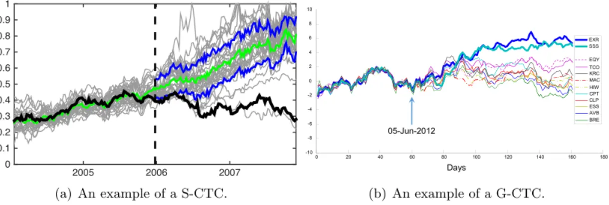
Figure 1.9 shows one example of S-CTC and one example of G-CTC. In Figure 1.9 (a), the stock price of Sprint Corporation (the black curve) behaved similarly to stock prices of several other companies (the grey curves) from year 2004 to year 2006. Hence, the grey time series formed a peer group of the black time series. The black time series

(23)

2005 2006 2007 0 0.1 0.2 0.3 0.4 0.5 0.6 0.7 0.8 0.9 1 (a) An example of a S-CTC. 0 20 40 60 80 100 120 140 160 180 -10 -8 -6 -4 -2 0 2 4 6 8 10 05-Jun-2012 AVB BRE CLP CPT EQY ESS EXR MAC SSS TCO HIW KRC Days (b) An example of a G-CTC.

Figure 1.9: Examples of contextual time-series change points.

began to deviate from its peer group in the beginning of year 2006. Therefore, there is a S-CTC occurred in Jan. 2006. We use blue lines for the 16 & 84 percentiles of all the grey time series after the change point, and a green line for the mean of the grey time series. In Figure 1.9 (b), several REITs stock price data had highly correlated behaviors before Jun. 5th, 2012, and hence they formed a peer group. The two self-service storage companies (one in dark blue and the other in light blue) began to fork out from the general REIT context, which led the whole group to split. Thus, Jun. 5th, 2012 is a G-CTC in the REITS stock price data.

As shown in Figure 1.9, contextual change points are useful patterns to discover events from non-stationary data, where the modeling-based change points are not suit-able. There are two major contributions in the work of detecting contextual changes. First, these two works introduce contextual time-series change points to the data mining community. Second, two algorithms are proposed. Each of them detects one particular type of contextual change point.

The last algorithm in this dissertation is to discover moving regions from a spatio-temporal dataset. This task faces two major challenges. First, the regions are dynamic and may change in size, shape, and statistical properties over time. Second, numer-ous spatio-temporal data are incomplete, noisy, heterogenenumer-ous, and highly variable (over space and time). The proposed algorithm is a new spatio-temporal data min-ing paradigm and can autonomously identify dynamic spatio-temporal clusters in the presence of the above data issues. The major contribution of this work is the proposed

(24)

paradigm. Compared with most existing methods, which either analyze data in space and then aggregate/associate over time, or analyze data over time and then smooth over space [30, 75], the proposed paradigm takes advantage of both spatial and tempo-ral auto-correlation. In addition, it utilizes knowledge from physical domains. Hence, it can discover moving regions in noisy, incomplete, and heterogeneous spatio-temporal data.

1.3

Thesis Overview

The remainder of this dissertation is organized in the following way. Chapter 2 presents the PC framework. The PC framework is a general framework that can increase the robustness of most modeling-based change-point detection methods to noise and outliers. Chapter 3 and Chapter 4 describe the two types of contextual change points and present the corresponding detection algorithms. Chapter 5 introduces the clustering paradigm that discovers a type of moving region in noisy, incomplete, and heterogeneous spatio-temporal data. Finally, Chapter 6 summarizes the whole dissertation and discusses potential research directions and applications of event detection in spatio-temporal data.

(25)

Chapter 2

The Persistence Consistency

(PC) framework:

A solution to detect change-points in noisy

time-series data using modeling-based methods

2.1

Motivation

Time-series change-point detection aims to autonomously identify time-steps where the behavior of a time-series significantly deviates from a predefined model. It is an active field of research with notable applications in finance [4], health [42], advertising [10], net-work security [41], and a host of other domains where data is presented as time-series. Figure 2.1 shows two examples of change-points (the red vertical lines) in a remote sensing time-series (left) and an automotive accident time-series (right). As the number of time-series continues to grow, there is an increasing need for autonomous change point detection and reporting methods. One common class of change-point detection algorithms relies on time-series models to define change-points. These modeling-based methods tend to be ad hoc, where each method is specifically tailored to the target ap-plication and deep domain expertise is required. While these methods are specialized, they share the common characteristic that they perform poorly when the data are noisy

(26)

2001 2002 2003 2004 2005 2006 2007 2008 2009 2010 2011 0 0.2 0.4 0.6 0.8 1 (18−Feb−2000 to 19−Dec−2011) EVI

(a) The “greenness” index of a forest area in Northern California. A forest fire oc-curred in this location in 2008.

1975 1976 1977 1978 1979 1980 1981 1982 1983 1984 1985 1000 1200 1400 1600 1800 2000 2200 2400 2600 2800 3000

(b) Monthly deaths and serious injuries on UK roads between 1975 to 1985. A seat-belt law was introduced in 1983.

Figure 2.1: Examples of change points (red vertical lines) that can be detected by modeling-based methods.

or have outliers. We propose a general framework to make existing modeling-based change-point detection algorithms robust to noise and outliers, regardless of the under-lying change point detection algorithms used by the researcher. This general framework immediately improves existing methods without the need to change the existing algo-rithm.

2.2

Background

As the name suggests, modeling-based point detection methods detect change-points by modeling the given time series. In detail, these methods assume data in a time-series are generated from a time-series model. We call this model the underlying model of the given time-series. Typically, the underlying model is a stochastic function. A time-series, in most cases, follows one single underlying model. However, sometimes the underlying model of a time-series may alter from one function to the other. The time when the underlying model changes is named change-points. Modeling-based change-point detection methods are concerned with detecting these change-change-points. Examples of modeling-based change-point detection methods include BFAST [88], the cumulative sum (CUSUM) chart [71, 72], and many other algorithms [5, 46, 47, 78, 83, 86].

(27)

2.2.1 The common structure of most modeling-based change-point de-tection methods

While the existing methods are numerous, most modeling-based change-point detection algorithms share a similar algorithm structure as shown in Algorithm 2.11 . In detail, these modeling-based methods can be defined by a time-series model function and a change-score function. Their final outputs are usually a change-score time-series.

Algorithm 2.1: calAnomalyT S

Input: x: a time-series data;

f(·): a time-series model;

g(·): a change-score function;

Output: a, a change-score time series;

1 forany x_t∈xdo

2 x0=x(t−w, t−1));;

3 θˆ=est(θ|x0, f);;

4 at=g(ˆθ, xt);;

5 end

The time-series model function is a mathematical function with several unknown parameters. Most algorithms assume the underlying models of all time-series data are the same function with different parameters. With the input time-series model function, a modeling-based detection method learns an underlying model for each time-series independently (Line 3). The change-score function is to calculate a change-score for each time-point in the time-series. The change-score of a time-step measures how much the underlying model changes around that time-step. Most change-point detection methods keep all change-scores of a given time-series also as a time-series (Line 4). We name it the change-score time-series.

After obtaining a change-score time-series for each input time-series, an algorithm can report the final change-points. There are two commonly used methods. First, we can label all time-steps as change-points if their change-scores exceed a user-defined

1

Algorithm 2.1 is a pseudo-code that calculates the change-score time-series for a given time-series. This algorithm trains the time-series model using a sliding-window approach and hence is good when detecting multiple change-points from a single time-series. This pseudo-code has been commonly used in many modeling-based change-point detection methods [5, 47, 88].

(28)

threshold. Second, we can report k points totally from the dataset. The change-points are the k time-steps with the highest change-scores in a certain time duration.

Hundreds of modeling-based change-point detection methods exist in the literature mainly due to the special tailored time-series model and change-score function. In most cases, these two components are designed in an application-specific fashion to achieve the best performance. In other words, most modeling-based change-point detection methods have their own time-series model and change-score function and are only suitable for one or several applications.

2.2.2 The four steps in designing a modeling-based change-point

de-tection method

The common structure of existing modeling-based change-point detection methods also inspires insights on how to design a new method for a particular detection task. Design-ing a new modelDesign-ing-based method usually involves four steps: (i) choose an appropriate time-series model; (ii) design a change-score function that quantifies how “different” two time-series segments are (before and after a change-point)2 ; (iii) compute the change-scores for each time-point based on the chosen time-series model and anomaly-score function; and (iv) select a mechanism to report change-points. Next, we illustrate the four steps using two simple examples.

Case I: Detecting abrupt changes for periodic time-series

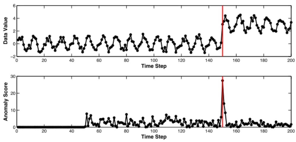
In case I, we aim to detect abrupt change-points in periodic time-series data. The top panel in Figure 2.2 shows one time-series (the black curve) and its change-point (the red line). As shown in Figure 2.2, data after the change-point have much higher values than data before the change-point. The given change occurs suddenly and dramatically. We name this type of changeabrupt changes. Here, we design a simple abrupt change-point detection method using the above mentioned four steps.

First, we choose an appropriate time-series model. Given the regular periodicity in the data, we choose the most simple seasonal ARIMA model [47]:

xt=αtxt−1+βtxt−p+e

2

Sometimes, the change-score may integrate anomaly-scores from multiple time-steps to enhance change events from random noise and/or outliers.

(29)

0 20 40 60 80 100 120 140 160 180 200 −2 0 2 4 6 Time Step Data Value 0 20 40 60 80 100 120 140 160 180 200 0 10 20 30 Time Step Anomaly Score

Figure 2.2: A periodic time series (on the top panel) that changes around the red line and its corresponding anomaly scores.

where, xtis the observation of the given time-seriesxat time-stept;pis the periodicity

of x, which is 10 in our example; eis a random noise term; and αt and βt are the two

unknown parameters.

Second, we choose an score function. Since the time-points after the change-point are dramatically greater than the time-change-points before the change-change-point (as shown in the top panel of Figure 2.2), we measure the degree of a change by the difference between the observed and the predicted values, which is:

at=|xˆt−xt|=|αˆtxt−1+ ˆβtxt−p−xt|

where at is the change-score of xt; ˆxt is the predicted observation; and ˆαt and ˆβt are

the two estimated parameters.

Next, we compute the change-score for each time-step. To obtain change-scores, we need to estimate ˆαt and ˆβtfor each time-stepxt. Here, we use a sliding window method

as shown in Algorithm 2.1 and set w to 50. The bottom panel of Figure 2.2 is the change-score time-series of the given example.

Finally, we report the change-points. Here, we use a threshold (e.g., 15) to report the event. For a more complex problem, we can train the threshold using a training set.

(30)

Case II: Detecting changes in variance for a stationary time-series

In case II, we need to detect changes in variance for a stationary time-series. Figure 2.3 shows one time-series (the black curve) and its two change-points (red vertical lines). We design a modeling-based change-point detection method also using the four steps.

0 20 40 60 80 100 120 140 160 180 200 −10 −5 0 5 10 Time Step Data Value 0 20 40 60 80 100 120 140 160 180 200 0 1 2 3 Time Step Anomaly Score

Figure 2.3: A stationary time series (top panel) that experiences a change in variance around the red line and its corresponding anomaly scores (bottom panel).

First, as shown in the top panel in Figure 2.3, the time-series is stationary (i.e., its expectation and variance are almost constants) when no change occurs. Hence, we select the time-series model as:

xt=α+et

where, αis a constant value; andet is the noise term that follows a Normal distribution

N(0, σ2_t). In this model, α and σt are the two unknown parameters.

Second, the top panel in Figure 2.3 also shows that only the variance of the time-series changes around the change-points. The expectation remains same. Therefore, we decide to score this event using the differences in the variance.

at=|log(

σtb

σta

)|=|log(σtb)−log(σta)|

where, σtb is the time-series variance before time-step xt and σta is the variance after

(31)

Next, we compute the change-score for each time-step. We use 30 values to estimate a variance value. In other words, σtb is the variance of {xt−30,· · · , xt−1} and σta is

the variance of {xt+1,· · ·, xt+30}. The change-score time-series of the given example is

shown in the bottom panel of Figure 2.3.

Finally, we report the change-points. For the given example, we can report time-points with the highest two change-scores as the final change-time-points.

2.2.3 Challenges

The majority of work in this area has focused on applied problems. General solutions have been less studied. Thus, there are two major opportunities within this line of work. First, there is an opportunity to create autonomous (application-agnostic) change-point detection algorithms that take any type of time-series and return change-points. Second, there is an opportunity to develop general solutions to overcome common data quality problems such as noise and outliers. The first opportunity is our grand vision but will require significant innovations. Instead, we focus on the second opportunity of creating a framework to allow existing model-based change-point detection algorithms to overcome outliers and noise. We next highlight how these challenges affect existing methods.

Outliers

Outliers are rare and anomalous observations that are different from the overall popu-lation. They are not change-points. Typically, the underlying time-series model does not change from one function to the other when an outlier presents. Figure 2.4 shows a time-series with two outliers (the red points).

0 10 20 30 40 50 60 70 80 90 100 -15 -10 -5 0 5 10 A B C D

(32)

0 50 100 150 200 0 2 time series 0 50 100 150 200 0 2 anomaly score

Figure 2.5: The decay phenomenon in a change-score time series.

Outliers negatively affect modeling-based change-point detection algorithms in two aspects: (i) they can be detected as change-points due to their anomalous behaviors; and (ii) they bias parameter estimation of the time-series model, especially when esti-mating the parameters using least square methods. Figure 2.4 demonstrates these two impacts of outliers. The figure shows a time-series that contains both change-points and outliers. The change score of a time step is defined as the absolute difference between its observation and the mean of its previous 20 time-steps. The four points highlighted with green color dots have change-scores 0.32(A), 1.95(B), 2.88(C) and 0.58(D). If we delete outliers manually and re-compute the change-scores, they are 0.15(A), 1.95(B), 2.88(C) and 2.54(D). The scores of A and D when outliers are removed are significantly different from the ones with outliers. This shows that outliers impact change-point detection, which in turn (i) causes non-change points to have artificially high change-scores; and (ii) decreases the change-scores of real change-points.

Noise

Noise is a random signal provided by a meaningless or irrelevant resource(s). Typically, noise is mixed with “real” signals and causes the observed data to randomly deviate from their true value. It can be challenging to detect change-points from a noisy time-series. Common solutions include (i) preprocessing the data; and (ii) aggregating change-scores of several consecutive time-steps to assess the significance of a change event. However, both of these solutions have limited applicability. First, preprocessing methods (e.g.,

(33)

smoothing), have aggregation issues and may introduce extra false negatives. Second, change-score aggregation methods tend to use the area-under-the-curve as a measure of the significance of a change event. This can be misleading since change-scores tend to be high and then decay over time as shown in Figure 2.5. This fact makes the area-under-the-curve an unreliable metric.

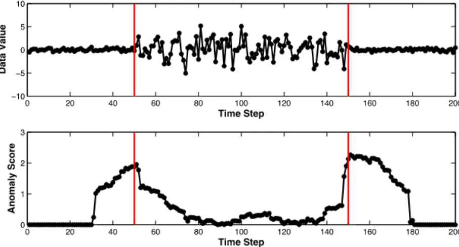
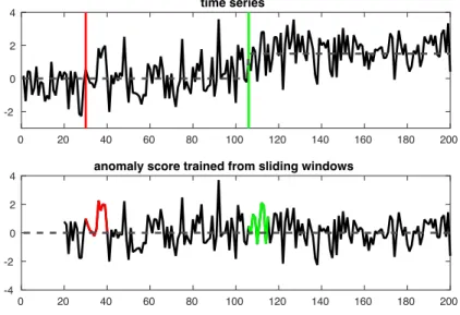
The top panel of Figure 2.6 shows a noisy time-series that changes around the green line. Its anomaly scores are shown in the bottom panel. The change-scores are calculated in the same way as the example shown in Figure 2.4. Note that the area under the curve of the real change-point (the green line) is smaller than the one caused by random noise (the red line).

0 20 40 60 80 100 120 140 160 180 200 -2 0 2 4 time series 0 20 40 60 80 100 120 140 160 180 200 -4 -2 0 2

4 anomaly score trained from sliding windows

0 20 40 60 80 100 120 140 160 180 200

-2 0 2

4 anomaly score trained from the first 20 time steps

Figure 2.6: The impact of noise on modeling-based change-point detection methods.

2.3

Proposed method

To improve the robustness of most existing modeling-based change-point detection methods to noise and outliers, we propose to: (i) utilize the central method to es-timate time-series models and calculate anomaly-scores and (ii) incorporate both the persistence and consistency properties to score the change events. Although the two proposed technologies can be used independently, we construct a framework that can use them together to achieve the best performance. In the following section, we first

(34)

introduce the central method and the concepts of persistence and consistency. Then, we present the proposed framework, which has been named the Persistence-Consistency (PC) framework.

2.3.1 The central method for anomaly-score estimation

As we discussed in Section 2.2, outliers, if they exist in the training data, can dra-matically reduce the accuracy of a time-series model estimation method and therefore negatively impact the final performance of the change-point detection algorithm. To address this challenge, we propose a central method to calculate anomaly-scores.

The central method is a random sampling technique. We show its pseudo-code as Algorithm 2.2. For comparison purposes, we also show Algorithm 2.1 from Section 2.2 on the right side. For the sake of simplicity, we use TS for time-series in all of the pseudo-codes.

Algorithm 2.2:calAnomalyCentral

Input: f(·), a TS model

g(·), an anomaly score function

x, a TS data

Output: a, An anomaly score TS

1 forany xt∈xdo 2 forr from1 toβ do 3 x0=sample(x(t−w, t−1)); 4 ˆθ=est(θ|x0, f); 5 temp_r=g(ˆθ, x_i) ; 6 end

7 a_t=med(temp₁,· · · , temp_β);

8 end

Algorithm 2.1: calAnomalyT S(·)

x, a TS data

Output: a, An anomaly score TS

1 forany xt∈xdo

2 x0=x(t−w, t−1)); 3 θˆ=est(θ|x0, f);

4 at=g(ˆθ, xt);

5 end

As introduced in Section 2.2, Algorithm 2.1 is one of the most commonly used meth-ods to generate an anomaly-score for each time-step. As shown in Line 2-3, Algorithm 2.1 uses all available data in the training window to estimate the time series model. When outliers occur in the training data, the estimated time-series model may dramati-cally differ from the true model. The proposed central method, on the other hand, does

(35)

not use all training data. Instead, it estimates one time-series model using a subset of the training data (Line 3 - 4 in Algorithm 2.2) and then calculates one anomaly score from the obtained model (Line 5 in Algorithm 2.2). We repeat this procedure multiple times (Line 2 - 6 in Algorithm 2.2). The final anomaly score is the median of all the obtained scores (Line 7 in Algorithm 2.2). The intuition behind the central method is to reduce the chance of including outliers in the training data.

The following lemma demonstrates the conditions under which anomaly scores cal-culated by the central method are not impacted by outliers at all. In many cases, even when the condition may not be fully satisfied, the central method can still largely increase the robustness of a change point detection method to outliers.

Lemma 2.1. Assume that the sampling rate is b, the outlier rate is o, and the times of the randomly sampling we do is n, then the probability that no outliers were used to estimate the parameters θ has the lower bound as below.

p(ˆθ= Θ|b, o)>(1−b−o 1−o )

on

where Θis the set of θ where no outliers are used in the estimation.

Proof. Letk=onand m=bn. The probability that no outliers were used to estimate

θ is p(ˆθ= Θ|b, o) = (n−k)! m!(n−m−k)! n! m!(n−m)! = (n−k)!(n−m)! (n−m−k)!n! When outliers are rare, we havek < m < n. Then,

p(θ= Θ|n, m, k) =(n−k)!(n−m)! (n−m−k)!n! =(n−m)(n−m−1)· · ·(n−m−k+ 1) n(n−1)· · ·(n−k+ 1) = k−1 Y i=0 n−m−i n−i

Also since 0< k < mand 0≤i≤k−1, we have

n−m−i n−i > n−m−k n−k = n−bn−on n−on = 1−b−o 1−o

(36)

Hence,

p(θ= Θ|n, m, k)>(1−b−o 1−o )

on

2.3.2 Persistence and Consistency

Persistence and consistency are two properties of change-points that we can use in a detection method to improve its detection accuracy when noise and outliers present in a dataset. More precisely, we can use the persistence property to distinguish change-points from outliers and the consistency property to enhance the performance of a detection method against noise.

Persistence is a characteristic that we use to avoid labeling outliers as change-points. We define an anomalous time-point (xt) to be persistent if many time-steps after xt

persistently differ from time-steps before xt. As discussed in Section 2.2, change-points

and outliers are two types of anomalous observations in a time series. The (underlying) time-series model is expected to change around a change-point but not around an outlier. Hence, we consider change-points as persistent anomalies since typically multiple time-steps after a change-point are significantly different from time-time-steps before the change point. In contrast, we define outliers as non-persistent anomalies since time-steps after an outlier typically follow the same time-series model as time-steps before the outlier.

Consistency is used to reduce false alerts due to random noise. We say an anomaly is consistent when the anomaly can be detected using multiple subsets of historical data. Most predictive modeling-based change-point detection methods use consecutive historical data to train the model (as shown in Line 2 in Algorithm 2.1). When data is very noisy, normal data may be assigned high anomaly scores occasionally. When change-points are very rare compared with normal points, a small fraction of false alerts can lead to a pool accuracy in the detection results. We use consistency to solve this problem. In detail, we assign multiple anomaly-scores to each time-step using different training data. We say an anomaly is consistent if all or most of its anomaly scores are high. Otherwise, the anomaly is inconsistent. Both change points and outliers are considered to be consistent. A normal data point, on the other hand, may have several high anomaly scores. But the probability that anomaly scores of a normal time-step are consistently high across different training sets is low.

(37)

2.3.3 The Persistence Consistency (PC) framework

The proposed Persistence-Consistency (PC) framework takes advantage of both the persistence and consistency properties. In addition, it is also very convenient to add the central method into the framework. Hence, the PC framework can dramatically increase the robustness of a given change point detection method to both noise and outliers. The PC framework can be applied to most modeling-based detection methods. Algorithm 2.3 shows the pseudo-code of the PC framework. This proposed frame-work has three types of inputs: (i) a time series data, which is denoted by a vector x; (ii) a change point detection method, which is characterized by a time-series modelf(·) and an anomaly-score function g(·); and (iii) a set of user-defined parameters Θ. Here, we assume that the selected time-series change-point detection method (i.e., f(·) and

g(·)) fits the application very well (i.e., the detection accuracy is very high) if no noise and outliers exist in the time-series data. The PC framework outputs a change-score for each time-step. We keep all the change-scores in a time-series (which is denoted by

y) and name the time-series as the change-score time-series.

Algorithm 2.3: The pseudo-code of the PC framework.

Input: x: a TS data;

f(·): a TS model;

g(·): an anomaly-score method; Θ: user defined parameters;

Output: y: a change score time series.

1 M =calAnomalyM atrix(x, f(·), g(·),Θ);

2 y=calChangeScoreT S(M,Θ);

There are two steps in the PC framework. The first step (Line 1 in Algorithm 2.3) is to calculate an anomaly-score matrix Mfor the given time-series datax. We name the first step anomaly-score matrix construction or function calAnomalyM atrix(·). The second step (Line 2 in Algorithm 2.3) is to generate the final change-score time-series from the obtained anomaly-score matrix. We call the second step change-score time-series generation or functioncalChangeScoreT S(·).

(38)

Anomaly-score matrix construction: calAnomalyM atrix(·)

Anomaly-score matrix is an internal data structure that we use to keep all the anomaly scores of the input time-series data. This novel data structure is the core component in the proposed PC framework. Algorithm 2.4 illustrates the construction process of the anomaly-score matrix for a given time-series x. Note that in Algorithm 2.4, we DO NOT include the central method for anomaly-score calculation. The most compre-hensive algorithm (i.e., the PC framework with the central method) is provided later in Algorithm 2.5. Again, we show Algorithm 2.1 on the right side of Algorithm 2.4 to highlight the differences between the construction of an anomaly-score matrix and an anomaly-score time-series.

Algorithm 2.4:calAnomalyM atrix

Input: x: a TS data;

f(·): a TS model;

g(·): an anomaly score function; Θ: user defined parameters;

Output: A: an anomaly score Matrix;

1 forany xt∈xdo

2 θˆ=est(θ|x(t−w, t−1), f); 3 fori fromt to the end do 4 At,i=g(ˆθ, xi); 5 end 6 end Algorithm 2.1: calAnomalyT S Input: x: a TS data; f(·): a TS model;

g(·): an anomaly score function; Θ: user defined parameters;

Output: a: an anomaly score TS;

1 foranyxt∈xdo

2 θˆ=est(θ|x(t−w, t−1), f);

3 at=g(ˆθ, xt);

4 end

The PC framework calculates anomaly-scores for multiple time-steps from a single estimated time-series model. In detail, for any qualified time stepxt, the PC framework

trains a time-series model using w data before it (i.e., time steps betweenxt−w andxt−1)

(Line 2 in Algorithm 2.4). This step is exactly the same as the selected change point detection method (Line 2 in Algorithm 2.1). Then, besides using the obtained model to estimate an anomaly score for time-step xt, the PC framework also estimates anomaly

scores for all time-steps after xt and keep all the obtained values in the corresponding

(39)

We repeat this procedure through a sliding window approach for all other qualified time-steps.

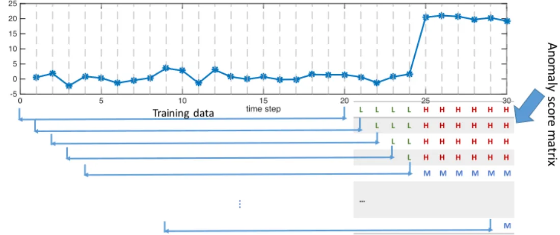
Figure 2.7 illustrates this process using an image to further help in understanding the construction process. The target time series is on the top of the image and its corresponding anomaly-score matrix is in the bottom right. Values in each row of the anomaly-score matrix are calculated using the same time series model. We mark the training window by a horizontal line on the left of that row and record the anomaly scores in the corresponding columns. For illustration purposes, instead of writing down the real anomaly score values, we use H (red), M (blue) and L (green) to indicate high anomaly scores, median anomaly scores, and low anomaly scores respectively in Figure 2.7. time step 0 5 10 15 20 25 30 -5 0 5 10 15 20 25 Training'data L L L L H H H H H H L L L H H H H H H L L H H H H H H L H H H H H H M M M M M M … M … An om aly 'sc ore 'm atr ix

Figure 2.7: The construction of the anomaly score matrix for a time series. The anomaly scores, in general, are continuous values. For the illustration purposes, we separate them into three categories and use H (red), M (blue) and L (green) to indicate high anomaly scores, median anomaly scores, and low anomaly scores respectively.

In anomaly-score matrix, as we discussed above, each time-series model generates multiple anomaly-scores for different time-steps. Simultaneously, each time-step gets multiple anomaly-scores. When we generate the anomaly-score matrix, we keep all the anomaly-scores for a single time-step in the same column (as shown in Figure 2.7). One interesting fact is that all the anomaly scores of a single time-step are obtained using different training sets. Such a novel data structure has several advantages.

(40)

time step 0 50 100 150 200 -5 0 5 10 15 time step 50 100 150 200 50 100 150 200 0 50 100 150 200

the time series

-5 0 5 10 15 time step 50 100 150 200

the change score matrix

50 100 150 200 time step 0 50 100 150 200 -20 0 20 time step 50 100 150 200 50 100 150 200

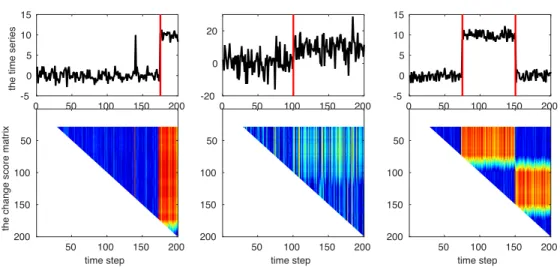
Figure 2.8: Examples of the anomaly score matrix for different time series.

First, outliers and change-points have easily discernible patterns in the anomaly-score matrix. The left panel in Figure 2.8 shows a time series (the top panel) and its corresponding anomaly-score matrix (the bottom panel). There are one outlier and one change-point in the time series. In the anomaly-score matrix, we use red for high anomaly-score values and blue for low values. Change-points have the persistence prop-erty and hence there is a patch of high anomaly scores (orange color) after the change point. In contrast, outliers are non-persistent anomalies and hence an outlier is shown in an anomaly-score matrix as one column of high values.

Second, the anomaly-score matrix also enables us to robustly detect change-points in a noisy time-series. The middle panel in Figure 2.8 shows a noisy time-series (top panel) with its anomaly-score matrix (bottom panel). Although the time-series is so noisy that any single anomaly-score (each cell in the matrix) is not strong enough to make a decision, we can still observe a patch with relatively high anomaly scores right after the change-point. This increases our ability to identify change-points in highly variable data.

Finally, the anomaly-score matrix allows us to easily identify multiple change-points in a single time-series. The right panel in Figure 2.8 shows a time-series with two change-points (top panel) and its anomaly-score matrix (bottom panel). We can clearly identify the two change-points as the time-steps preceding the high anomaly-score blocks in the bottom panel.

(41)

While Algorithm 2.4 has many advantages as we discussed above, the anomaly-score matrix itself still cannot reduce the negative impact of outliers on model estimation. To overcome this challenge, we need to incorporate the central method in the algorithm. Algorithm 2.5 is a more comprehensive algorithm that calculates the anomaly-score matrix using the central method.

Algorithm 2.5: calAnomalyM atrixCentral

x, a TS data

Θ: User defined parameters;

Output: A, An anomaly score Matrix

1 forany xt∈xdo

2 forr from 1 toβ do

3 x0 =sample(x(t−w, t−1));

4 θˆ=est(θ|x0, f);

5 fori from tto the end do

6 B_r,i =g(ˆθ, x_i) ;

7 end

8 end

9 fori fromt to the end do

10 A_t,i =med(B₁_,i,· · · ,B_β,i);

11 end

12 end

Change-score time-series calculation: calChangeScoreT S(·)

A change-point can be observed from an anomaly-score matrix as the boundary of a low anomaly score triangle block on the left and a high anomaly-score rectangle block on the right. When only one single change occurs in a time-series, as shown in the first two plots in Figure 2.8, the change-point is the column where the matrix is partitioned into the two most contrasting “sub-matrices”. However, when there are multiple change-points, as shown in the right panel in Figure 2.8, scoring change-points becomes a non-trivial

(42)

problem.

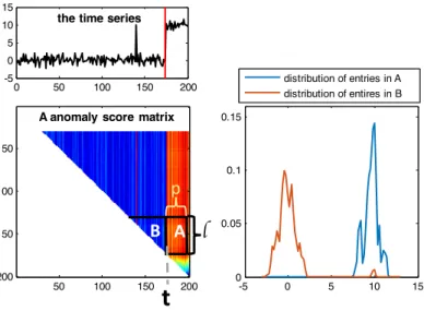
We use Figure 2.9 to illustrate the method we use to calculate change-scores. The detailed psedo-code is shown in Algorithm 2.6. The left panel in Figure 2.9 shows a time-series and its anomaly-score matrix. To account for multiple change events, we use a sliding window approach. We adopt Matlab notation for matrices. Let M(i1 :

i2, j1 : j2) be the sub-block in a matrix M that starts at the ith1 row and ends with

the ith₂ row, and starts at the j₁th column and ends with the j₂th column. Using this notation, we define Bt (the reference area of time stept) as the upper triangular part

of M(t−c:t−1, t−c:t−1) and At(the test area of time step t) as the sub-matrix

M(t−c:t−1, t+ 1 :t+p), wherep and care the parameters that control the size of the reference area and the test area.

0 50 100 150 200 -5 0 5 10 15

the time series

A anomaly score matrix

50 100 150 200 50 100 150 200 -5 0 5 10 15 0 0.05 0.1 0.15 distribution of entries in A distribution of entires in B A B

t

p l

Figure 2.9: Illustration of the change-score calculation method. The left: an illustrative example of how we report change events from an anomaly score matrix. The right: the distribution of entries in sub-matrix A and sub-matrix B. The change points can be detected as the column that maximizes the difference between the two distributions.

This proposed scoring method allows us to easily combine consistency and persis-tence properties. First, the length of both the reference area and the test area indicates theconsistency of an anomaly event – that is, an anomaly, whether an outlier or a real change, has high anomaly-scores based on multiple training sets. We use parameter c

(43)

event – that is, how long does the time-series model remain different from a training period. We use parameterp to control it.

We can detect the change points as the time-steps