October 2007, Volume 21, Issue 4. http://www.jstatsoft.org/
Enjoy the Joy of Copulas: With a Package
copula
Jun Yan
University of Connecticut
Abstract
Copulas have become a popular tool in multivariate modeling successfully applied in many fields. A good open-source implementation of copulas is much needed for more practitioners to enjoy the joy of copulas. This article presents the design, features, and some implementation details of the Rpackagecopula. The package provides a carefully designed and easily extensible platform for multivariate modeling with copulas in R. S4
classes for most frequently used elliptical copulas and Archimedean copulas are imple-mented, with methods for density/distribution evaluation, random number generation, and graphical display. Fitting copula-based models with maximum likelihood method is provided as template examples. With the classes and methods in the package, the package can be easily extended by user-defined copulas and margins to solve problems.
Keywords: copula, multivariate analysis,R.
1. Introduction
Copulas have become a popular multivariate modeling tool in many fields where multivariate dependence is of interest and the usual multivariate normality is in question. In actuarial science, copulas are used in modeling dependent mortality and losses (Frees, Carriere, and Valdez 1996; Frees and Valdez 1998; Frees and Wang 2005). In finance, copulas are used in asset allocation, credit scoring, default risk modeling, derivative pricing, and risk man-agement (Bouy`e, Durrleman, Bikeghbali, Riboulet, and Roncalli 2000;Embrechts, Lindskog, and McNeil 2003; Cherubini, Luciano, and Vecchiato 2004). In biomedical studies, copulas are used in modeling correlated event times and competing risks (Wang and Wells 2000; Es-carela and Carri`ere 2003). In engineering, copulas are used in multivariate process control and hydrological modeling (Yan 2006;Genest and Favre 2007).
p-dimensional random vectorU on the unit cube, a copula C is
C(u1, . . . , up) = Pr(U1≤u1, . . . , Up ≤up). (1)
Combined with the fact that any continuous random variable can be transformed to be uni-form over (0,1) by its probability integral transformation, copulas can be used to provide multivariate dependence structure separately from the marginal distributions. Copulas first appeared in the probability metrics literature. LetF be ap-dimensional distribution function with margins F1, . . . , Fp. Sklar(1959) first showed that there exists ap-dimensional copula
C such that for allx in the domain ofF,
F(x1, . . . , xp) =C{F1(x1), . . . , Fp(xp)}. (2)
The last two decades, particularly the last 10 years, witnessed the spread of copulas in statis-tical modeling. Joe (1997) and Nelsen(1999) are the two comprehensive treatments on this topic. A frequently cited and widely accessible reference isGenest and MacKay(1986), titled “The Joy of Copulas”, which gives properties of an important family of copulas, Archimedean
copulas; see Section 2.
For the joy of copulas to be enjoyable by everyone in need, software implementation is impor-tant. Unfortunately, there are very few software packages available for copula-based modeling. One of the exceptions is the S+FinMetrics module (Insightful Corporation 2002) of S-PLUS
(Insightful Corporation 2005). For an array of commonly used copulas, the S+FinMetrics module provides functions to evaluate their density and distribution, generate random num-bers from them, and fit them for given data. These functionalities, however, are limited because only bivariate copulas are implemented. Furthermore, the software is commercial. It is desirable to have an open source platform for the development of copula methods and applications.
“Ris a free software environment for statistical computing and graphics” (RDevelopment Core Team 2007a). It runs on all platforms including Unix/Linux, Windows, and MacOS. Cutting-edge statistical developments are easily incorporated intoRby the mechanism of contributed packages with quality assurance (R Development Core Team 2007b). It provides excellent graphics and interfaces easily with lower level compiled code such as C/C++orFortran. An active developer-user interaction is available through the R-help mailing list. Hundreds of contributed packages are available and many existing functionalities, for example, the density and distribution functions of multivariate normal andtdistributions, can be used for copulas. Therefore, it is a natural choice to write an Rpackage for copulas.
The packagecopulais designed using the object-oriented features of theSlanguage (Chambers 1998). It is publicly available at the Comprehensive R Archive Network (CRAN, http:// CRAN.R-project.org/). The new S4-style classes are created for multi-dimensional elliptical copulas and Archimedean copulas. The extreme value copula class is implemented for the bivariate case. For each copula family, methods of density, distribution, and random number generator are implemented. For visualization purpose, methods of contour and perspective plots are provided for bivariate copulas. Maximum likelihood method for fitting copula-based models is also available and can be easily extended.
The rest of the article is organized as follows. Section 2 briefly presents the S4-style classes defined in the package. Section 3 describe methods for copula classes, including density,
distribution, random number generator, and graphics. Section4illustrates how to fit copula-based models to data. Section5discusses some numerical issues in the implementation of the package. Section6 concludes.
In the sequel, all Rcode demonstration assumes that the package has been loaded:
R> library("copula")
The required packages mvtnorm (Genz, Bretz, and Hothorn 2005), sn (Azzalini 2006), and scatterplot3d(Ligges and M¨achler 2003), if not already loaded, will too be loaded by this call. To make all the illustrations reproducible, we set the random seed:
R> set.seed(1)
2. Classes
Two main classes are defined in thecopula package: copula and mvdc. The copula class is for defining copulas, while the mvdcclass is for defining multivariate distributions via copula. 2.1. The copula class
Two most frequently used copula families are elliptical copulas and Archimedean copulas. The copula package has implemented virtual classes ellipCopula and archmCopula, both extending the virtual class copula. These virtual classes are designed to provide a flexible way to associate actual classes, that share some properties but have different representations (Chambers 1998, p. 292).
An elliptical copula is the copula corresponding to an elliptical distribution by the Sklar’s theorem. General discussion about elliptical distributions can be found in Fang, Kotz, and Ng(1990). LetF be the multivariate CDF of an elliptical distribution. LetFi be CDF of the
ith margin and Fi−1 be its inverse function (quantile function), i = 1, . . . , p. The elliptical copula determined byF is
C(u1, . . . , up) =F[F1−1(u1), . . . , Fp−1(up)]. (3)
Elliptical copulas have become very popular in finance and risk management because of their easy implementation. Convenience in obtaining conditional distributions is another advantage in using them for predicting (Frees and Wang 2005).
Actual elliptical copula classes implemented in the package are normalCopula for normal copula tCopulafort-copula, specified by multivariate normal and multivariatetdistribution. Both copulas has a dispersion matrix, inherited from the elliptical distributions, andt-copula has one more parameter, the degrees of freedom (df). Since copulas are invariant to monotonic transformation of the margins, the standardized dispersion matrix, or correlation matrix, determines the dependence structure. Commonly used dispersion structures are implemented: autoregressive of order 1 (ar1), exchangeable (ex), Toeplitz (toep), and unstructured (un). The corresponding correlation matrices are, for example, in the case of dimension p= 3,
1 ρ1 ρ21 ρ1 1 ρ1 ρ2 1 ρ1 1 , 1 ρ1 ρ1 ρ1 1 ρ1 ρ1 ρ1 1 , 1 ρ1 ρ2 ρ1 1 ρ1 ρ2 ρ1 1 , and 1 ρ1 ρ2 ρ1 1 ρ3 ρ2 ρ3 1 , (4)
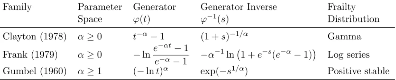
Family Parameter Generator Generator Inverse Frailty Space ϕ(t) ϕ−1(s) Distribution Clayton (1978) α≥0 t−α−1 (1 +s)−1/α Gamma Frank (1979) α≥0 −lne −αt−1 e−α−1 −α −1ln 1 +e−s(e−α−1) Log series Gumbel (1960) α≥1 (−lnt)α exp(−s1/α) Positive stable
Table 1: Summary of three One-Parameter (α) Archimedean Copulas for p >2.
whereρj’s are dispersion parameters. The following code creates a normalCopulaobject and
atCopula object, with self-explanatory arguments:
R> myCop.norm <- ellipCopula(family = "normal", dim = 3, dispstr = "ex",
+ param = 0.4)
R> myCop.t <- ellipCopula(family = "t", dim = 3, dispstr = "toep", + param = c(0.8, 0.5), df = 8)
These objects can be used to apply methods defined in Section3. An Archimedean copula is constructed through a generatorϕas
C(u1, . . . , up) =ϕ−1{ϕ(u1) +· · ·+ϕ(up)}, (5)
whereϕ−1is the inverse of the generatorϕ. In order for (5) to be a copula, the generator needs to be a p-monotonic function (see, for example, Nelsen 1999, Theorem 4.6.2). A generator uniquely (up to a scalar multiple) determines an Archimedean copula. Details of generators for various Archimedean copulas can be found inNelsen(1999).
Implemented Archimedean copula classes in the package are commonly used one-parameter families, such ascalytonCopula for Clayton copula (Clayton 1978),frankCopula for Frank copula (Frank 1979), andgumbelCopulafor Gumbel copula (Gumbel 1960). Constructors of these copulas are available. For example:
R> myCop.clayton <- archmCopula(family = "clayton", dim = 3, param = 2)
It is worth noting that Archimedean copulas with dimension 3 or higher only allows positive association. Negative association is allowed for bivariate Archimedean copulas. The three one-parameter multivariate Archimedean copulas (p > 2) implemented in the package are summarized in Table 1. The parameter value at the boundary of parameter space gives the independent copula after taking the limit. The generator inverse and frailty distribution are used in random number generation.
2.2. The mvdc class
The mvdc class is designed to construct multivariate distributions with given margins using copulas as in (2). This class is an actual class. It has three major components: copulaspecifies the copulaCin (2);marginsspecifies the names of the marginal distributionsF1, . . . , Fp; and
paramMargins is a list of list, each specifying the parameter values of the corresponding margin.
The following code creates amvdc object which represents a trivariate distribution with stan-dard normal margins and Clayton copula:
R> myMvd <- mvdc(copula = myCop.clayton, margins = c("norm", "norm", + "norm"), paramMargins = list(list(mean = 0, sd = 2), list(mean = 0, + sd = 1), list(mean = 0, sd = 2)))
Rprovides a comprehensive set of statistical distributionsRDevelopment Core Team(2007a), such as norm, t, gamma, lnorm, weibull, etc. They can be used to specify the margins. User-defined distributions can be used as long as the PDF, CDF, and quantile function of the distribution, with prefixd,p, andq, are available. For instance, if functionsdfancy,pfancy, andqfancyhave been supplied, then distributionfancycan be used in the margins. Of note is that these functions should be vectorized.
3. Methods
3.1. Distribution and densityThe method functions for distribution and density for a copula object are pcopula and
dcopula
For an elliptical copula, the distribution is (3). Evaluation of (3) needs implementation of the joint CDF of the elliptical distribution and univariate quantile functions for each margin. Differentiating (3) gives the density of an elliptical copula
c(u1, . . . , up) =
f[F1−1(u1), . . . , Fp−1(up)]
Qp
i=1fi[Fi−1(ui)]
, (6)
where f is the joint PDF of the elliptical distribution, and f1, . . . , fp are marginal density
functions. For example, after some algebra, the density of a Gaussian copula with dispersion matrix Σ is (Song 2000) c(u1, . . . , up|Σ) =|Σ|−1/2exp 1 2q >(I p−Σ−1)q , (7)
where q = (q1, . . . , qp)> with qi = Φ−1(ui) for i = 1, . . . , p, and Φ is the CDF of N(0,1).
Evaluation of (6) needs implementation of f and f1, . . . , fp in addition to the univariate
quantiles F1−1, . . . , Fp−1. Fortunately, the R package mvtnorm and sn provide F and f for multivariate normal and multivariate t. Other functions are available inRbase.
For an Archimedean copula, the distribution and density both depend on the generator func-tion and its inverse funcfunc-tion. These funcfunc-tions are defined for each Archimedean copula. The density of (5) is to be obtained by differentiating the distribution function, which, in many situations, can be very tedious. Symbolic differentiation is available through functionDinR
base and can be used to obtain CDF and PDF expressions. As the dimension p increases, however, the memory needed to do the symbolic differentiation to obtain PDF expression can go quickly beyond the available memory on a typical computer. Furthermore, because the expressions are not symbolically simplified, numerical problems may occur for particular
points in the support and for particular parameter values. In the current release, symbolic expressions are obtained fromMathematica and processed by functionderiv to generate al-gorithmic expressions before both are imported into R; see Section 5 for more details on numerical issues.
The method functions for distribution and density for a mvdc are pmvdc and dmvdc The distribution function is defined in (2). The density function is, by differentiating (2),
f(x1, . . . , xp) =c[F1(x1), . . . , Fp(xp)] p
Y
i=1
fi(xi) (8)
where cis the density of C, and f1, . . . , fp are marginal densities.
Example code to evaluate distribution and density will be given in the next subsection. 3.2. Random number generator
The random number generator method isrcopulafor acopulaobject andrmvdcfor anmvdc
object.
The random number generator of an elliptical copula is straightforward given a random num-ber generator of the corresponding elliptical distribution. The Sklar’s theorem implies that random numbers from a copula can be generated by transforming each margin of random numbers from a multivariate distribution with its probability integral transformation. The copulapackage provides generators for normal copula andt-copula using the random number generators for multivariate normal and multivariate tin packagemvtnorm.
Generating variables form a general copula can be done by iterative conditioning (Bouy`eet al. 2000). For some commonly used Archimedean copulas with p > 2, however, fast algorithm exits when the inverse generator functionϕ−1 is known to be the Laplace transform of some positive random variable (Marshall and Olkin 1988; Frees and Valdez 1998). This positive random variable is often referred to as frailty. Letγbe a realization of the frailty. Letv1, . . . , vp
be independent realizations of uniform variables over (0,1). Then ui = ϕ−1(−γ−1logvi),
i= 1, . . . , p, is a realization from the Archimedean copula with generatorϕ. This algorithm is very easy to implement and fast, given that a random number generator of the frailty is available. It is known that the frailty distribution for Clayton, Frank, and Gumbel copulas are gamma, log-series, and positive stable, respectively; see Table 1. Gamma variable generator is available in the Rbase. Algorithms for generating positive stable and log series variables can be found in Chambers, Mallows, and Stuck (1976) and Kemp (1981), respectively. In particular, the copula package uses a Fortran implementation of Nolan (2006), which is a revised version of Chambers et al. (1976), to generate positive stable variables. From the compound construction, this algorithm only allows positive association.
For bivariate Archimedean copulas (p= 2), negative association is allowed. Random number generator for bivariate Archimedean copulas are therefore separately implemented.
The following code illustrates the random number generation and evaluation of distribution and density for the copula objectmyCop.t created in Section2:
R> u <- rcopula(myCop.t, 4) R> u
[,1] [,2] [,3] [1,] 0.3508325 0.6165205 0.7459244 [2,] 0.3912433 0.2189641 0.2556491 [3,] 0.3925507 0.7579099 0.9157623 [4,] 0.9822296 0.9611676 0.8896553
R> cbind(dcopula(myCop.t, u), pcopula(myCop.t, u))
[,1] [,2] [1,] 2.265954 0.3081520 [2,] 3.493735 0.1359238 [3,] 1.878803 0.3777087 [4,] 31.481423 0.8771844
To generate random numbers from amvdcobject, one only needs to apply the quantile function to random numbers of the specified copula on each margin. The following code illustrates the random number generation and evaluation of distribution and density for themvdcobject
mymvd created in Section2:
R> x <- rmvdc(myMvd, 4) R> x [,1] [,2] [,3] [1,] 0.5330151 -0.06126913 2.17724731 [2,] -0.9815417 1.01855167 -0.05273936 [3,] 0.2210124 0.33882413 -0.48329446 [4,] -1.3613943 0.09657746 -1.09767362 R> cbind(dmvdc(myMvd, x), pmvdc(myMvd, x)) [,1] [,2] [1,] 0.01188019 0.3922578 [2,] 0.00589479 0.2686264 [3,] 0.02553551 0.3164067 [4,] 0.01971609 0.1842159 3.3. Graphics
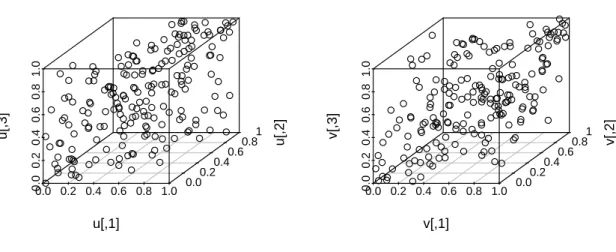
Graphics are important tools for in illustrating and presenting the results copula-based mod-eling. The 3D scatter plot from the packagescatterplot3dcan be used to show scatters. For example, the following code plots 200 random points from a trivariate normal copula and a trivariatet-copula in Figure 1.
R> par(mfrow = c(1, 2), mar = c(2, 2, 1, 1), oma = c(1, 1, 0, 0), + mgp = c(2, 1, 0))
R> u <- rcopula(myCop.norm, 200) R> scatterplot3d(u)
R> v <- rcopula(myCop.norm, 200) R> scatterplot3d(v)
0.0 0.2 0.4 0.6 0.8 1.00.0 0.2 0.4 0.6 0.8 1.0 0.00.2 0.40.6 0.81.0 u[,1] u[,2] u[,3] ● ● ● ● ● ● ● ● ● ● ● ● ● ● ● ● ● ● ● ● ● ● ● ● ● ● ● ● ● ● ● ● ● ● ● ● ● ● ● ● ● ● ● ● ● ● ● ● ● ● ● ● ● ● ● ● ● ● ● ● ● ● ● ● ● ● ● ● ● ● ● ● ● ● ● ● ● ● ● ● ● ● ● ● ● ● ● ● ● ● ● ● ● ● ● ● ● ● ● ● ● ● ● ● ● ● ● ● ● ● ● ● ● ● ● ● ● ● ● ● ● ● ● ● ● ● ● ● ● ● ● ● ● ● ● ● ● ● ● ● ● ● ● ● ● ● ● ● ● ● ● ● ● ● ● ● ● ● ● ● ● ● ● ● ● ● ● ● ● ● ● ● ● ● ● ● ● ● ● ● ● ● ● ● ● ● ● ● ● ● ● ● ● ● ● ● ● ● ● ● 0.0 0.2 0.4 0.6 0.8 1.00.0 0.2 0.4 0.6 0.8 1.0 0.00.2 0.40.6 0.81.0 v[,1] v[,2] v[,3] ● ● ● ● ● ● ● ● ● ● ● ● ● ● ● ● ● ● ● ● ● ● ● ● ● ● ● ● ● ● ● ● ● ● ● ● ● ● ● ● ● ● ● ● ● ● ● ● ● ● ● ● ● ● ● ● ● ● ● ● ● ● ● ● ● ● ● ● ● ● ● ● ● ● ● ● ● ● ● ● ● ● ● ● ● ● ● ● ● ● ● ● ● ● ● ● ● ● ●● ● ● ● ● ● ● ● ● ● ● ● ● ● ● ● ● ● ● ● ● ● ● ● ● ● ● ● ● ● ● ● ● ● ● ● ● ● ● ● ● ● ● ● ● ● ● ● ● ● ● ● ● ● ● ● ● ● ● ● ● ● ● ● ● ● ● ● ● ● ● ● ● ● ● ● ● ● ● ● ● ● ● ● ● ● ● ● ● ● ● ● ● ● ● ● ● ● ● ● ●
Figure 1: Scatter plots of random numbers from a normal copula and at-copula.
For both copula and mvdc objects, the copula package has implemented methods to draw perspective and contour plot for density and distribution. These method functions arepersp
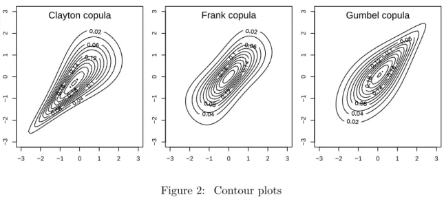
and contour. We illustrate the usage of contour for mvdc objects. The following code plots the density contours of bivariate distributions defined with Clayton, Frank, and Gumbel copulas, all with both margins being standard normal:
R> myMvd1 <- mvdc(copula = archmCopula(family = "clayton", param = 2), + margins = c("norm", "norm"), paramMargins = list(list(mean = 0, + sd = 1), list(mean = 0, sd = 1)))
R> myMvd2 <- mvdc(copula = archmCopula(family = "frank", param = 5.736), + margins = c("norm", "norm"), paramMargins = list(list(mean = 0, + sd = 1), list(mean = 0, sd = 1)))
R> myMvd3 <- mvdc(copula = archmCopula(family = "gumbel", param = 2), + margins = c("norm", "norm"), paramMargins = list(list(mean = 0, + sd = 1), list(mean = 0, sd = 1)))
R> par(mfrow = c(1, 3), mar = c(2, 2, 1, 1), oma = c(1, 1, 0, 0), + mgp = c(2, 1, 0))
R> contour(myMvd1, dmvdc, xlim = c(-3, 3), ylim = c(-3, 3)) R> contour(myMvd2, dmvdc, xlim = c(-3, 3), ylim = c(-3, 3)) R> contour(myMvd3, dmvdc, xlim = c(-3, 3), ylim = c(-3, 3))
The contour plots are shown in Figure2. Note that the parameters of the copulas are chosen such that the Kendall’sτ for all three distributions are 0.5.
The persp method can be called similarly. The first argument in these two calls are the signature that determines which method to call. It should be either a copula object or a
mvdc object. The second argument specifies the function for which the plots are to drawn, that is, PDF or CDF.
−3 −2 −1 0 1 2 3 −3 −2 −1 0 1 2 3 Clayton copula −3 −2 −1 0 1 2 3 −3 −2 −1 0 1 2 3 Frank copula −3 −2 −1 0 1 2 3 −3 −2 −1 0 1 2 3 Gumbel copula
Figure 2: Contour plots
4. Fit a copula model
With density functions for copulaandmvdc objects available, one can easily fit copula-based models with the maximum likelihood method. The package provides functionsloglikCopula
and loglikMvdc to evaluate the loglikelihood of the data under the specified copula model. These functions can be passed to an optimizer to obtain the maximum likelihood estimate. The package provides functions fitCopula and fitMvdc to carry out the estimation and report the results.
Suppose that we observe n indepent realizations from a multivariate distribution, {(Xi1, . . . , Xip)> : i = 1, . . . , n}. Suppose that the multivariate distribution is specified by
p margins with CDF Fi and PDF fi, i = 1, . . . , p, and a copula with density c. Let β be
the vector of marginal parameters and α be the vector of copula parameters. The parameter vector to be estimated is θ= (β>, α>)>. The loglikelihood function is
l(θ) = n X i=1 logc{F1(Xi1;β), . . . , Fp(Xip;β);α}+ n X i=1 p X j=1 logfi(Xij;β). (9) The ML estimator of θ is ˆ θML= argmax θ∈Θ l(θ),
where Θ is the parameter space.
To illustrate, we generate a sample from a bivariate distribution with gamma margins and a normal copula:
R> myMvd <- mvdc(copula = ellipCopula(family = "normal", param = 0.5), + margins = c("gamma", "gamma"), paramMargins = list(list(shape = 2, + scale = 1), list(shape = 3, scale = 2)))
R> n <- 200
R> dat <- rmvdc(myMvd, n)
The parameters to be estimated consist of marginal parameters β = (2,1,3,2)> and copula parameter α= 0.5. The loglikelihood at the true parameter value is:
R> loglikMvdc(c(2, 1, 3, 2, 0.5), dat, myMvd)
[1] -781.1641
To obtain ˆθML, one implements the loglikelihood function l(θ) and feed it to an optimizer. The function fitMvdcis a wrapper to the optimization routineoptim inR. An initial search point is needed for optim. Simpel method of moments estimate will serve as initial point.
R> mm <- apply(dat, 2, mean) R> vv <- apply(dat, 2, var)
R> b1.0 <- c(mm[1]^2/vv[1], vv[1]/mm[1]) R> b2.0 <- c(mm[2]^2/vv[2], vv[2]/mm[2])
R> a.0 <- sin(cor(dat[, 1], dat[, 2], method = "kendall") * pi/2) R> start <- c(b1.0, b2.0, a.0)
R> fit <- fitMvdc(dat, myMvd, start = start,
+ optim.control = list(trace = TRUE, maxit = 2000))
The first three arguments of function fitMvdc are the data, the mvdc object, and a start-ing value. Control parameters to the optimizstart-ing routine can passed in through argument
optim.control. The starting values here are arbitarily chosen. In real problems, the starting values of marginal parameters can be chosen by fitting each margin separately. The result of the estimation is summarized as:
R> fit
The ML estimation is based on 200 observations. Margin 1 : Estimate Std. Error m1.shape 1.830479 0.1689802 m1.scale 1.037388 0.1100475 Margin 2 : Estimate Std. Error m2.shape 3.515646 0.3362403 m2.scale 1.628037 0.1672812 Copula: Estimate Std. Error rho.1 0.419909 0.05820196
The maximized loglikelihood is -777.327 The convergence code is 0
As the dimension p gets large, the number of parameters increases, and the optimization problem gets harder. Joe and Xu (1996) proposed a two-stage estimation method called inference functions for margins (IFM). The IFM method estimates the marginal parameters
β in a first step by ˆ βIFM = argmax β n X i=1 p X j=1 logfi(Xij;β), (10)
and then estimates the association parametersαgiven ˆβIFM by ˆ αIFM = argmax α n X i=1 logc F1(Xi1; ˆβIFM), . . . , Fp(Xip; ˆβIFM);α . (11)
When each marginal distribution Fi has its own parameters βi so that β = (β1>, . . . , βp>)>,
the first step consists of an ML estimation for each marginj = 1, . . . , p: ˆ βjIFM= argmax βj n X i=1 logfi(Xij;βj). (12)
In this case, each maximization task has a very small number of parameters, greatly reducing the computational difficulty. This approach is called the two-stage parametric ML method by Shih and Louis (1995) in a censored data setting. In our illustration, the method can be carried out with the functionfitCopula.
R> loglik.marg <- function(b, x) sum(dgamma(x, shape = b[1], scale = b[2],
+ log = TRUE))
R> ctrl <- list(fnscale = -1)
R> b1hat <- optim(b1.0, fn = loglik.marg, x = dat[, 1], control = ctrl)$par R> b2hat <- optim(b2.0, fn = loglik.marg, x = dat[, 2], control = ctrl)$par R> udat <- cbind(pgamma(dat[, 1], shape = b1hat[1], scale = b1hat[2]), + pgamma(dat[, 2], shape = b2hat[1], scale = b2hat[2]))
R> fit.ifl <- fitCopula(udat, myMvd@copula, start = a.0)
The estimate from the two stage is summarized as
R> c(b1hat, b2hat, fit.ifl@est)
[1] 1.8301906 1.0375602 3.5167486 1.6284508 0.4199346
R> fit.ifl
The ML estimation is based on 200 observations. Estimate Std. Error z value Pr(>|z|) rho.1 0.4199346 0.05368175 7.822671 5.107026e-15 The maximized loglikelihood is 19.41620
The convergence code is 0
Note that the IFM estimate is close to the ML estimate. The standard error of ˆαIFM is underestimated because the variation of ˆβIFM is not appropriately taken care of.
When consistent estimation of the dependence parameterα is important, it can be estimated with the canonical ML (CML) method without specifying the marginal distributions. This approach uses the empirical CDF of each marginal distribution to transform the observations (Xi1, . . . , Xip)>into pseudo-observations with uniform margins (Ui1, . . . , Uip)> and then
esti-mates α as ˆ αCML= argmax α n X i=1 logc(Ui1, . . . , Uip;α). (13)
R> eu <- cbind((rank(dat[, 1]) - 0.5)/n, (rank(dat[, 2]) - 0.5)/n) R> fit.cml <- fitCopula(eu, myMvd@copula, start = a.0)
R> fit.cml
The ML estimation is based on 200 observations. Estimate Std. Error z value Pr(>|z|) rho.1 0.4304444 0.05311327 8.104272 4.440892e-16 The maximized loglikelihood is 20.29229
The convergence code is 0
The CML estimate ˆαCMLis noticeably different from ˆαMLand ˆαIFM. It has the advantage of not relying on marginal specifications.
Maximum likelihood estimation of copula-based models can be easily extended to solve more complicated problems. For example, when covariates are to be incorporated into the margins, all one needs to do is to write the loglikelihood function (9), which is the summation of the loglikelihood of the copula and the the loglikelihood of all the margins. Then, maximum likelihood estimates can be obtained by feeding the loglikelihood function to an optimizer. Example code for incorporating covariates into the margins is presented in the Appendix where two margins are modeled by gamma regression and log-normal regression, respectively. Covariates can also be incorporated into copula parameters in a similar fashion.
5. Numerical issues
The accuracy of the implemented functions is important for a user to feel comfortable using the package. Several numerical issues are encountered in the development of packagecopula: distribution/density evaluation, limits in parameter space, and constrained optimization. Al-though these issues are not yet elegantly solved in the package, they are worth bringing up for developers to seek for better solutions and for users to be aware of the potential limitations. Numerical issues in CDF/PDF evaluation mostly arise near or on the boundary of the support of copulas. Evaluation of CDFs is important in extreme value analysis because both lower and upper tail dependence indices are defined as the limits of CDFs in extreme values (Joe 1997, p.33). For example, the lower tail dependence index of a bivariate copula is λL =
limu→0Pr(U1 ≤u|U2 ≤u) = limu→0C(u, u)/u. Evaluation of PDFs is essential in likelihood based inferences. We focus our discussion on the numerical issues in PDF evaluation.
For an Archimedean copula, the PDF can be obtained in theory by differentiating the CDF, which is constructed from the generator function and its inverse function. Unfortunately, eval-uation of PDF expressions obtained in this way may lead to serious inaccuracy at boundary points because of the numerical errors accumulated in the sequence of function evaluations. A remedy to the problem is to algebraically simplify the expressions before numerically eval-uating them. In the new release of copula, simplified symbolic expressions of CDF and PDF for Archimedean copulas are obtained from Mathematica. Getting these expressions can be very memory/time-consuming when the dimension gets higher; the maximum implemented dimensions are 10, 6, and 10 for Clayton, Frank, and Gumbel copula, respectively, with Frank copula being the most difficult case. Without simplification, as illustrated by a referee, eval-uation of Frank copula density with strong dependence (α = 50) near the boundary of the
support would giveNaNwhile numerical values can actually be obtained if simplified expres-sions are used. Such simplified expresexpres-sions are made available fromMaplein packagefCopulae ofRmetrics(W¨urtz 2004). Further increase in the efficiency of the evaluation can be obtained in packagecopulaby processing these symbolic expressions with theRfunctionderivto pro-duce algorithmic expressions so that repetitious evaluations are avoided. This remedy works quite well for copulas of relatively lower dimension (2 or 3), but can still giveNaNat boundary points for higher dimensional Archimedean copulas. An illustration is contained in thetests
directory of thecopulasource.
Numerical problems in density evaluation can also arise as the copula parameter approaches some limit values. The independent copula can often be obtained as the limiting case of Archimedean copulas when the copula parameter approaches certain values. Consequently, separate formulas need to be used for these parameter values. Numerical problems can, however, occur when parameters are very close but not exactly equal to these values. For example, when the dependence parameter is near zero for a bivariate Clayton copula, the numerical evaluation is indeterminate. In the current release, when this parameter is within a small neighborhood of zero, it is treated as zero. This is certainly not an elegant solution. For elliptical copulas, the accuracy of CDF and PDF depends on the accuracy of the mul-tivariate distributions implemented inmvtnorm and univariate quantile function such as qt
inR base. In a recent personal communication, Atwood (2007) noted that the density of a t-copula with d.f. less than 1 cannot be evaluated because function qt returns NaN for d.f. less than 1; further, when the correlation coefficient in a normal or t-copula approaches −1 or 1, Cholesky decomposition which is used in density evaluation of multivariate normal and t might fail.
Numerical issues of PDF evaluation at certain parameter values cause problems in maximum likelihood estimation while the optimizer evaluates the loglikelihood function. Consequently, lower and upper limits of the parameter space to be searched within is desired in the argu-ment list offitCopula. Such limits can be particularly useful when the user has some prior knowledge about where the parameter values may be in the parameter space.
6. Discussion
This article presents the design, features, and some implementation details of theR package copula for multivariate modeling with copulas. The package provides functions to evaluate density/distribution, generate random numbers, plot, and fit copula-based models. It is hoped that, through the dissemination of the software, everyone who needs them may access easily copula-based models in daily computing and therefore enjoy, as put byGenest and MacKay
(1986), the joy of copulas.
The random number generator of high dimensional (p > 2) Archimedean copulas in the package currently uses the compound construction algorithm (Marshall and Olkin 1988;Frees and Valdez 1998). When the frailty distribution is known, this algorithm is very efficient and elegant. Whelan (2004) proposed an algorithm based on integral representations, and the algorithm can be used with composite nested Archimedean copulas. Wu, Valdez, and Sherris
(2006) recently proposed an algorithm for sampling from exchangeable Archimedean copulas based on an extension of the variable transformation technique from the bivariate case to multivariate case (Genest and Rivest 2001). These method can be useful when the frailly
distribution is unknown. An alternative in that case is to obtain the frailty distribution with numerical inversion of Laplace transformation (Melchiori 2006).
Given a dataset, choosing a copula to fit the data is an important but difficult problem ( Dur-rleman, Nikeghbali, and Roncalli 2000). The true data generation mechanism is unknown, for a given amount of data, it is possible that several candidate copulas fit the data reasonably well or that none of the candidate fits the data well. When maximum likelihood method is used, the general practice is to fit the data with all the candidate copulas and choose the ones with the highest likelihood (Frees and Wang 2005). A graphical tool to choose among Archimedean copulas is based on the Kendall’s process (Genest and Rivest 1993). Recent works on goodness-of-fit tests of copulas are mostly chi-squared type tests; see, for exam-ple, Fermanian(2005) and references therein. Copula selection and goodness-of-fit are active research areas.
There are several other packages about copulas on CRAN. Package fgac (Gonzalez-Lopez 2005) fits bivariate data to seven families of two-parameter Archimedean copulas by match-ing the parametric CDF with the empirical CDF. Package mlCopulaSelection (Garcia and Gonzalez-Lopez 2006) uses maximum likelihood method to select a best fit from a range of bivariate two-parameter Archimedean copulas. Package sbgcop (Hoff 2007) provides semi-parametric Bayesian estimation for Gaussian copula parameters with univariate marginal distributions treated as nuisance parameters. A forthcoming package for bivariate copulas with a wider scope is fCopulae in Rmetrics (W¨urtz 2004). This package will provide func-tions for elliptical copulas, Archimedean copulas, extreme value copulas, and empirical copula. When the planned functions and documentations are complete, fCopulae will be a package to be expected for copula users. Of note is that all these packages except sbgcop deal with bivariate copulas. This is in contrast to package copula.
New functions in the most recent release of packagecopulainclude bivariate extreme value cop-ulas, bivariate association measures, and some other bivariate copulas. Implemented bivariate extreme value copulas are Galambos copula (Galambos 1987) and Husler-Reiss copula (H¨usler and Reiss 1989), in addition to Gumbel copula (Gumbel 1960) which is also an Archimedean copula. Implemented bivariate association measures are Kendall’s tau, Spearman’s rho, and tail index (lower and upper). Given an association measure (Kendall’s tau or Spearman’s rho), calibration functions is implemented to return the copula parameter value that leads to the specified association measure. These association measures are implemented numerically for all copulas, but analytic formulas are used whenever available. Newly added bivariate cop-ulas are Ali-Mikhail-Haq copula (Ali, Mikhail, and Haq 1978) and Plackett copula (Plackett 1965).
Some desirable functions are not yet implemented in package copula. Estimation methods other than maximum likelihood are needed. These may include moment method and non-parametric method. For Archimedean copulas, a copula can be estimated by matching the parametric generator function and nonparametric estimates of the generator. Copula selection and goodness-of-fit testing tools are also needed. Copula selection is usually done by choosing one that minimizes certain deviation measure of the observed data from the assumed copula family. Goodness-of-fit testing involves assessing the significance of the observed deviation measure against the its null distribution under the assumed copula family. Empirical copula is a useful tool for data analysis. Bivariate empirical copula is a bivariate empirical CDF that generalizes the univariate function ecdf inR. A bivariate version ofstepfun is needed. The empirical association measures can be obtained from cor.test. Last but not least, more
commonly used copulas are needed such that users have a wider range of copulas to choose from and avoid repetitious implementation. High quality implementations of these functions will push forward the envelope of the enjoyable joy of copulas.
Acknowledgments
The author thanks Ivan Kojadinovic who kindly merged his packagecopulabinto the package copula while the manuscript is under review. The newly added functions (empcop.test, empcop.simulate, dependogram) provide the multivariate independence test ofGenest and R´emillard(2004) based on the empirical copula process.
The author is grateful to the Department of Statistics and Actuarial Science, The University of Iowa, where most of the manuscript and the package were written. In particular, the author appreciates the generous colleagues support and the high-class computing environment.
References
Ali MM, Mikhail NN, Haq MS (1978). “A Class of Bivariate Distributions Including the Bivariate Logistic.”Journal of Mulvariate Analysis,8, 405–412.
Atwood J (2007). “Copulas and Risk Measures for Portfolios of Agricultural Assets.”Working paper, Department of Agricultural Economics and Economics, Montana State University. Azzalini A (2006). RPackagesn: The Skew-Normal and Skew-t Distribution (Version 0.40).
Universit`a di Padova, Italia. URL http://azzalini.stat.unipd.it/SN/.
Bouy`e E, Durrleman V, Bikeghbali A, Riboulet G, Roncalli T (2000). “Copulas for Finance – A Reading Guide and Some Applications.”Working paper, Goupe de Recherche Op´ era-tionnelle, Cr´edit Lyonnais.
Chambers JM (1998). Programming with Data: A Guide to theSLanguage. Springer-Verlag, New York.
Chambers JM, Mallows CL, Stuck BW (1976). “A Method for Simulating Stable Random Variables (Corr: V82 P704; V83 P581).” Journal of the American Statistical Association, 71, 340–344.
Cherubini U, Luciano E, Vecchiato W (2004). Copula Methods in Finance. John Wiley & Sons.
Clayton DG (1978). “A Model for Association in Bivariate Life Tables and Its Application in Epidemiological Studies of Familial Tendency in Chronic Disease Incidence.” Biometrika, 65, 141–152.
Durrleman V, Nikeghbali A, Roncalli T (2000). “Which Copula Is the Right One?” Working paper, Goupe de Recherche Op´erationelle, Cr´edit Lyonnais.
Embrechts P, Lindskog F, McNeil A (2003). “Modelling Dependence with Copulas and Appli-cations to Risk Management.” In S Rachev (ed.), “Handbook of Heavy Tailed Distribution in Finance,” pp. 329–384. Elsevier.
Escarela G, Carri`ere JF (2003). “Fitting Competing Risks with an Assumed Copula.” Statis-tical Methods in Medical Research,12(4), 333–349.
Fang KT, Kotz S, Ng KW (1990). Symmetric Multivariate and Related Distributions. Chap-man & Hall Ltd.
Fermanian JD (2005). “Goodness-of-Fit Tests for Copulas.”Journal of Multivariate Analysis, 95(1), 119–152.
Frank MJ (1979). “On the Simultaneous Associativity of F(x, y) and x+y−F(x, y).” Ae-quationes Mathematicae,19, 194–226.
Frees EW, Carriere J, Valdez EA (1996). “Annuity Valuation with Dependent Mortality.”
Journal of Risk and Insurance,63, 229–261.
Frees EW, Valdez EA (1998). “Understanding Relationships Using Copulas.”North American Actuarial Journal,2(1), 1–25.
Frees EW, Wang P (2005). “Credibility Using Copulas.” North American Actuarial Journal, 9(2), 31–48.
Galambos J (1987). The Asymptotic Theory of Extreme Order Statistics (Second Edition). Krieger Publishing Company, Inc.
Garcia J, Gonzalez-Lopez V (2006). mlCopulaSelection: Copula Selection and Fitting Using Maximum Likelihhod. Rpackage version 1.3, URLhttp://CRAN.R-project.org/.
Genest C, Favre AC (2007). “Everything You Always Wanted to Know about Copula Modeling but Were Afraid to Ask.”Journal of Hydrologic Engineering,12, 347–368.
Genest C, MacKay J (1986). “The Joy of Copulas: Bivariate Distributions with Uniform Marginals (Com: 87V41 P248).”The American Statistician,40, 280–283.
Genest C, R´emillard B (2004). “Tests of Independence and Randomness Based on the Em-pirical Copula Process.”Test (Madrid),13(2), 335–370.
Genest C, Rivest LP (1993). “Statistical Inference Procedures for Bivariate Archimedean Copulas.”Journal of the American Statistical Association,88, 1034–1043.
Genest C, Rivest LP (2001). “On the Multivariate Probability Integral Transformation.”
Statistics & Probability Letters,53(4), 391–399.
Genz A, Bretz F, Hothorn T (2005). mvtnorm: Multivariate Normal and t Distribution. R
package version 0.7-2, URL http://CRAN.R-project.org/.
Gonzalez-Lopez VA (2005). fgac: Generalized Archimedean Copula. Rpackage version 0.6-0, URLhttp://CRAN.R-project.org/.
Gumbel EJ (1960). “Bivariate Exponential Distributions.”Journal of the American Statistical Association,55, 698–707.
Hoff P (2007). sbgcop: Semiparametric Bayesian Gaussian Copula Estimation. R package version 0.95, URLhttp://www.stat.washington.edu/hoff/.
H¨usler J, Reiss RD (1989). “Maxima of Normal Random Vectors: Between Independence and Complete Dependence.”Statistics & Probability Letters,7, 283–286.
Insightful Corporation (2002). S+FinMetrics Reference Manual. Seattle, WA. URL http: //www.insightful.com/.
Insightful Corporation (2005). S-PLUS Version 7.0. Seattle, WA. URL http://www. insightful.com/.
Joe H (1997). Multivariate Models and Dependence Concepts. Chapman & Hall Ltd.
Joe H, Xu J (1996). “The Estimation Method of Inference Functions for Margins for Mul-tivariate Models.” Technical Report 166, Department of Statistics, University of British Columbia.
Kemp AW (1981). “Efficient Generation of Logarithmically Distributed Pseudo-random Vari-ables.”Applied Statistics,30, 249–253.
Ligges U, M¨achler M (2003). “scatterplot3d – An R Package for Visualizing Multivariate Data.” Journal of Statistical Software, 8(11), 1–20. URL http://www.jstatsoft.org/ v08/i11/.
Marshall AW, Olkin I (1988). “Families of multivariate distributions.”Journal of the American Statistical Association,83, 834–841.
Melchiori MR (2006). “Tools for Sampling Multivariate Archimedean Copulas.”Online paper, Universidad Nacional del Litoral.
Nelsen RB (1999). An Introduction to Copulas. Springer-Verlag.
Nolan JP (2006). Stable Distributions – Models for Heavy Tailed Data. URL http: //academic2.american.edu/~jpnolan.
Plackett RL (1965). “A Class of Bivariate Distributions.”Journal of the American Statistical Association,60, 516–522.
RDevelopment Core Team (2007a). R: A Language and Environment for Statistical Comput-ing. R Foundation for Statistical Computing, Vienna, Austria. ISBN 3-900051-07-0, URL http://www.R-project.org/.
R Development Core Team (2007b). Writing R Extensions. R Foundation for Statistical Computing, Vienna, Austria. ISBN 3-900051-07-0, URL http://www.R-project.org/. Shih JH, Louis TA (1995). “Inferences on the Association Parameter in Copula Models for
Bivariate Survival Data.”Biometrics,51, 1384–1399.
Sklar AW (1959). “Fonctions de r´epartition `a ndimension et leurs marges.” Publications de l’Institut de Statistique de l’Universit´e de Paris,8, 229–231.
Song PXK (2000). “Multivariate Dispersion Models Generated from Gaussian Copula.” Scan-dinavian Journal of Statistics,27(2), 305–320.
Wang W, Wells MT (2000). “Model Selection and Semiparametric Inference for Bivariate Failure-time Data (C/R: p73-76).”Journal of the American Statistical Association,95(449), 62–72.
Whelan N (2004). “Sampling from Archimedean Copulas.” Quantitative Finance,4(3), 339– 352.
Wu F, Valdez EA, Sherris M (2006). “Simulating Exchangeable Mutivariate Archimedean Copulas and Its Applications.” Working paper, School of Actuarial Studies, University of New South Wales.
W¨urtz D (2004). Rmetrics: An Environment for Teaching Financial Engineering and Com-putational Finance with R. Rmetrics, ITP, ETH Z¨urich, Z¨urich, Switzerland. URL http://www.Rmetrics.org/.
Yan J (2006). “Multivariate Modeling with Copulas and Engineering Applications.” In H Pham (ed.), “Handbook in Engineering Statistics,” pp. 973–990. Springer-Verlag.
A. Example code with covariates in margins
This section illustrates how to construct the loglikelihood function using the facilities in the copula package when covariates are to be incorporated into the margins. Suppose that we observe n bivariate observations {(Yi1, Yi2) : i = 1, . . . , n}, and for each margin, there is a corresponding covariate matrix. The first margin Y1i follows a gamma distribution with
shape exp(X1>iβ1) and scaleν. The second margin, after log transformation, log(Y2i) follows
a normal distribution with meanX2>iβ2 and standard deviationσ.
The following code defines the three components of the loglikelihood: gamma margin, log-normal margin, and copula.
R> loglik.m1 <- function(b, y, x) { + l <- length(b)
+ sum(dgamma(y, shape = exp(x %*% b[-l]), scale = b[l], log = TRUE)) + }
R> loglik.m2 <- function(b, y, x) { + l <- length(b)
+ sum(dlnorm(y, meanlog = x %*% b[-l], sdlog = b[l], log = TRUE)) + }
R> loglik.cop <- function(a, u, copula) { + copula@parameters <- a
+ sum(log(dcopula(copula, u))) + }
Note that the contribution from the copula needs to be fed with probability integral trans-formed margins. The following code provides the transformation.
R> probtrans.m1 <- function(b, y, x) { + l <- length(b)
+ pgamma(y, shape = exp(x %*% b[-l]), scale = b[l]) + }
R> probtrans.m2 <- function(b, y, x) { + l <- length(b)
+ plnorm(y, meanlog = x %*% b[-l], sdlog = b[l]) + }
The loglikelihood function can be easily composed as:
R> myloglik <- function(theta, y, xmat, copula) { + l1 <- ncol(xmat[[1]]) + 1
+ l2 <- ncol(xmat[[2]]) + 1 + b1 <- theta[1:l1]
+ b2 <- theta[(l1 + 1):(l1 + l2)] + a <- theta[-(1:(l1 + l2))]
+ u <- cbind(probtrans.m1(b1, y[, 1], xmat[[1]]), probtrans.m2(b2,
+ y[, 2], xmat[[2]]))
+ copula@parameters <- a
+ y[, 2], xmat[[2]]) + loglik.cop(a, u, copula)
+ loglik
+ }
This function can then be fed to an optimization routine.
To illustrate, we define a function to generate response variables from given parameter vector, design matrices, and copula structure:
R> genY <- function(theta, xmat, copula) { + l1 <- ncol(xmat[[1]]) + 1 + l2 <- ncol(xmat[[2]]) + 1 + b1 <- theta[1:l1] + b2 <- theta[(l1 + 1):(l1 + l2)] + a <- theta[-(1:(l1 + l2))] + n <- nrow(xmat[[1]]) + u <- rcopula(copula, n)
+ y1 <- qgamma(u[, 1], shape = exp(xmat[[1]] %*% b1[-l1]),
+ scale = b1[l1])
+ y2 <- qlnorm(u[, 2], meanlog = xmat[[2]] %*% b2[-l1], sdlog = b2[l2]) + cbind(y1, y2)
+ }
Now, we generate a sample of size n = 200. The design matrices are generated from a continuous normal variable and a binary variable, respectively.
R> n <- 200
R> xmat <- list(model.matrix(~rnorm(n)), model.matrix(~rbinom(n, + prob = 0.5, size = 1)))
R> b1 <- c(1, 0.5, 2) R> b2 <- c(2, -1, 3) R> a <- 0.5
R> theta <- c(b1, b2, a)
R> myCop <- normalCopula(a, dim = 2, dispstr = "ex") R> y <- genY(theta, xmat, myCop)
R> myloglik(theta, y, xmat, myCop)
[1] -1281.640
The optimization routine needs an initial search point. The initial point may be chosen based on regressions on each margin and MoM on the copula. For illustration purpose, we use the true value as starting value and see how fast it converges:
R> fit <- optim(theta, myloglik, control = list(fnscale = -1, trace = 1), + y = y, xmat = xmat, copula = myCop, method = "BFGS")
initial value 1281.639657 iter 10 value 1279.312818 final value 1279.311152 converged
R> fit $par [1] 1.0711075 0.5129254 1.7993063 2.2886217 -1.1995043 2.8907541 0.4166082 $value [1] -1279.311 $counts function gradient 47 11 $convergence [1] 0 $message NULL
The variance matrix of the estimator can be estimated by inverting the Fisher information matrix, which is approximated by the negative Hessian matrix.
Affiliation: Jun Yan
Department of Statistics University of Connecticut 215 Glenbrook Rd. U-4120
Storrs, CT 06629, United States of America E-mail: [email protected]
URL:http://www.stat.uconn.edu/~jyan/
Journal of Statistical Software
http://www.jstatsoft.org/published by the American Statistical Association http://www.amstat.org/
Volume 21, Issue 4 Submitted: 2006-12-02