MACHINE LEARNING AND BIG DATA
TECHNIQUES FOR SATELLITE-BASED
RICE PHENOLOGY MONITORING
A thesis submitted to the University of Manchester for the degree of Master of Philosophy
in the Faculty of Science & Engineering
August 2019
By
Andr´es Aguilar Ariza School of Physics and Astronomy
Contents
Abstract 9 Declaration 10 Copyright 11 Acknowledgements 12 1 General Introduction 13 1.1 Remote sensing . . . 151.2 Remote sensing in agriculture . . . 17
1.3 Rice phenological detection . . . 19
1.4 Crop diseases detection . . . 22
2 Rice Growth Phases Detection 25 2.1 Materials and methods . . . 26
2.1.1 Study areas . . . 26
2.1.2 Ground data . . . 26
2.1.3 Satellite data . . . 28
2.1.4 Satellite images processing . . . 29
2.1.5 Vegetation index time series processing . . . 31
2.1.6 Supervised classification algorithms . . . 32
2.1.7 Evaluation metrics and scoring . . . 36
2.2 Results . . . 38
2.2.1 Optical images pre-processing . . . 38
2.2.2 NDVI time profiles . . . 39 2
2.2.3 Training features . . . 40
2.2.4 Training and validation sets . . . 41
2.2.5 Parameters grid search . . . 42
2.2.6 Machine learning models testing in Cesar . . . 45
2.3 Discussion . . . 49
3 Rice Disease Detection 52 3.1 Materials and methods . . . 53
3.1.1 Study area . . . 53
3.1.2 Data sources . . . 53
3.1.3 Satellite data . . . 54
3.1.4 Rice fields manual digitalization . . . 54
3.1.5 Spectral reference patterns . . . 54
3.1.6 Phenological changes detection . . . 56
3.2 Results . . . 59
3.2.1 Spatial fields preprocessing . . . 59
3.2.2 Healthy and unhealthy rice canopy spectral reference . . . 59
3.2.3 Rice field of interest . . . 60
3.2.4 Rice growth phases detection . . . 61
3.2.5 Heading and maturity stages identification . . . 62
3.2.6 Rice disease detection within the rice fields . . . 66
3.2.7 Application in other fields . . . 68
3.3 Discussion . . . 71
4 Summary and Further Research 73
List of Tables
1.1 List of standard vegetation indices, and their mathematical equation. . . 18
2.1 Corresponding central wavelength and spatial resolution available at each band for each instrument. . . 29
2.2 List of features used in the models. . . 32
2.3 Confusion matrix for binary classification. . . 36
2.4 List of Sentinel-2 and Landsat images used in Salda˜na . . . 38
2.5 Model inputs per fold and growth phase. . . 42
2.6 Percentage of cases that the model classifications are within the growth-phase period. . . 48
3.1 Rice diseases incidence score for rice fields cultivated with Fedearroz 67. The rice field size is the field area at hectares. . . 61
List of Figures
1.1 Rice plant cycle with phase and froth stages. the curve represents the temporal profile for NDVI (modified after Kuenzer and Knauer (2013); Mosleh et al. (2015)). 19 1.2 Rice-canopy spectral profiles for four severity levels ofHelminthosporium Oryzae
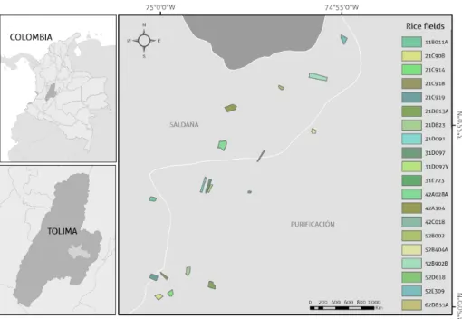
(modified after Zhao et al. (2012)). . . 23 2.1 Location map of the rice fields used for training and validationin the Saldaa region. 27 2.2 Location map of the rice fields used for testing in the Cesar region. . . 27 2.3 Overview of the methodology for processing Sentinel-2 and Landsat images. . . . 31 2.4 Example of the separable case for two classes (blue and red dots). The solid
black line represents the decision boundary. . . 33 2.5 Location of the study area with Landsat-7 true-color image (blue, green and red
bands) acquired on 7 July 2015. The black lines are regions in which there is no data. . . 39 2.6 Geometric registration results. The left and central images are the NIR
re-flectance band at 10 m measured by Landsat-8 and Sentinel-2, respectively. The right image is the cross-correlation matrix. . . 39 2.7 Boxplots of the captured NDVI reflectance distributions in each rice fields pixel
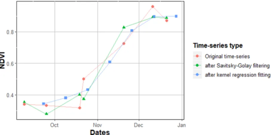
in Salda˜na at each date of interest. The lines represent the NDVI trend along the time. The colors refer to each rice growth phase. . . 40 2.8 single pixel NDVI time series comparison between initial time series (red), after
smoothing (green), and after regression (blue). . . 41 2.9 Rice growth phase that was registered in each visit date for each field. The colors
represent the growth phases. . . 42
2.10 Machine learning models results for different parameters combinations. Left: F1-score values obtained from Random Forest at a different number of trees and number of features. Right: F1-score obtained from SVM radial function that was trained with several combinations of γ and C values. The grey color represents combinations that are below 0.9. . . 43 2.11 Results of the parameter grid search for SVM polynomial basis kernel. (a) The
f1-scores for each of four parameters; (b) The f1-scores for cost and coef0 for and degree constants. . . 43 2.12 Results of the parameter grid search for XGBboost approach. (a) The f1-scores
for each of five parameters; (b) The f1-scores for cost and coef0 keeping subsam-ple, eta, and maxdepthasconstants. . . 44
2.13 f1-score per growth phase for each classification model approach. . . 45 2.14 Satellite data availability for the Cesar region. . . 45 2.15 Rice growth phase detection results for two fields in Cesar at different times. The
stacked bars compare the cumulative classification obtained per pixel. These bars are obtained at each date in which the model was computed. The ground observation data is exhibited below the bars. The lines are the technician’s registers, and the contour represents the rice field growth phase. The colors are the different classes. . . 47 2.16 Comparison between the ground observation and the estimates growth phases
per field. The points and shapes refer to the results obtained from the models at each date. . . 48 2.17 Map of rice growth estimation in Salda˜na region . . . 50 2.18 Multi-temporal characterisation for a field affected by drought. The red line
represents the date at which the technicians stopped the field monitoring. . . 51 3.1 GEE platform. The left panel contains two plots that show the time profiles for
NDVI and green, NIR, red bands. The spectral data was extracted from the Sentinel-2 and Landsat missions, these are freely available on the platform for querying. The right panel points out a true color high resolution image, which was used to draw the polygon, represented in yellow color. . . 55
3.2 Spectral response of Sentinel-2 in the visible, near infrared and short infrared range. The spectral signatures that characterise rice canopy affected by several brown spot incidence levels (blue, yellow, green and red refers to D0, D1, D2, D3, and D4, respectively) are also shown. . . 56 3.3 Location map of the rice fields located in the northern region of Tolima. . . 59 3.4 Simulated spectral reflectance response to different Brown Spot infection levels
across the Sentinel-2 spectral bands. . . 60 3.5 Results of Growth phase detection for “healthy” and “unhealthy” fields. . . 62 3.6 Sentinel-2 true color images during the reproductive and ripening periods for the
“healthy” and “unhealthy” fields. The red line is the field contour. . . 63 3.7 Spectral profiles. The red lines are the spectral information per pixel. The black
line shows the averaged spectral profiles per time. . . 64 3.8 Comparison between the simulated spectral reference and the spectral profiles for
each date and for each field (“healthy” and “unhealthy”). The colorbar indicates Euclidean distance value, which its low values are colored in dark purple, whereas high values are colored as yellow. . . 65 3.9 Comparison between the spectral reference profiles (blue and red lines) and the
rice fields averaged spectral profiles (green and orange lines) computed for both fields. . . 65 3.10 Euclidean distances result from comparing the rice fields reflectance spectral
profiles during the ripening phase. . . 66 3.11 Comparison between the reflectance spectral profiles per pixel for each field (i.e.,
“healthy” and “unhealthy” ) during the maturity stage. . . 66 3.12 Boxplots of the normalised bi-stage distributions by rice field disease status. . . 67 3.13 Number of cluster selected for the “healthy” and “unhealthy” fields. The red
points highlight which cluster were picked. . . 67 3.14 Map of the clusters calculated for the “healthy” field. The true color image is
the date in which the rice field was in the heading stage. . . 68 3.15 Averaged spectral profiles for each cluster that characterised the “Healthy” field. 68
3.16 Map of the clusters calculated for the “unhealthy” field. The true color image is the date in which the rice field was in the heading stage. . . 69 3.17 Averaged spectral profiles for each cluster that characterised the “Unhealthy”
field. . . 69 3.18 Results for three different rice fields. The map for each field is exhibited in the
left panel; The disease incidence score is pointed out above the map. In the right, the averaged spectral profile for each cluster and field. . . 70 3.19 Rice canopy spectral profiles at various nitrogen rates (Gnyp et al. (2013)). . . . 72
Abstract
New sources of information are required to support rice production decisions. To cope with this challenge, studies have found practical applications on mapping rice through the use of remote sensing techniques. This study attempts to implement a methodology aimed at mon-itoring rice phenology using optical satellite data. The relationship between rice phenology and reflectance metrics was explored at two levels: growth stages and biophysical modifications caused by diseases. Two optical moderate-resolution missions were combined to detect growth phases. Three machine learning approaches (random forest, support vector machine, and gra-dient boosting trees) were trained with multitemporal NDVI data. Analytics from validation showed that the algorithms were able to estimate rice phases with performances above 0.94 in f-1 score. Tested models yielded an overall accuracy of 71.8%, 71.2%, 60.9% and 94.7% for vegetative, reproductive, ripening and harvested categories. A second exploration was carried out by combining Sentinel-2 data and ground-based information about rice disease incidence. K-means clustering was used to map rice biophysical changes across reproductive and ripening phases. The findings ascertained the remote sensing capabilities to create new information about rice for Colombia’s conditions.
Declaration
No portion of the work referred to in this thesis has been submitted in support of an application for another degree or qualification of this or any other university or other institution of learning.
Copyright
i. The author of this thesis (including any appendices and/or schedules to this thesis) owns certain copyright or related rights in it (the Copyright) and s/he has given The University of Manchester certain rights to use such Copyright, including for administrative purposes.
ii. Copies of this thesis, either in full or in extracts and whether in hard or electronic copy, may be made only in accordance with the Copyright, Designs and Patents Act 1988 (as amended) and regulations issued under it or, where appropriate, in accordance with licensing agreements which the University has from time to time. This page must form part of any such copies made.
iii. The ownership of certain Copyright, patents, designs, trade marks and other intellectual property (the Intellectual Property) and any reproductions of copyright works in the thesis, for example graphs and tables (Reproductions), which may be described in this thesis, may not be owned by the author and may be owned by third parties. Such Intellectual Property and Reproductions cannot and must not be made available for use without the prior written permission of the owner(s) of the relevant Intellectual Property and/or Reproductions.
iv. Further information on the conditions under which disclosure, publication and commer-cialisation of this thesis, the Copyright and any Intellectual Property and/or Reproductions described in it may take place is available in the University IP Policy (see http://www.campus. manchester.ac.uk/medialibrary/policies/intellectual- property.pdf), in any relevant Thesis re-striction declarations deposited in the University Library, The University Librarys regulations (see http://www.manchester.ac.uk/library/ aboutus/regulations) and in The University’s pol-icy on presentation of Theses.
Acknowledgements
I would like to express my profound gratitude: to the RADA project, which sponsored my MPhil. To my supervisors Joseph Fennell and Sarah Bridle, who guided me with their valuable knowledge during this year. To the Colombian National Rice Growers Federation (Fedearroz) who made this study possible by providing the ground-based data. To the International Centre for Tropical Agricultura (CIAT), especially the data-driven agronomy team, which help to discover the data analysis impact on agriculture. To my beloved parents, Elcy Ariza and Jos`e Roberto Aguilar, and my brothers, Ernesto, Alex y Felipe, who are my daily motivation. To my friends that despite all, they still have support words.
Chapter 1
General Introduction
Many have contributed their knowledge and efforts for the consolidation of rice as one of the essential short-cycle crops in Colombia during the last decades. Government entities (Ministry of Agriculture and Rural Development), the National Rice Growers Federation (Fedearroz) and international research institutes (e.g., International Center for Tropical Agriculture) have played a key role in promoting rice research and improving rice production conditions. As a con-sequence, rice production in Colombia has increased from 2 tons.ha−1 in 1960 to 5.7 tons.ha−1
in 2016 (UNEP (2005)), and the rice production area has increased in 23 out of 32 departments with a total harvested area of 570,802 hectares (Fedearroz (2017)). Such expansion has turned rice into a vital crop for Colombia society (McLean et al. (2013)). Nevertheless, rice crop is ex-posed to several factors that affect its profitability (Amaya Montoya (2011)). High production cost, fluctuation on rice prices, international trades, disease outbreaks, and overproduction are some of the challenges that Colombian rice growers must face. Rice information is therefore essential in monitoring factors that may affect crop production.
Rice crop data is valuable in diverse aspects to bring farmers agronomical decisions tools (Delerce et al. (2016); Jim´enez et al. (2016)), to serve as a base in political decisions related with food security (Cihlar (2000); Dong and Xiao (2016)), and to monitor pest and disease outbreaks (Gnanamanickam et al. (2010)). Due to its importance, many efforts have been carried out to get reliable information about rice-ecosystems. One of the most common methods is through surveys. Regardless of its high accuracy, this methodology is time-consuming and hard to implement at a large scale (Mosleh et al. (2015)). After that, new sources of information are required to obtain high-frequency data at low cost. Remote sensing has gained interest due
CHAPTER 1. GENERAL INTRODUCTION 14
to its capacity to monitor crops at different scales in a cost-effective manner (Dong and Xiao (2016); Kuenzer and Knauer (2013)).
During the last decade, several studies have successfully proved the remote sensing capability on monitoring rice, creating valuable data for characterizing rice-crop conditions. Although the method has been widely implemented in countries which rice is extensively sowed (e.g., China, India, Vietnam) (Mosleh et al. (2015)), in Colombia there are few reported studies that have explored the relationship between rice and spectral satellite-derived metrics (Mart´ınez (2017)). The potential for growth phase detection can be further explored to characterise the intra-variability on rice fields. New metrics can be derived in order to monitor rice biophysical changes across phenological stages. A comprehensive assessment may link those changes to rice stresses factors such as diseases. This technology can be therefore used to identify and treat rice damages in fields (Gonz´alez-Betancourt and Mayorga-Ru´ız (2018); Wu et al. (2018)).
The purpose of this study is to establish new methods for monitoring rice growth phase and disease incidence in Colombia. The objective was focused on creating remote sensing metrics to better characterise the rice morphological and physiological changes through its growth cycle. Using ground-based information shared by Fedearroz, a methodology was developed to detect rice growth phases using optical satellite data. Using this to control for the phenological stage of the crop, a method for detecting zones affected by diseases within the rice fields was developed. The remainder of this chapter contains the background information related to remote sens-ing techniques and general aspects of rice phenology. Chapter two explains the methodology developed for rice growth phase detection by blending Landsat and Sentinel-2 images. Chapter three explores a method for detecting phenological changes caused by diseases during repro-ductive and ripening phases. Chapter 4 gives a synthesis and future works that must be done in order to validate methodologies.
CHAPTER 1. GENERAL INTRODUCTION 15
1.1
Remote sensing
Remote Sensing is a method that measures properties from an object using devices which are not in contact with (Khorram et al. (2012); Mulla (2013)). These devices can be mounted on aircrafts, earth orbiting spacecrafts, or even held by hand (ground-based). The electromagnetic energy emitted or reflected by the object is captured by the devices or sensors. Any object at a given temperature should naturally emit electromagnetic radiation. The amount of energy is proportional to the source temperature (Joshi and Kumar (2008)). The electromagnetic (EM) radiation is the energy that moves at a speed of light in a harmonic wave pattern. The EM waves comprise an electromagnetic spectrum. One property of the electromagnetic radiation is the wavelength; this is a spatial distance from one wave position to the next wave in the same point (Khorram et al. (2012)). This attribute is used to split the spectrum into seven categories: gamma rays, x-rays, ultraviolet, visible rays, infrared rays, microwaves, and radio waves (Joshi and Kumar (2008)).
One of the principal energy sources on earth is the sun. Various types of interactions can occur between EM and matter, such as absorption, reflection, scattering, emission, and transmission. Thus, a material has a characteristic absorbance and/or reflectance to the original EM radiation; this phenomenon is known as a spectral profile. The key of remote sensing is that the devices used can record the spectral profile (Khorram et al. (2012)). The sensors that detect electromagnetic radiation from natural sources are known as passive sensors. In contrast, active systems rely on illuminating the subject with a pulse or beam of radiation and measuring the backscatter. Airborne photography and optical satellites belong to the first group, while Light Detection and Ranging (LIDAR) and Radio Detection and Ranging (RADAR) are examples for the second one.
Likewise, remote sensing information can be obtained in two ways: non-imaging, and imag-ing. Sensors such as spectroradiometers which are commonly used in ground-based applications are in the first category. For the imaging methods, one example is the earth observation data that is captured by the satellites (Martinelli et al. (2015)). The digital images can be stored at different spatial, temporal, spectral, and radiometric resolutions. Spatial resolution is the image grid size. Cadence is the revisiting time on a specific geographical location. Spectral
CHAPTER 1. GENERAL INTRODUCTION 16
resolution is the sensor ability for registering wavelength intervals. Finally, radiometric resolu-tion characterises the sensor sensitivity (Khorram et al. (2012)). These parameters constrain the applicability of the product.
Currently, close to 200 Earth Observation satellites are continuously registering information (Ma et al. (2015)). This amount of data has facilitated the development of applications in many fields such as oceanography, atmospheric, weather forecasting, environmental monitoring, urban structuration, and agriculture.
CHAPTER 1. GENERAL INTRODUCTION 17
1.2
Remote sensing in agriculture
The first studies using remote sensing techniques were focused on characterizing leaf chlorophyll content (Benedict and Swidler (1961); Thomas and Gausman (1977)). This pigment absorbs energy centered in blue and red, while reflects the wavelength in green, yet, these spectral regions are not the only ones related to vegetation. Baret et al. (1987), found that the red edge spectrum provides information related to the leaf area and the percentage of ground coverage. Bannari et al. (1995), mentioned that near-infrared (NIR) is affected by leaf cellular structure. To overall the plant-spectral relationship, the reflectance in the visible spectrum is low mainly caused by photosynthetic pigments. In the red-edge region, retrieval is influenced by chlorophyll content (Ramoelo et al. (2012)). The leaf cellular structure controls the absorbance in the near infrared region. Finally, for short-wavelength infrared, the reflectance is influenced by water, proteins, and other carbon constituents content (Huang et al. (2012); Pe˜nuelas and Filella (1998)).
Since the first Earth Observation satellite mission, studies have focused on characterizing radiometric response and vegetation cover using broadband sensors. Among spectral bands, red and NIR especially showed high sensitivity to vegetation conditions. The red band is absorbed by chlorophyll that is essential for the plant photosynthetic process, while NIR is reflected by leaf cellular structures. Thus, the combination of both bands allows identifying vegetation covers from others (e.g., soil, and water) and quantify the vigor of the plant (Bannari et al. (1995)).
The quantification metrics derived from spectral band combinations are known as vegeta-tion indices. The first indices were computed as ratios of the green and NIR bands. Although these ratios are used to measure relative greenness, these indices may be affected by atmo-spheric effects, vegetative density, and study location (Bannari et al. (1995); Tucker (1979)). Rouse et al. (1973), found a way to reduce the negative aspect of existing vegetation indices by calculating the normalised difference between red and NIR bands. Thus, the normalised dif-ference vegetation Index (NDVI) gained notorious importance for plant biophysical properties monitoring. However, the NDVI is sensitive to soil background, atmospheric conditions, and heterogeneous canopies (Rondeaux et al. (1996); Xue and Su (2017)). To adequately assess the plant response using band combinations, many studies have developed different vegetation
CHAPTER 1. GENERAL INTRODUCTION 18
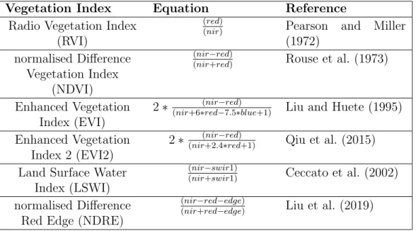
indices to tackle specific problems (table 1.1).
Table 1.1: List of standard vegetation indices, and their mathematical equation.
Vegetation Index Equation Reference
Radio Vegetation Index (RVI)
(red)
(nir) Pearson and Miller
(1972) normalised Difference
Vegetation Index (NDVI)
(nir−red)
(nir+red) Rouse et al. (1973)
Enhanced Vegetation Index (EVI)
2∗ (nir+6∗(rednir−−7red.5∗)blue+1) Liu and Huete (1995) Enhanced Vegetation
Index 2 (EVI2)
2∗(nir(+2nir.−4∗redred)+1) Qiu et al. (2015) Land Surface Water
Index (LSWI)
(nir−swir1)
(nir+swir1) Ceccato et al. (2002)
normalised Difference Red Edge (NDRE)
(nir−red−edge)
CHAPTER 1. GENERAL INTRODUCTION 19
1.3
Rice phenological detection
Rice phenology can be divided into three main phenological phases: vegetative (germination to panicle initiation), reproductive (panicle initiation to flowering), and maturity or ripening (grain filling to maturity)(Moldenhauer and Slaton (2001)). Changes in the plant morphology characterise each agronomic stage. The vegetative phase initiates with the plant emergence; during this phase, the main characteristics are the gradual increase of plant height, leaf area, and an active tillering. The phase transition takes place when the tiller number per plant reaches a maximum. The reproductive stage follows maximum tillering. During this phase, the panicle primordia stage starts its initiation. The panicle needs approximately 25 days to achieve the heading stage, which refers to when 50% of the panicles have flowered. After 100% of flowering, the ripening stage takes place. The maturity stage is characterised by leaf senescence and grain filling (Yoshida (1981)). The rice cycle takes from 3 to 5 months; the difference is subject to the conditions in which the crop is developed (Kuenzer and Knauer (2013)).
Figure 1.1: Rice plant cycle with phase and froth stages. the curve represents the temporal profile for NDVI (modified after Kuenzer and Knauer (2013); Mosleh et al. (2015)).
As the rice plant change its growth phenology, the reflectance is affected at different spectral wavelength. Studies have adequately described the rice cycle as a function of vegetation indices. Several indices have shown a strong correlation with rice growth. For example, NDVI is affected by the low percentage of vegetation cover at the early vegetative phase, due to that its values are close to zero (figure 1.1). While the plant is growing, the chlorophyll quantity increases,
CHAPTER 1. GENERAL INTRODUCTION 20
which exerts considerable influence in the absorbance of light in the red domain. Although the absorbance in the blue region also increments due to chlorophyll content, this domain is also influenced by carotenoids absorption (Pe˜nuelas and Filella (1998)). In NIR region, the reflectance is increased by foliar and tillering development. The NDVI characterises this process as a gradual increment in its values. Finally, NDVI starts to decrease due to biomass reduction (decay and loss of leaves), greenness diminishing (chlorophyll content), and yellowness increase (rice grains filling)(Kuenzer and Knauer (2013); Mosleh et al. (2015)).
The growth stage can, therefore, be predicted by the NDVI trajectory in time. Several stud-ies have shown the feasibility in detecting rice phenological changes using time-serstud-ies NDVI reg-istered by satellite missions. Frequently studies referred to MODIS vegetation indices products that can produce NDVI and EVI on 16 days intervals at multiple spectral resolutions (NASA (2018)). Thus, Sakamoto et al. (2005) and Shihua et al. (2014) used EVI multi-temporal profiles to characterise the rice cycle. Three phenological dates (planting, heading, and harvest) were calculated based on the inflection points that were found in the time-series. Although MODIS products have a high temporal resolution (the products are staked from a daily measurement), their spatial resolution is low (>250 m), which hampers a precise identification (Onojeghuo et al. (2018)).
Other studies have focused their analysis on satellites with higher spatial resolution than MODIS, such as Landsat or Sentinel-2. Nevertheless, their low temporal resolution compromises data availability. Recent methodologies merge multiple mission to overcome this inconvenience. For instance, Wang et al. (2015) created smoothed vegetation indices time-series by combining two optical satellites, Landsat-8, and HJ-1 CCD. They found reliable performances when both satellites were combined, instead of using only one. They assigned the rice phenological shift for those days when the vegetation index time-series reached a maximum. Wu et al. (2018) used radar and optical data to detect rice in early middle, and late phases for areas located in China. Thus, they summarized Sentinel-1s VH backscattering images taken during the rice plantation period in three layers minimum, difference, and maximum. The imagery stack was compared with the minimum and maximum coefficients, which defined the rice growth stages. Finally, they calculated the Landsat-8’s NDVI values for which areas filtered from the Sentinel-1. The NDVI was classified using the k-means approach to differentiate each rice stage. Although the
CHAPTER 1. GENERAL INTRODUCTION 21
study reported a high level of overall accuracy (98.1 %) in their methodology, they worked under local rice system conditions, for example, assuming a general crop calendar and considering only irrigation rice
CHAPTER 1. GENERAL INTRODUCTION 22
1.4
Crop diseases detection
Plant pathogens are significant causes of yield loss (Huang et al. (2012)). The primary or-ganisms that cause damage to rice plants are bacteria, viruses, fungi, and nematodes (Ahn and Jennings (1982)). Hence, many efforts have risen in order to understand the symptoms caused by the pathogens, as well as to better characterise the specific environmental condi-tions that facilitate their outbreaks. For example, The Centre for Tropical Agriculture (CIAT) and Fedearroz have identified five significant pathogens for Colombia (Correa-Victoria and Zei-gler (1993); Fedearroz (2014)). These are Pyricularia Orizae, Helminthosporium, Rhizoctonia Solani, Rhynchosporium, Gaemannomyces.
Rice blast disease is caused by the fungal pathogen Pyricularia Orizae (teleomorph Mag-naporthe Orizae); this is of considerable importance to rice producers (Dean et al. (2012)). The fungus affects all foliar tissues, and the major diagnostic symptoms are lesions on leaves, nodes, and different parts of the panicle (Ou (1985)). Although the disease is reported world-wide, symptoms depend on the climatic conditions, especially relative humidity (Ou (1985)). For example, in Colombia, the rice blast is mainly located in the eastern part of the country due to a suitable temperature and humidity conditions (Correa-Victoria and Zeigler (1993); Fedearroz (2014)). The establishes during early plant stages, tillering and neck emerge stages are susceptible to this pathogen (Venkatarao and Muralidharan (1982)) and is immediately controlled by farmers when symptoms present.
Different factors affect the incidence of Brown Spot disease (Helminthosporium Orizae), but, environments with a scarce water supply and lacking in soil nutrient minerals, or with accumulated toxic substances, facilitated the diseases development (Ou (1985); Barnwal et al. (2013)). Indeed, Ou (1985) reported that Brown Spot disease is caused by a deficiency of one or more nutrient elements (nitrogen, silica, potassium manganese, and magnesium), and in practice, disease and deficiency symptoms are often inseparable. Thereby, the Brown Spot is sometimes used as a reference to mineral deficiencies (Ahn and Jennings (1982); Daytnoff et al. (1991); Barnwal et al. (2013)). Plant age is also relevant for disease growing. Although Brown Spot can attack at early plant stages, its damage is commonly noted in dough and maturity stages (Singh (2016)).
CHAPTER 1. GENERAL INTRODUCTION 23
content. Consequently, the electromagnetic spectrum absorption at different wavelengths varies depending on the level of disease. For instance, one symptom of Magnaporthe Orizae is leaf cell necrosis, which causes pigments degradation; these changes can be therefore spotted by the visible spectral region (Zhou et al. (2019)). Kobayashi et al. (2001) reported that blue and red regions reflectance increases at dough stage, because of the carotenoids and chlorophyll content decrement. Pathogens such as Rhizoctonia and Helminthosporium also have been detected using the visible and NIR regions (Qin and Zhang (2005)). For instance, Liu et al. (2008) and Zhao et al. (2012) characterised rice infected with Helminthosporium Oryzae using hyperspectral ground-measurements taken at a laboratory and field-canopy level, respectively. They found differences in the near-infrared spectrum, specifically at the ranges of 740 nm to 790 nm and 1550 nm to 1750 nm, comparing healthy and diseased rice (figure 1.2). Zheng et al. (2018) proposed a new index vegetation index, red-edge disease stress index (REDSI), for detecting yellow wheat rust at canopy and plant level using Sentinel-2. Zhihao Qin et al. (2003) identified rice incidence on Rhizoctonia Solani combining four broad bands that were captured by airborne. Thus, they pointed out that the disease incidence correlated to indexes calculated from blue, red, red-edge, and NIR band values.
Figure 1.2: Rice-canopy spectral profiles for four severity levels of Helminthosporium Oryzae (modified after Zhao et al. (2012)).
The practical implementation of remote sensing has been hampered by differentiating the disease from other stress factors (e.g., lack of nutrients or drought) which can trigger similar changes in reflectance (Huang et al. (2012); Liu et al. (2019)). Recent studies have blended
CHAPTER 1. GENERAL INTRODUCTION 24
hyperspectral and multi-temporal satellite data. Shi et al. (2018) mapped rice damage from diseases using two different acquisition dates from the high spatial resolution PlanetScope. Huang et al. (2012) firstly characterised yellow rust on wheat using hyperspectral ground-based measurements that then was used as a reference for satellite implementation. Although PlanetScope offers useful information at high spectral and temporal resolutions, their images ac-quisition prices constrain regional application. These studies show the potential use of spectral reflectance measurements in quantifying the incidence or severity of rice diseases.
Chapter 2
Rice Growth Phases Detection
In this section, a novel approach for identifying rice growth phases using optical satellite im-ages and supervised classification approaches is presented. Sentinel-2 and Landsat data were downloaded and processed for two localities in Colombia. Three state-of-the-art machine learn-ing supervised classification algorithms (random forest, support vector machine, and gradient boosting trees) were trained, validated, and tested using ground-based data shared by The Colombian National Rice Growers Federation (Fedearroz). The analysis showed: 1) clear re-lationship in various rice growth phases with multi-temporal NDVI data; 2) feasible to obtain a considerable number of optical satellite data by blending Landsat and Sentinel-2 missions; 3) training supervised classification approaches allowed applying the methodology in another locality.
CHAPTER 2. RICE GROWTH PHASES DETECTION 26
2.1
Materials and methods
2.1.1
Study areas
Two sites in Colombia were chosen to train and test the spatial phenological detection approach using optical images. Salda˜na and Purificaci´on are two Tolima municipalities that cover nearly 21,400 hectares from 4°N and 75°6.01'W to 3°48.6'N and 74°54.475'W. The zones are in the central part of Colombia. The municipalities temperature ranges from 27°C to 28.5°C over the year. Precipitation has a bimodal distribution spanning from March to May and from September to November. The climatic conditions are suitable for rice production, which has influenced the local economic activity (Delerce et al. (2016)). Thus, the agricultural sector is responsible for almost 77% of the municipalities’ Gross Value Added (Fedearroz (2010)). The rice annual planting area is nearly 15,390 hectares in both localities. Hereafter the name Salda˜na is used to refer to both municipalities.
The second site is in the Cesar department. The Cesars climate is classified as tropical wet and dry. The wet season begins in March, and dry season starts in December, with an average annual temperature that ranges from 27°C to 34°C. This region has specific crop management differences compared with Salda˜na. The most notable is the farming system. While lowland irrigated rice is the only system implemented in Salda˜na, in Cesar the 5% of the system is rainfed rice (DANE (2017)), which means that irrigation only depends on the rainfall duration.
2.1.2
Ground data
The Colombian National Rice Growers Federation (Fedearroz) collected the ground data as part of a separate initiative. Twenty rice fields plantations were monitored in the second semester of 2015 (figure 2.1). Rice fields were visited on five dates from November 2015 to January 2016. Rice growth stages, field geospatial location, plant height, soil water content, emergence date, field extension, and an overall appreciation over rice cycle conditions were variables included in the survey. A second campaign was undertaken in 2018 in the Cesar department. Nineteen rice fields were surveyed (figure 2.2). The new data allowed testing models on a new geographic area with slightly different climatic conditions. In addition to the parameters measured above, any external incidence, such as drought or agronomic practices, was also included.
CHAPTER 2. RICE GROWTH PHASES DETECTION 27
Figure 2.1: Location map of the rice fields used for training and validationin the Saldaa region.
CHAPTER 2. RICE GROWTH PHASES DETECTION 28
2.1.3
Satellite data
Sentinel-2
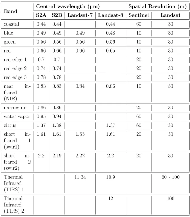
The Sentinel-2 mission is part of the Global Measurement for Earth and Security (GMES) pro-gram, which is responsible for delivering data products for environmental and security services (Drusch et al. (2012)). Sentinel-2 reflectance measurements provide essential data for stud-ies of land management, agriculture, and disaster monitoring (Aschbacher and Milagro-P´erez (2012)). Sentinel-2 has two identical satellites with revisit cycle of 10 days. Thus, the mission captures information globally every five days. Each satellite has a Multispectral Instrument (MSI), which is used to monitor the earth surface in 13 spectral bands (table 2.1). The instru-ment has a spectral range from the visible to the short wave infrared (Drusch et al. (2012)). The spatial resolution varies regarding the wavelength, thus visible and NIR are available at 10 m, while red-edge and SWIR are recorded at 20 m. All data were downloaded directly from the Sentinels Scientific Data Hub (https://scihub.copernicus.eu/ ).
Landsat-7 and Landsat-8
The first Landsat mission was launched in 1972. Since then, six satellites were put into orbit to monitor the global earth surface. This program has been led by the National Aeronautics and Space Administration (NASA) and the United States Geological Survey (USGS). The Enhanced Thematic Mapper Plus (Landsat-7 ETM+) and the Operation Land Imager (Landsat-8 OLI) are two satellites which are still capturing data every 16 days. Both can scan surface reflectance and land surface temperature as a result of measuring the visible, near infrared, and short wave infrared portions of the spectrum (Claverie et al. (2018))(table 2.1). USGS processes Landsat-8 and Landsat-7 surface reflectance products that are then distributed in the EarthExplorer repository (https://earthexplorer.usgs.gov). The available data has the highest-level quality and is achieved through two processing softwares, Landsat Ecosystem Disturbance Adaptive Processing System (LEDAPS) and the Landsat Surface Reflectance Code (LaSRC), designed for Landsat-7 and Landsat-8 respectively. Although both products are processed using different data sources, their inputs are water vapor, ozone, geopotential height, aerosol optical thickness, and digital elevation (USGS (2018a,b)). Unfortunately, the Landsat-7 scan line corrector (SLC) failed in 2003. The SLC controls the forward motion of the satellite. Therefore, close to 22%
CHAPTER 2. RICE GROWTH PHASES DETECTION 29
of the pixels of the data are missing since then (Chen et al. (2011)).
Table 2.1: Corresponding central wavelength and spatial resolution available at each band for each instrument.
Band
Central wavelength (µm) Spatial Resolution (m) S2A S2B Landsat-7 Landsat-8 Sentinel Landsat
coastal 0.44 0.44 0.44 60 30 blue 0.49 0.49 0.49 0.48 10 30 green 0.56 0.56 0.56 0.56 10 30 red 0.66 0.66 0.66 0.65 10 30 red edge 1 0.7 0.7 20 30 red edge 2 0.74 0.74 20 30 red edge 3 0.78 0.78 20 30 near in-frared (NIR) 0.83 0.83 0.84 0.86 10 30 narrow nir 0.86 0.86 20 30 water vapor 0.95 0.94 60 30 cirrus 1.37 1.38 1.37 60 30 short in-frared 1 (swir1) 1.61 1.61 1.65 1.61 20 30 short in-frared 2 (swir2) 2.2 2.19 2.22 2.2 20 30 Thermal Infrared (TIRS) 1 11.34 10.9 60 - 100 Thermal Infrared (TIRS) 2 12 100
2.1.4
Satellite images processing
Surface reflectance
Atmospheric variability (e.g. from clouds, water vapor, dust, etc.) must be corrected in order to recover the Bottom of Atmosphere Reflectance (Chen and Cheng (2012); Tian et al. (2018)). In Sentinel-2, such process is carried through the state version of sen2cor. The module uses two
CHAPTER 2. RICE GROWTH PHASES DETECTION 30
external sources, radiative transfer tables and a digital elevation model (DEM). The tables con-tain absorbance as a function of the frequency, pressure, temperature, and water vapor (Buehler et al. (2011)). The atmospherically corrected product also contains a Scene Classification Layer, providing a broad classification of the ground cover at a 400m2 resolution.
Sentinel-2 and Landsat data work with different spatial resolution levels. An image resam-pling was applied to compare the reflectance of data sources. Considering that 10 meters are the highest spatial resolution available for the data, this was selected as a reference for all products. There are several techniques developed for image resampling purposes. This study used two: bilinear spatial interpolation and nearest neighborhood. The first algorithm takes the nearest cells values and applies them an average. Hence, the new value will be the mean of their neighborhoods. This model was applied on images with continuous numeric data, and for categorical layers (e.g., the scene classification layer) were processed using the nearest neigh-borhood method. This model, as its name refers, assigns the pixel of interest value equal to its most adjacent pixels.
Landsat geometric registration
Studies have revealed the existence of misregistration between Landsat and Sentinel-2 products. Some have reported a shift of up to 1.6 pixels at 30 meters resolution. Thus it is advisable to apply a co-registration method to the images (Skakun et al. (2017)). For this reason, many methodologies have been developed for geographic correction. This study uses phase correlation, which was reported in Skakun et al. (2017). The phase correlation algorithm is based on the cross-correlation algorithm that transforms both images into a Fourier space. The peak of the cross-correlation represents the shift that must be applied to the register image (Guizar-Sicairos et al. (2008)).
One Sentinel-2 image and one Landsat-8 were chosen considering two conditions: 1) the acquisition dates are the same for both images, and 2) the cloud cover over the region is close to zero. Both images were subset for the corresponding area of interest (i.e., Salda˜na extension). The final registered imagery had a 10 m spatial resolution.
CHAPTER 2. RICE GROWTH PHASES DETECTION 31
Figure 2.3: Overview of the methodology for processing Sentinel-2 and Landsat images.
2.1.5
Vegetation index time series processing
The multitemporal stacked layers were used as input for the vegetation time series creation. The red and NIR bands were extracted from each adquisition image; these bands were used to compute the NDVI layer. Each pixel had information about the vegetation index throughout time. However, values from a multi-temporal sequence can be affected by the presence of noise (e.g., atmospheric, surface reflectance methods, shadows). Therefore, a filtering technique is necessary for handling these errors. The Savitzky-Golay algorithm was chosen, which uses a moving window to smooth values that span into it (Savitzky and Golay (1964); Cao et al. (2018)). The smooth approach has two parameters: the window size and the polynomial fitting degree. To summarize the NDVI time series, five features were calculated.
The rice growth phenological phase detection problem has been addressed through charac-terising in which dates the NDVI time profile has inflection points, these changes may describe the shift into a new growth phase (Shihua et al. (2014)). Thus, the inflection points are obtained from derivatives methods. In this study, two derivatives values were computed at beginning and ending of the smoothed time series. Additionally, five features were obtained aimed at summarizing the NDVI time series.
CHAPTER 2. RICE GROWTH PHASES DETECTION 32
The kernel regression method was applied in order to estimate new values across the time series. The simplest kernel weights average estimation is the Nadaraya Watson form (Hastie et al. (2009)): fb(x0 ) = Pn i=1Kλ(xi, x0)y0 Pn i=1Kλ(xi, x0) (2.1) Where, Kλ is a gaussian kernel function for λ which controls the variance of the gaussian
density. This regression was performed for every pixel in the multi-temporal stack. The result-ing NDVI time series is composed of seven points that are separated by 16 days. Finally, 14 features were created for classification (table 2.2)
Table 2.2: List of features used in the models.
Feature Name Meaning
NDVI 1 NDVI value for 96 days before the date of interest.
NDVI 2 NDVI value for 80 days before the date of interest.
NDVI 3 NDVI value for 64 days before the date of interest.
NDVI 4 NDVI value for 48 days before the date of interest.
NDVI 5 NDVI value for 32 days before the date of interest.
NDVI 6 NDVI value for 16 days before the date of interest.
NDVI 7 NDVI value for 0 days before the date of interest.
NDVI sd ts Standard Deviation of the NDVI time series.
NDVI max ts Minimum NDVI value.
NDVI min ts Maximum NDVI value.
maximum NDVI day day in which the NDVI time series reached a maxi-mum.
minimum NDVI day day in which the NDVI time series reached a mini-mum.
first derivative tsending value on the date of interest for a first derivative of the NDVI time series.
first derivative tsstarting value on 80 days prior the date of interest for a first derivative of the NDVI time series.
2.1.6
Supervised classification algorithms
Herein, three classification approaches were used and compared in this study: support vec-tor machines, random forest, and gradient boosting machine. The implementation of each algorithm was done through packages that were developed for the software R. Support vector machine, and random forest modes have been widely used in remote sensing studies (Mountrakis et al. (2011); Belgiu and Drgu (2016)). Recently, gradient boosting machine has gained noto-rious popularity because of its superior performances compared to more traditional machine
CHAPTER 2. RICE GROWTH PHASES DETECTION 33
learning techniques (Georganos et al. (2018)).
Support Vector Machines
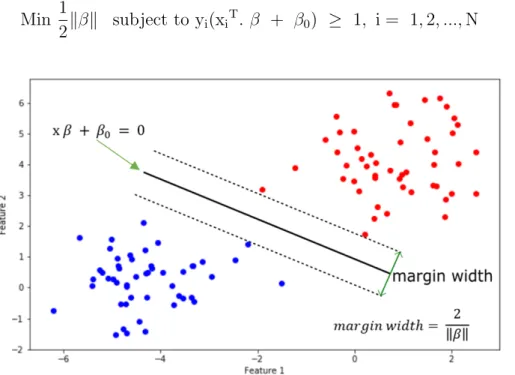
The support vector machines (SVM) is based on the linear model classification, which uses a hyperplane for class separation. A linear function is suitable for the cases where the data is linearly separable. The optimal hyperplane is one that maximizes the margin width between the nearest classes (figure 2.4). This margin depends on one vector (β) which is perpendicular to the linear function. Therefore, the unknown point classification depends on its location, considering the hyperplane. Thus, to maximize the margin, the algorithm finds the minimum distance from the origin vector (β)
Min 1
2kβk subject to yi(xi
T. β + β
0) ≥ 1, i = 1,2, ...,N (2.2)
Figure 2.4: Example of the separable case for two classes (blue and red dots). The solid black line represents the decision boundary.
Although the hyperplane was conceived to separate the classes as best as possible, there are cases where categories are overlapping in the feature spaces. Thus, this scenario is tackled by allowing errors when data are separated (Cortes and Vapnik (1995)). The errors can be expressed as εi which are greater or equal to 0. The total of errors is also constrained by a
constant (C), aimed to regularise the function PN
i εi ≤ C. Thus, large C values allow the εi
CHAPTER 2. RICE GROWTH PHASES DETECTION 34
model will be restricted (Hastie et al. (2009)). Adding cost values to all points that violated the constraints, the optimization problem is defined as:
Min 1 2β 2 + C N X i εi subject to εi ≥ 0, yi(xiT. β + β0) ≥ 1 − εi, i= 1,2, ..., N(2.3)
Linear separation models work accurately under scenarios where a linear function can sep-arate the data, but for data with a more complex distribution, it is necessary to add new non-linear features. However, the transformation and selection of new features require con-siderable computational resources that make it challenging to find new solutions (Muller and Guido (2017)). Cortes and Vapnik (1995), found a way to deal with this problem, they demon-strated that it is not necessary to transform the new feature. It is only required to obtain the inner products (e.g., dot product) from a small amount of training data. After that, a non-linear transformation is applied to the vectors. The training points are known as support vectors. The inner product in the new space is found through a kernel function. Two of the more commonly used functions, in support vector machines, are polynomial kernel and radial basis function.
Polynomial kernel basis : K (xi,x) =
xiTx + coef
d
(2.4) Radial basis function : K (xi,x) = exp−γ ||xi−x ||2 (2.5)
SVM is sensitive to feature magnitudes, so all features must have the same scale. Although NDVI data ranges from 0 to 1, the other features values oscillate on another scale. For this reason, the min-max normalisation method was used to transform all data on the same scale [0,1].
Random Forest
Random Forest is an ensemble model of a finite number of decision trees. The tree models recursively split the data into subsets through a serial of rules. However, when a tree has many splits, it can overfit the data. On the one hand, this model has a straightforward interpretation of the results. On the other hand, the model is unstable, and the final pruning will depend on
CHAPTER 2. RICE GROWTH PHASES DETECTION 35
the primary partition. Breiman (2001) showed significant improvements in reducing overfitting and variance scenario on tree based approaches, through training many trees with random data; thus, each tree casts a class, and the final decision depends on the number of votes.
The new training sets are drawn from randomising the original data with replacements (the same point can be picked more than one time). This method is known as bootstrap (Breiman (2001); Muller and Guido (2017)). Using bootstrap, we can obtain multiple datasets that have the same length than the original dataset. The bootstrap aggregation or bagging is the results of averaging the models’ predictions fitted with the bootstrap samples. This technique reduces high-variances and low-biased obtained from approaches such as trees (Hastie et al. (2009)).
Additionally, to ensure that each tree grows independently, a random subset of the features is used in each node. Consequently, the trees can predict based on different features combinations. Therefore, the grown trees are not pruned. Two parameters are needed to construct a random forest model: the number of trees and the maximum number of features used at each node.
Gradient Boosting Trees
Gradient boosting is another ensemble model based on trees approaches. However, instead of using bootstrap as a sampling method, it uses the boosting method. Contrasting with random forest, with which predictions are derived from multiple bootstrap samples, gradient boosting machine is a way of combining the performance of many weak classifiers to improve the general performance additively (Friedman et al. (2000); Muller and Guido (2017)). Thus, for the tree based approach, the trees grow in an adaptative way to reduce bias (Hastie et al. (2009)).
In general, the learning model aimed to train a function F(x) using a training sample ({xi, yi}N1 ) that minimises the expected value (E) of some specified loss function Friedman
(2001) is:
ϕ(F(x)) = arg min
F E
x[EyL(y, F(x)))|x] (2.6)
In order to find a solution for ϕ(F(x)), Friedman (2001) proposed an alternative where the model is trained in an additive way. Thus, the solution is obtained from the previous approximation,t−1. This strategy is known as stagewise-greedy or gradient boosting procedure.
CHAPTER 2. RICE GROWTH PHASES DETECTION 36 F(x)t =F(x)t−1 +αh(x)t (2.7) ϕ(F(x))= arg min F E x[EyL(y, F(x)t −1 +αh(x)t)|x], (2.8) where α is a step size and the function h(x) is a base predictor (or also known as a weak learner) that belongs to the family functions F, which usually are classification trees. One inconvenience in this model is the tendency to overfit the data. This problem has been tackled with multiple algorithms. Among the gradient boosting machine implementations, XGBoost has proved to have good performances in many studies. The method implements stronger regularization parameters that constrain the model (Georganos et al. (2018)). For the purpose of the study, five parameters were modified. The learning rate (eta), col sample (percentage of columns using in each tree), gamma (the loss reduction), max depth (maximum depth of the tree), and sub sample (ratio of the training set) (Chen and Guestrin (2016)).
2.1.7
Evaluation metrics and scoring
The performance of each supervised classification approaches was assessed through metrics that compare predictions to real values. The confusion matrix method is commonly used for binary classification (table 2.3). Although the confusion matrix is an efficient tool to visualise performances, the matrix by itself lacks a metric to evaluate the classification. However, some techniques allow summarising the confusion matrix. Precision, recall, and f1-score are evalua-tion metrics that are commonly used not only for binary classificaevalua-tion but also for multi-class problems (Sokolova and Lapalme (2009)).
Table 2.3: Confusion matrix for binary classification.
Real Positive Real Negative Predicted Positive true positive (TP) false positive (FP)
Predicted Negative false negative (FN) true negative (TN)
Precision is the proportion of samples classified as positive by the model, which are truly positive. Recall measures the ratio of the amount of correct positive classifications to all possible positive values in the data (Lantz (2013); Muller and Guido (2017)). F1-score is the harmonic mean of precision and recall. Micro averaging, macro averaging, and per-instance averaging
CHAPTER 2. RICE GROWTH PHASES DETECTION 37
are variations of the three mentioned metrics that are applied to multi-class problems (Lipton et al. (2014)). Micro is the sum of all true positive (TP), false positive (FP), true negative (TN), and false-negative (FN) quantities for all classes. Whereas, macro averaging calculates the parameters per class, and then averages the results. Finally, per-instance averaging assigns weights to each class. Macro averaging is used when the methodology requires to treat all categories as equal, yet in cases when bigger classes must be favored, the micro averaging is computed (Sokolova and Lapalme (2009)). In this study, the macro averaging metric is applied to gauge the model performances.
Precision macro = C X i=1 T Pi T Pi+T Pi (2.9) Recall macro = C X i=1 T Pi T Pi+F Ni (2.10)
f1 Score macro = 2 Precision∗Recall
(Precision+Recall) ∗ C (2.11)
Training machine learning approaches involves tuning several parameters that may impact the final robustness of the model (Verrelst et al. (2012)). A cross-validation method was com-puted to select the best tuning parameters values. Once the model classified the validation data, the f-1 score macro metric was computed to measure the model performance. Finally, the parameters configuration for which f1-score was the highest was selected. Each supervised classification approach varies in the number of parameters to optimize. For instance, ran-dom forest only depends on the trees numbers and features used as input at each node. On the other hand, SVM polynomial kernel has four parameters to modify: regularization (cost), polynomial-degree, γ, and initial coefficient (coef0).
CHAPTER 2. RICE GROWTH PHASES DETECTION 38
2.2
Results
2.2.1
Optical images pre-processing
Twelve Landsat and four Sentinel-2 images were downloaded (table 2.4). The MSI images were atmospherically corrected using the Sen2Cor module, while for Landsat, the surface reflectance product was directly obtained from USGS. All images were projected to Universal Trans Merca-tor projection (UTM Zone 18N) and then clipped using a mask that encompassed the Salda˜na region. A noise percentage index was calculated using the scene layer classification to indicate the percentage of clouds and shadows over the interested region. Although for Landsat-7 im-ages, this index shows relatively low values, it must be considered the error caused by the SLC control, which adds another 22% of unusable pixels in the image (figure 2.5)
Table 2.4: List of Sentinel-2 and Landsat images used in Salda˜na Mission Date Cloud Percentage
Landsat-7 07-07-2015 21.68 Landsat-7 23-07-2015 6.5 Landsat-8 31-07-2015 12.27 Landsat-8 01-09-2015 5.75 Landsat-7 09-09-2015 10.12 Landsat-7 25-09-2015 3.59 Landsat-8 19-10-2015 4.18 Sentinel-2 22-10-2015 12.03 Landsat-8 22-11-2015 33.24 Landsat-8 06-12-2015 50.77 Sentinel-2 11-12-2015 3.08 Sentinel-2 21-12-2015 2.21 Landsat-7 30-12-2015 27.24 Sentinel-2 10-01-2016 15.27 Landsat-7 15-01-2016 17.29 Landsat-8 23-01-2016 31.97
The geometric registration was achieved using one Landsat-8 image that was taken on 22 of December, and one Sentinel-2 product captured on 21 of December. The NIR reflectance band from both images was used because this band is less affected by atmospheric effects (Skakun et al. (2017)). The OLI band image has a spatial resolution of 30-meter; thus, a bilinear interpolation was applied to obtain a 10-meter. Once both layers shared similar spatial resolution and extension. To calculate the shift, the phase correlation method was used and implemented with the Scikit-learn python package (figure 2.6). As a result, the shift in longitude
CHAPTER 2. RICE GROWTH PHASES DETECTION 39
Figure 2.5: Location of the study area with Landsat-7 true-color image (blue, green and red bands) acquired on 7 July 2015. The black lines are regions in which there is no data.
and latitude between both images were 10 and 40 meters, respectively. Due to ETM+ and OLI products share the same registration grid, the same shift is thus applied for both. Finally, the NDVI layer was calculated for each image.
Figure 2.6: Geometric registration results. The left and central images are the NIR reflectance band at 10 m measured by Landsat-8 and Sentinel-2, respectively. The right image is the cross-correlation matrix.
2.2.2
NDVI time profiles
The five ground survey days were chosen as a reference to extract the NDVI time profile of each field. Each rice field was drawn as a polygon and used to extract the NDVI information per date. the NDVI time profiles were extracted from 130 days prior to the date in which the survey
CHAPTER 2. RICE GROWTH PHASES DETECTION 40
to the survey date. The NDVI profiles was thereafter assigned to each rice field and labeled with the growth-phase stage that was registered by the technician (figure 2.7). Although the rice fields were monitored using growth-stages notation, this phenological characterisation may not be adequately identified by the satellite approach used in this study (Wang et al. (2014)). Therefore, the growth stages were grouped into three major phenological phases: vegetative, reproductive, and ripening.
Figure 2.7: Boxplots of the captured NDVI reflectance distributions in each rice fields pixel in Salda˜na at each date of interest. The lines represent the NDVI trend along the time. The colors refer to each rice growth phase.
Two additional classes, soil and other, were added to the analysis. The first characterises the rice fields cover during two scenarios: 1) one month after being harvested, and 2) one month before the sowing date. The second category aimed at representing pixels that do not have enough information to construct a proper NDVI time series and to encompass values with an anomalous tendency. Two additional steps were applied to the NDVI time profile: smoothing and fitting.
2.2.3
Training features
The Savitzky Golay smoothing method (Savitzky and Golay (1964)) was used to smooth the NDVI time profiles (figure 2.8). The method depends on two parameters: window size and
CHAPTER 2. RICE GROWTH PHASES DETECTION 41
polynomials degree. Both parameters were modified according to the number of time points available per pixel. The kernel regression was computed on the NDVI data available in each ranged time. The cross-correlation method was applied to find the bandwidth parameter; the regression was calculated with 70% of the data; the remaining points were used to validate each estimation. Seven different values of the NDVI that describe the pixels multi-temporal reflectance were obtained. Figure 2.8 shows the three different NDVI profiles obtained from the smoothing and fitting steps applied to one pixel data.
Figure 2.8: single pixel NDVI time series comparison between initial time series (red), after smoothing (green), and after regression (blue).
2.2.4
Training and validation sets
Although all rice fields were monitored during one crop season, not all of them were sowed at the same time. Thus, some of them started to be monitored at the end of their crop cycle (e.g., rice field 52B002, figure 2.9). This condition affected the number of observations per growth phase. Other limitations were: the number of cloud-free images during the evaluation time, and the rice fields extension.
The data were randomly divided into six subsets/folds. The number of groups was chosen considering the total amount of rice fields per stage. Data were split based on the number of rice fields per growth phase, instead of the number of pixels per class. Thus, the pixels within each rice field may share similar NDVI features. The information per fold at each growth-phase was split into two sets: 70% for training, and 30% for validation. Table 2.5 summarizes the number of pixels from each group in each label as well as the pixel amount destinated for validation and training.
CHAPTER 2. RICE GROWTH PHASES DETECTION 42
Figure 2.9: Rice growth phase that was registered in each visit date for each field. The colors represent the growth phases.
Table 2.5: Model inputs per fold and growth phase.
Set Folds
Growth Phase
vegetative reproductive ripening harvested soil other
Training 1 3642 3787 2339 2155 2425 2170 2 3310 3760 2800 2194 2827 2170 3 3175 3457 2954 2530 2505 2170 4 3399 3937 2655 2294 2521 2170 5 3730 3686 2617 2230 2060 2170 6 3656 4038 2684 2155 2661 2170 Validation 1 753 1419 1278 814 877 930 2 688 1446 817 775 475 930 3 870 1749 663 439 797 930 4 646 1269 962 675 781 930 5 665 1520 1000 739 1242 930 6 739 1168 933 814 641 930
2.2.5
Parameters grid search
The random forest model was computed on 108 different parameters combinations when the number of features sampled at each split, was four (figure 2.10). The increment in the number of trees had no significant relevance in the f1-score. From the SVM radial basis kernel, the best results were obtained using a γ value equal to 0.0001 and a regularization parameter equal to 3600 (figure 2.10).
SVM polynomial basis kernel and XGBoost have more than two parameters to optimise; hence, to gauge the influence that each parameter exerts on the model, the f1-scores results were grouped for each parameter, and then were averaged.
CHAPTER 2. RICE GROWTH PHASES DETECTION 43
Figure 2.10: Machine learning models results for different parameters combinations. Left: F1-score values obtained from Random Forest at a different number of trees and number of features. Right: F1-score obtained from SVM radial function that was trained with several combinations of γ and C values. The grey color represents combinations that are below 0.9.
Figure 2.11: Results of the parameter grid search for SVM polynomial basis kernel. (a) The f1-scores for each of four parameters; (b) The f1-scores for cost and coef0 for and degree constants.
The SVM polynomial kernel showed scores over 0.915 when γ parameter was equal to 0.05. The second-degree polynomial had better results than three-grade (figure 2.11-a). For the cost and coef0 parameters, there was not a long difference in the f-1score; these values were choosen
CHAPTER 2. RICE GROWTH PHASES DETECTION 44
using a second plot (figure 2.11-b) where polynomial-degree and γ parameters equal to 2 and 0.05, respectively. Thus, the grid search revealed that the parameters for SVM polynomial kernel basis were: γ = 0.05, polynomial-degree = 2, cost = 2, and coef0 = 4.
The XGBoost results showed that the score reached a peak for a maximum depth greater than 8 (figure 2.12-a). This value was chosen, considering that at increasing the max depth may cause a model overfitting. For learning rate (eta) and subsample, the best results were obtained at 0.01 and 0.7, respectively. Similarly to SVM polynomial, a second plot was created to choose the best results for colsample and minimum split loss (λ) (figure 2.12-b). The highest f-1 score was found for max depth = 8, eta = 0.01, sub sample = 0.7, colsample = 0.7, and minimum split loss= 4.
Figure 2.12: Results of the parameter grid search for XGBboost approach. (a) The f1-scores for each of five parameters; (b) The f1-scores for cost and coef0 keeping subsample, eta, and maxdepthasconstants.
CHAPTER 2. RICE GROWTH PHASES DETECTION 45
and 0.966 in f1-score for the random forest, SVM radial kernel, SVM polynomial kernel, and XGBoost, respectively. Figure 2.13 shows the performances achieved per class in which the best category performance was achieved for vegetative, followed by reproductive. The “other” class had the lowest scores.
Figure 2.13: f1-score per growth phase for each classification model approach.
2.2.6
Machine learning models testing in Cesar
The Cesar dataset was used to test the machine learning approaches. Fedearroz technicians monitored 19 rice field from March to September of 2018, but four rice fields were affected by high temperatures that caused total production loss in two fields and partial loss in the remaining two. The same pre-processing procedure used for Salda˜na was applied for Cesar's satellite images (figure 2.3). A 10 meters shift across longitude and latitude was applied in geometric registration. A total of 29 Sentinel-2 and 6 Landsat-8 images were used. The images acquisition dates ranged from January to September 2018 (figure 2.14). The number of cloud-free images, from April to May is low, due to the start of precipitation season.
Figure 2.14: Satellite data availability for the Cesar region.
CHAPTER 2. RICE GROWTH PHASES DETECTION 46
series were preprocessed and finally classified using the trained models. The rice growth phase detection approach was applied at different times, aimed at characterising the whole rice cycle. The dates of interests, in which the model was applied, were those acquisition dates where the image cloud percentage was close to zero. In order to compare the model classification results with ground based data, the Fedearroz growth stage notation was transformed into growth phase notation. Therefore, vegetative phase was assigned for the time between emergence and maximum tillering. Reproductive phase was referred to as the interval from flowering initiation to 100% flowering. The interval from ten days previous harvest date until harvest day was assigned as ripening phase.
Figure 2.15 shows the classification results obtained from applying the XGBoost model on two different rice fields (DIAM25 and TRANQ11). The NDVI time profiles from nine different dates were classified. The model classified 75% of the rice field pixels as a vegetative phase on 24 April; the remaining pixels were classified as soil. Technicians reported that the emergence and maximum tillering dates were on 6th April and 14 May, which means that in April the rice field was in the vegetative phase. During June 2018, mode classified the rice field in reproductive stage, while ground-based registers noted that the 100% flowering occurred on 10 June. Finally, according to technicians, the rice field was harvested on 23 July, whereas the model estimate that the field was already harvested on 7th August.
The second rice field (TRANQ11) was classified at ten different times. The model found that on 29 May, close to one third parts of the field was at bare soil, and the remaining field was at vegetative phase. After ten days, half of the field reached the vegetative phase. However, the ground data reported that the plant emerged on 26 April and reached maximum tillering on 5th June; thus, model was not able to wholly classify the entire field in this stage. Likewise, the rice field was in reproductive at the beginning of July, but most of the pixels were classified as a vegetative phase. Yet, this rice field suffered a harvest delay due to drought.
The rice field growth phase class at a given date was chosen considering the percentage of pixels. Thus, the category with a cumulative pixel classification higher than 50% was assigned to each field. Some fields were harvested in October (e.g., SNIC4), yet there were not cloud-free images for this time; for that reason, the classification approach was calculated until 31st September.
CHAPTER 2. RICE GROWTH PHASES DETECTION 47
Figure 2.15: Rice growth phase detection results for two fields in Cesar at different times. The stacked bars compare the cumulative classification obtained per pixel. These bars are obtained at each date in which the model was computed. The ground observation data is exhibited below the bars. The lines are the technician’s registers, and the contour represents the rice field growth phase. The colors are the different classes.
To assess the models’ performances, the number of cases in which the classification ac-curately classified the phase period was estimated (figure 2.16). Lastly, the number of true positive classifications were divided by the total of observations (Sakamoto et al. (2005)) (table 2.6).
CHAPTER 2. RICE GROWTH PHASES DETECTION 48
Figure 2.16: Comparison between the ground observation and the estimates growth phases per field. The points and shapes refer to the results obtained from the models at each date.
Table 2.6: Percentage of cases that the model classifications are within the growth-phase period.
Growth Phase
Supervised Classification Models
SVM radial (%) SVM polyno-mial (%) random forest (%) XGBoost vegetative 77.3 73.9 64 72 reproductive 64.5 65.6 74.2 80.6 ripening 55.6 58.8 61.1 68.4 harvested 89.5 89.5 100 100
CHAPTER 2. RICE GROWTH PHASES DETECTION 49
2.3
Discussion
In this study, a feasibility method for detecting rice stages at 10 meters by blending different optical satellite missions (Landsat-7, Landsat-8, and Sentinel-2) was shown. Although similar studies, Sakamoto et al. (2005) reported classification performances above of 0.8 (using accuracy metric), these results were achieved though a coarser resolution (250 m). The rice phenolog-ical identification using low resolution is suitable for areas where the rice is planted on large extensions, but considering Colombia'conditions, where close to 70% of the rice production is taking place on fields in which area extension is less than 10 hectares (Fedearroz (2017)). The low spatial resolution approaches may not be the best solution.
The methodology developed in this chapter is highly dependent on cloud conditions. How-ever, recent studies have co