COPYRIGHT AND CITATION CONSIDERATIONS FOR THIS THESIS/ DISSERTATION
o Attribution — You must give appropriate credit, provide a link to the license, and indicate if changes were made. You may do so in any reasonable manner, but not in any way that suggests the licensor endorses you or your use.
o NonCommercial — You may not use the material for commercial purposes.
o ShareAlike — If you remix, transform, or build upon the material, you must distribute your contributions under the same license as the original.
How to cite this thesis
Surname, Initial(s). (2012). Title of the thesis or dissertation (Doctoral Thesis / Master’s Dissertation). Johannesburg: University of Johannesburg. Available from:
The effect of direct and indirect taxes on
poverty in developing countries
By
TEWA PAPY VOTO
A dissertation submitted in partial fulfilment of the requirements for the degree Of
Master’s in Commerce In
Development Economics at the
College of Business and Economics
UNIVERSITY OF JOHANNESBURG
Supervisor: Nicholas Ngepah
OCTOBER 2019
ii ACKNOWLEDGEMENTS
I owe much gratitude to my God for the gift of life that has enabled me carry out this study. I would like to thank my supervisor, Professor Nicholas Ngepah, for his support and guidance throughout the years. Thanks, too, to the academic staff of the School of Economics, University of Johannesburg.
I would also like to express my sincerest appreciation to my wife, for all her support and encouragement, and to my family and friends, for their support and love.
iii DECLARATION
I certify that the minor dissertation submitted by me in partial fulfilment of a Master’s Degree of Commerce in Development Economics at the University of Johannesburg, is my independent work and has not been submitted by me for a degree at any other University.
iv ABSTRACT
This dissertation investigates the effect of direct and indirect taxes on poverty in developing countries, which are characterized by higher level of poverty and low level of total tax revenue as share of GDP. We use an annualised panel data of 37 developing countries for the period 1995-2016. Panel cointegration, Dynamic Ordinary Least Squares (DOLS) and Fully Modified Ordinary Least Squares (FMOLS), the Dumitrescu-Hurlin causality test and the Pooled Mean Group (PMG) were employed to determine the short- and long-run impact of direct and indirect taxes on poverty, and to assess the direction of the causal effects among the variables. The results from the FMOLS and DOLS show that only tax on goods and services and corporate taxes are negative and significant in explaining poverty in the long run in developing countries. From the Dumitrescu-Hurlin causality test, the findings indicate that there is a causality running from corporate taxes to poverty, while tax on goods and services cause poverty and vice versa. Finally, the PMG demonstrates that while the long-run estimates show a negative and significant relation among our variables in developing economies, the short-run relationship indicates that the link is statistically insignificant, with an error correction term of 0.059. Therefore, the short-run deviations from the long-run equilibrium are corrected at the speed of 6% each year. The overall findings support that argument that taxes on goods and services combined with corporate income taxes play a key role in reducing poverty in a long-run in developing economies. Therefore, the policy recommendation of this is that transfer and tax system should be designed in the way that income received from transfer should be more than taxes paid by the poor. And the revenue mobilized from taxes on good and services and corporate income taxes should be allocated to education at the early stage.
v
TABLE OF CONTENTS
ACKNOWLEDGEMENTS ………...ii DECLARATION………..…..iii
ABSTRACT………..………...iv
LIST OF ACRONYMS / ABBREVIATIONS………...………vii
LIST OF FIGURES……….ix
LIST OF TABLES………x
CHAPTER 1: INTRODUCTION………..……….1
1.1 Background and problem statement………...1
1.2 Motivation for this research ... 2
1.3 Contribution to the literature ... 3
1.4 Research questions ... 5
1.5 Importance of the dissertation ... 5
1.6 Structure of dissertation ... 5
CHAPTER 2. POVERTY AND TAXES IN DEVELOPING COUNTRIES... 7
2. 1 Poverty trends in developing countries ... 7
2. 2 Taxes and poverty in developing countries ... 10
2.2.1 Effect of indirect taxes on poverty in developing countries ... 10
2.2.2 Effect of direct taxes on poverty in developing countries ... 12
CHAPTER 3: LITERATURE REVIEW ... 15
3.1 Empirical review ... 15
CHAPTER 4: METHODOLOGY AND DATA ... 20
4.1. Data analysis ... 20
4.1.1 Data collection and their expected signs ... 20
4.1.2 Descriptive statistics... 21
4.2 Model specification... 22
4.3 Estimation Techniques ... 23
4.3.1 Panel unit root ... 23
4.3.2 Panel Cointegration Technique... 26
vi
4.3.4 Pooled Mean Group (PMG) ... 31
4.3.5 Dumitrescu and Hurlin Causality Technique (Short Run) ... 32
CHAPTER 5: EMPIRICAL RESULTS ... 33
5.1 Stationarity Test Results... 33
5.2 Panel Cointegration Results ... 34
5.3 FMOLS and DOLS Results ... 36
5.4 PMG Results ... 38
5.5 Dumitrescu-Hurlin Panel Causality Results ... 39
CHAPTER 6: CONCLUSIONS AND POLICY IMPLICATIONS ... 41
vii LIST OF ACRONYMS / ABBREVIATIONS
ADF: Augmented Dickey-Fuller ARDL: Autoregressive Distributed Lag CGE: Computable General Equilibrium CIT: Corporate Income Tax
DOLS: Dynamic Ordinary Least Square FE: Fixed Effect
FGP: Fiscal Gain of Poor FI: Fiscal Impoverishment FGT: Foster-Greer-Thorbecke
FMOLS: Fully Modified Ordinary Least Square GDP: Gross Domestic Product
GMM: Generalized Method of Moments GRD: Government Revenue Dataset H: Headcount
ICTD: International Centre for Tax and Development (ICTD) IPS: Im, Pesaran and Shin
KPSS: Kwiatkowski, Phillips, Schmidt and Shin LLC: Levine Lin and Chu
LM: Langrage Multiplier
MDG: The Millennium Development Goal MPI: Multidimensional Poverty Line OLS: Ordinary Least Square
viii PG: Poverty Gap
PIT: Personal Income Tax PL: Poverty Line
PMG: Pooled Mean Group PP: Phillips-Perron
PPP: Purchasing Parity Power RE: Random Effect
SDG: Sustainable Development Goals SPG: Squared Poverty Gap
SWIID: standardized World Income Inequality Database TGS: Tax on Goods and Services
TV: Television
VAT: Value added Taxes WBI: World Bank Indicator 2 SLS: Two Stage Least Squares
ix LIST OF FIGURES
Figure 1. Regional Dynamic of poverty using $1.90………..9 Figure 2. plots the developing economies headcount, tax on goods and services, personal income tax and corporate tax over the period of 1996-2015………..22
x LIST OF TABLES
Table1: Descriptive statistics………...21
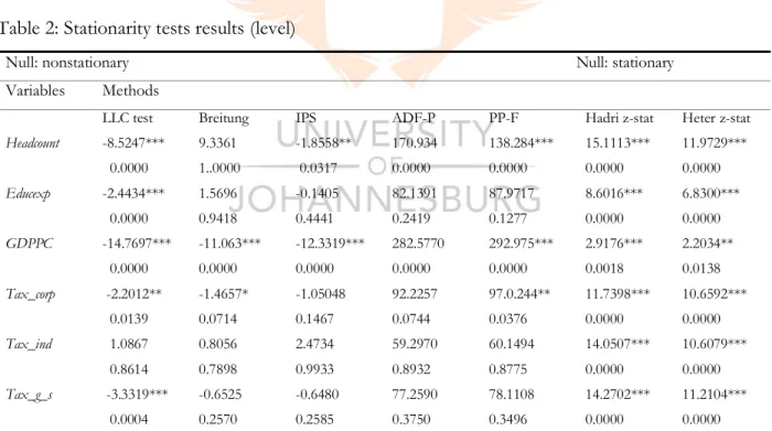
Table2: Stationarity tests results (level)………33
Table3: Stationarity tests results (First Difference)………...34
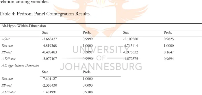
Table4: Pedroni Panel Cointegration Results………...35
Table5: Kao Panel Cointegration Results………...35
Table6: Johansen Fisher Panel Cointegration Results………..36
Table7: Results of FMOLS and DOLS………38
Table8: PMG Results………..39
1
CHAPTER 1: INTRODUCTION
This chapter is structured as follows: Section one deals with the background and problem statement of this research. Section two presents the research motivation while section three provides its contribution to the literature. Section four deals with the research questions and section five presents the importance of the dissertation. Finally, section six provides the structure of the minor dissertation. 1.1 Background and problem statement
The world economy has made considerable improvement over the last two decades in raising the living standards of the poorest. In 1990, about 37% of the global population or 2 billion people, lived below the global poverty line of $1.90 per day. PovcalNet database reveals that in 2013, the period for which the most recent international poverty estimates are available, the amount of those living in extreme poverty had decreased above 60% (766 million people). In the same period, the percentage of the world population living in extreme poverty reduced rapidly to 11% from 37%. The Millenium Development Goals (MDG) of reducing the amount of the extremely poor by half in developing economies from 1990 to 2015 was met in 2010. This is five years ahead of time. Despite this remarkable progress, recent World Bank estimates show that 770 million people were extremely poor in 2013. Ending extreme poverty is a key objective of the global development community. However, eradicating poverty in all its forms is the main and first of the seventeen Sustainable Developemnt Goals (SDG) adopted by the United Nations, and the World Bank has set a main objective of alleviating the rate of the extremely poor at 3% by 2030 (Castañeda et al. 2018).
Castañeda et al. (2016) show that the picture of poverty in developing countries is largely young and rural; 75% of the moderate poor (those who live between $1.90 as the minimum international poverty line and $3.10 as the maximum) live in rural zones as do 80% of the extremely poor (those below $1.90). Almost 60% of the extremely poor reside in households with three or more children, and above 45% of the extremely poor are less 15 years old. The question is whether the continuous persistence of poverty in developing countries is about the implementation of policies for poverty alleviation or nationally raising the required revenue.
Raising sufficient revenue to finance government spending is the main objective of the tax structure of any government in developing countries. As a legal structure, a tax system governs the implementation of the different types of tax such as tax on income, trade tax, consumption tax and social welfare. Governments determine the tax rate and the composition of their taxes. The optimal
2 taxation theory opted for the tax system that maximises social welfare (Diamond and Mirrlees, 1971; Atkinson and Stiglitz, 1976; Saez, 2010; and Maina, 2017). Although recognising the principle of maximising social welfare through a taxation system, developing countries still face significant challenges in collecting revenues to finance their developmental policies (Musgrave and Thin, 1948). This is due to weak tax systems which reduces government’s capacity to offer social services to the poor.
1.2 Motivation for this research
Given the fact that poverty constitutes a challenge for developed and developing countries, scholars (Nyamongo and Schoeman, (2007) and; Lustig and Higgins (2016), find that progressive taxation is more preferable in reducing poverty than regressive taxation due to its efficacy in redistributing revenue in developing countries. In this context the rich are taxed at the highest marginal rates. Therefore, the tax revenue generated through progressive taxation is redistributed to those living below the poverty line (PL). This argument seems specifically effective for a country with high levels of inequality such as South Africa.
In comparison to the above argument, Musgrave and Musgrave, (1989) and Djankov et al. (2010) claim that despite the effectiveness of progressive taxation in alleviating poverty through redistribution, it discourages the incentive to work more in a bid to save more as the marginal tax rate rises with income. This may decrease economic growth as people opt for working less and spending more time in leisure because of higher marginal tax rates.
Most studies (see for example Maina, 2017; Keen 2008) find that decreasing a regressive tax could be beneficial to the poor who benefit for nonzero-rated products in developing countries. Studies confirmed that first, a reduced value added tax (VAT) rate gives more disposable income to consumers who buy goods on which VAT is levied. This increase welfare through purchasing power and reduces poverty. Second, the increased disposable income from the reduced VAT available to consumers may be saved.
Increased savings lead to more money in the financial system which may be channelled into profitable investment programmes. This leads to higher economic growth and poverty alleviation. Third, reduced VAT increases the demand for products through which VAT is levied. This higher demand increases production which could lead to the need for more labour, which decreases unemployment and reduces poverty. Other researchers (Keen, 2003) show that a rise in VAT does not necessarily
3 lead to poverty alleviation, because of the economic theory which implies that indirect taxes usually constitute a load for poor households, and that zero-rating of certain taxable goods consumed by the poor would have small fiscal effect.
In light of the uncertainty over which tax design (direct or indirect taxes) affects poverty, it is therefore critical to analyse the effect of direct and indirect taxes on poverty in developing countries. It appears that while some researchers demonstrate that direct taxes such as corporate income tax and personal income tax decrease poverty (Schoeman, 2007), others such as Maina, (2017) show that indirect taxes such as VAT constitute a key tool in poverty alleviation in developing economies. The absence of consensus on this topic is the motivation for our research. Knowing the determining factors that reduce poverty is important and, in this context, tax design needs to be examined in order to find out whether it is a key instrument in alleviating poverty in developing countries.
1.3 Contribution to the literature
There is little research that analyses the link between taxes and poverty in developing countries. Salottia and Trecroci (2018), investigates the distributional impact of fiscal policy on inequality and poverty by employing data on a panel of 22 developed economies from 1970 to 2010. Investigating this relationship, they use Fixed Effect (FE), Random Effect (RE) and Generalized Method of Moments (GMM), combined with inequality data from the Standardized World Income Inequality Database (SWIID) and the Atkinson and Morelli dataset (2011). Furthermore, to measure poverty, the proportion of household living under 60% of the median equalised disposable income of the country as computed by Atkinson and Morelli (2011), were considered as poor. It has been found that the percentage of people living below this threshold has a negative link with fiscal instruments.
Salottia and Trecroci (2018) also discovered that in developed contries government expenditure on education exerts a negative and significant impacts on reducing poverty through redistribution of revenue. The limitation of their study is as follows: firstly, data on poverty is not accessible for every year in many cases. There are no data on poverty for countries such as Greece, Belgium, Ireland, Denmark, Iceland, Austria and New Zealand (Salottia & Trecroci, 2018). We conclude that their results may lead to bias. Secondly, the econometric approach (FE, RE and GMM) applied in their study is limited in assessing the long run relationship between taxes and poverty. Thirdly, they use 60% national median equivalised disposable income express by national currency as a poverty threshold. Therefore, household living under this threshold is regarded as poor despite this measure being used as a key indicator for eradication of poverty in the European Union until the adoption of
4 Europe 2020. This hides considerable variation across member states as it is computed using a weighted average national results which are limited given that these results are not a direct measure of poverty.
Contrary to the above authors, this study assesses: (i) the link between taxes and poverty using the data from a panel of 37 developing countries from 1996 to 2015. This is crucial as the main Sustainable Development Goal is to eradicate poverty by 2030. Therefore, policymakers need appropriate and specific policy recommendations adapted to the realities of developing countries. This differs from Salottia and Trecroci (2018) who use 22 developed countries as a spatial contribution. (ii), To estimate poverty, we used Headcount as a direct measure of poverty or incidence of poverty. The advantage of poverty incidence (headcount) is that despite the critique developed by Sen (1976) in Econometrica, this measure remains the most widely used, because of its simplicity.
In addition, Ravallion (1996) states that for a subject of such public interest as poverty measurement, formulae of other indexes such as poverty gap (PG), squared poverty gap (SPG), etc. may be hard to understand. To avoid overestimation or underestimation of the effect of taxes on poverty, this study uses the latest global poverty line of $1.90 per day in 2011 from Povcalnet which is the most recent dataset from the World Bank. (iii) Compared to the above study which uses FE, RE and GMM to control for endogeneity, the main contribution of this study is that we use panel cointegration technique to investigate the long run impact of direct and indirect taxes on poverty for 37 developing economies from 1996-2015.
The advantage of Panel Cointegration is that it allows us to examine the long term relationship among variables while letting the short term dynamic change between variables. However, Levine Lin and Chu (LLC) (2002), Im Pesaran Shin (IPS) (2003), Hadri (2000), Maddala and Wu (1999) and Breitung (2000) Panel Unit Root techniques are used to test for the unit root in each series as a precondition while Pedroni, Kao and Johansen-Fisher panel cointegration models are employed to test for the existence of cointegration among variables. To deal with serial correlation and endogeneity, this study applies Fully Modify Ordinary Least Squares (FMOLS) and Dynamic Ordinary Least Squares (DOLS) while Pooled Mean Group (PMG) is used to control for heterogeneity. Finally, we use the Dumitriscu-Hurlin for the causality test between variables.
5 1.4 Research questions
In order to investigate the association between taxes and poverty, this thesis will respond to the following questions:
- Is there a long run relation between direct and indirect taxes and poverty in developing
countries?
- Are direct or indirect taxes effective in alleviating poverty in developing economies?
The response to the first question requires an application of the long run model for taxes and poverty employing panel cointegration.
To provide an answer for the second question, poverty will be regressed against taxes (taxes on goods and services, corporate income tax and personal income tax) and the control variables (GDP per capita and public spending on education).
1.5 Importance of the dissertation
Poverty is a common problem in developing countries. However, its reduction depends on the tax system of each country. This research is expected to ameliorate the understanding of the relationship between tax design and poverty reduction in developing economies. This is of considerable importance to scholars and policymakers, given that it extends the empirical literature on the subject and could promote social stability for developing countries.
This research highlights the importance of direct and indirect taxes in reducing poverty and the urgent need for developing countries policymakers to act and appropriate the full gains (knowledge) of the link between direct and indirect and poverty measurement. Maina (2017) shows that there is a global tendency of increasing VAT (indirect tax) as a percentage of total public revenue. This is due to two reasons: first, the challenge to tax individuals and companies, given the increased mobility of capital and labour. Second, while indirect taxes (because they are levied on consumption) impact a large number of people, personal income tax (PIT), which a direct tax, will impact a small number of people. It is envisaged that the results of this research could be important to policymakers in the attempt to alleviate poverty through tax design.
1.6 Structure of dissertation
This study is set out as follows. Chapter 2 describes poverty and taxes in developing countries. Chapter 3 provides an empirical review of the relationship between direct and indirect taxes and poverty.
6 Chapter 4 provides a brief explanation on data used in this dissertation and describes the methodology employed ‘’panel cointegration’’. Chapter 5 presents the empirical findings of the study. Chapter 6 describes the conclusion and some policy recommendations.
7
CHAPTER 2. POVERTY AND TAXES IN DEVELOPING COUNTRIES
This chapter consists of two sections: Section 1 describes poverty in developing countries and section 2 presents taxes and poverty in developing countries.
2. 1 Poverty trend in developing countries
Poverty is a main challenge on the global agenda. In 1990, the main Millenium Development Goal was to halve extreme poverty rates by the year 2015. This goal has moved to Sustainable Development Goals (SDG). SDGs were adopted in 2015 by global leaders for the purpose of ending poverty by 2030 as a main goal. In addition, the World Bank has set two main objectives that are in alignment with the SDGs in eliminating extreme poverty by 2030, and promoting shared prosperity (Ferreira et al., 2015). Furthermore, development policies for any nation should be focused on ending absolute poverty, which demands both policies to redistribute income mobilised and economic growth (Bourguignon, 2004).
Over the past three decades, PovcalNet’s data shows a general decrease in absolute poverty in developing countries. However, in only few countries poverty in 1981 was higher than in 2010: these incorporate some countries in Sub-Saharan Africa, Eastern Europe and Central Asia, and a few in Latin America and the Caribbean. In the 2000s, poverty reduction was more generalised except for 8 out of 121 economies (five in Sub-Saharan Africa) in which poverty rose between 1999 and 2010. This data reveals that a percentage of the population living with less than $1.25 per day in the developing countries fell to 20.8% in 2010 from 52% in 1981. This indicates a downward trend of around 1 point per year. This is a period where extreme poverty was decreased drastically in a short run. However, this remarkable result must be put into perspective. (i), While four out of ten people have per capita consumption levels of less than $2 a day, one of every five people still lives in extreme poverty in the developing countries, using $1.25 per day. (ii), the rapid economic growth of China is key to this remarkable result. Excluding China, poverty reduction is less significant. Excluding China, it is clear that developing economies could achieve the MDG for poverty alleviation in 2015.
Using $1.25 a day as a poverty line (PL), the extreme poverty rate of each developing economy decreased to 19% in 2010 from 29.5% in 1981, which indicates a decrease of about a third of a point per year. This is less significant compared to one point per year of the global poverty rate. In comparison to the 1990s where poverty alleviation for a typical developing economy was around 1 point per year, poverty fell drastically between 2002 and 2008. The reduction in poverty becomes less
8 surprising when employing higher PLs. However, the incidence of poverty using $1.25 as a PL decreased 60% from 1981 to 2010, and fell 41% when employing $2 PL and 20% with the $4 PL. In fact, the MDG goal of reducing poverty by half ($1.25 per day) from the value in 1990 was already met in 2010, while the evaluation is non-identical when employing the $2 PL; compared to the value of 1990, poverty incidence in 2010 was around two-thirds.
Figure 1 plots poverty rates for developing economies in full and for six regions using $1.90 per day as PL. However, the graph shows that for all the developing world the rate of poverty reduced to 13% in 2013 from 54.7% in 1981. According to the estimation, it is going to decrease further to 11.9% in 2015. Despite this progress in poverty alleviation, Figure 1 also reveals that there are still vast regional discrepancies on the levels of progress in combating poverty at the global level. In the same context, Ravallion (2011) also noticed that that progress in combating poverty has been unequal over time and space. Furthermore, the comparison of progress in poverty alleviation between the six regions from 1981 to 2015 also indicates that there was a noticeable re-ranking. The striking reversal took place in the 1980s and 1990s. For instance, in 1981 the region with the higher poverty rate was the East Asia Pacific (EAP) at 80.5 %, followed by SA at 54.5% and Sub-Saharan Africa (SSA) at 49.2%. During the 1980s and early 1990s, The EAP had considerable number of extremely poor. However, by the early 1990s, SSA became the poorest region, despite a decrease in the rate of poverty during 2000, while the EAP recorded a pronounced fall in poverty rates. From 1981 to 2015, EAP recorded a considerable reduction in the poverty rate to less than 10% in 2011 from 80.5% in 1981 and is estimated to be less than 5% in 2015.
9 Figure 1: Regional Dynamics of poverty
Source: World Bank (2016)
Despite the downward trends observed in poverty in Fig. 1, regional disparities and poverty remain a challenge in developing economies. In order to eradicate this poverty by 2030, policymakers opt for taxation systems as a tool for eliminating poverty in developing economies. It is important to note that when investigating the effect of tax systems on poverty, it is necessary to distinguish between cash transfers (direct effect) from the non-cash transfers (indirect effect) received in the form of free public services in health and education. However, the effect of government expenditure on poverty also depends on the way it is financed (McKay, 2004). Direct taxes such PIT are considered to have negligeable effects on poverty, either because they are outside the direct tax system, or because households living below the poverty line are exempt. In most developing economies, a large proportion of tax revenue comes from VAT, which is an indirect tax. For example, around 60% of tax revenue comes from VAT in Latin America, compared to 40% in OECD economies (Goni, Lopez, & Serven, 2011). It is clear that indirect taxes can raise the poverty rate by increasing the prices of goods and services consumed by the poor. At the same time, monetary financing of public expenditure can also lead to higher inflation, which in turn has an adverse effect on poverty (Easterly & Fischer, 2001).
10 2. 2 Taxes and poverty in developing countries
Studies (OECD, 2008; IMF, 2014) demonstrate that fiscal instruments play an important role in reducing a country’s poverty. However, public spending for provision of fundamental goods and services to lower income earners redistributes income and alleviates poverty. Given the global poverty rate, the role of progressive and regressive taxation in alleviating poverty becomes critical. Taxation is a key policy instrument in poverty reduction. Its capacity in affecting poverty alleviation has been broadly investigated. Scholars such as Okner, (1975) broadly debated whether taxation systems affects poverty positively or negatively.
In fact, taxes determine the disposable income available for household consumption, and thus affect poverty. However, disposable income does not take into consideration indirect taxes or the consumption tax (Karanfil & Ozkaya, 2013). This creates a limitation when using only disposable income in studying tax burdens and poverty, or income distribution. The efficacy of taxes in redistribution has been debated for years. Scholars such as Bird and Zolt, 2005, and Chu et al., 2000 demonstrated that the impact of taxes on poverty is insignificant in developing economies. In the following sections, we focus firstly on the impact of indirect taxes on poverty and secondly on the effect of direct taxes on poverty.
2.2.1 Effect of indirect taxes on poverty in developing countries
The World Bank, (2006) stated that developing economies are characterised by low levels of taxation, heavy reliance on regressive revenue instruments, and low coverage and benefit levels of transfer programmes. This limits the redistributive effect of taxation systems in developing countries. According to Baltagi et al., (2012), while the average tax ratios for developed countries is over 30% of GDP, that of developing countries (without emerging Europe economies) is between 15%–20 % of GDP. Tax mobilisation is not only lower but also more regressive than in developed economies. The challenges in applying more progressive taxation are linked to the larger size of informal sectors and higher degrees of self-employment. This limits the ability of the tax authorities to control the assets and income of taxpayers.
On the public spending side, in several developing countries public expenditure on social programmes is low, and contributions to social insurance programmes are reserved for public sector workers and high-income employees in the formal sector. All these factors lead to low redistributive effect of the
11 fiscal instrument on poverty in developing economies. Bahl and Bird (2008) show that while the share of personal income tax and excise duty has decreased, that of corporate income tax and VAT in OECD countries has increased. However, in developing economies, indirect taxes such as VAT play a key role.
Case of negative effect indirect taxes on poverty
Corriea (2007) demonstrated that a constant rate of tax on consumption, which is indirect taxes will ameliorate equity and standard of living, without transferring cash to the extremely poor household. He concludes that the more indirect taxes, such as consumption taxes, contribute to the public revenue, the more are the impacts on efficiency and living standards of the poor, through the provision of public goods such as education, health, public roads etc. In fact, this argument of consumption tax differs from the usual argument of indirect taxes (consumption taxes) as regressive.
Case of Positive effect of indirect taxes on poverty
Some studies (see for instance, Karanfil & Ozkaya, (2013)) have investigated the regressivity of indirect taxes on poverty. The results show that indirect taxes have a significant positive long-run effect on poverty. In other words, an increase in indirect taxes raises poverty. This means that a rise in indirect taxes reduces the purchasing power and the welfare of the poor. However, there is a heavy reliance on indirect taxes by policymakers to increase public revenue, given that they are easy to mobilise at a reduced political cost.
In comparison with progressive taxation, which is considered as equitable, – the share of income spent in taxes increases as incomes increase, and when the direct taxes are progressive, regressive taxation is regarded as inequitable. In other words, because the poor and the rich pay the same tax rate when buying goods and services, lower income earners spend a larger amount of their income on goods and services taxes (indirect taxes), as they consume more than they save compared to the rich. For example, consider two individuals paying R10 as the tax rate on tobacco products; one earns R100 and the other R1000. This illustration indicates that lower income earners spend more on tax, as R10 is 10% (10/100) of his income, compared to the higher income earners who pay only 1% (10/1000) (Esmaeel, 2013).
12 Case of Zero-rating and poverty
Low tax rates combined with high tax rate on luxury goods and exemptions on basic commodities may lead to the progressivity of consumption taxes. Studies (see for example, Casale, 2012; Saez, 2010 ;Karingi, et al., 2004) indicate that taxes on commodities can be employed to complement direct taxes in redistributing income in the short term. It has been found that zero-rating of some specified basic goods, mostly used by poor (basic food items and paraffin), benefits the poor. However, excise tax imposed on luxury goods such as watches, yachts, private jet planes, jewellery and expensive cars has the impact of raising equity. In another words, higher income earners are those who consume luxury goods and services and therefore, they pay the taxes. The revenue generated from those taxes can be used for the provision of public utilities to poor households. In Uganda for instance, zero-rating on certain goods has little fiscal effect on poverty. The argument is that an increase in tax burden through progressivity of VAT can be translated into appropriate service delivery for poor. In this context, non-exempted items are taxed more in order to avoid public revenue erosion.
2.2.2 Effect of direct taxes on poverty in developing countries
A tax system is a combination of public expenditure and tax policies in a legal and administrative framework. However, each element affects negatively or positively on poverty. A mixture of these policies determines who pays what, and how it may affect significantly poor households. In fact, a taxation system is rarely neutral; quite the contrary. In order to understand this, some concepts related to equity and efficiency and the characteristics of regressive and progressive taxation need to be grasped. A tax system is considered efficient if it causes interference in economic decisions that would be made if the tax did not exist. However, horizontal equity is when equals (those who have the same income) have the same fiscal treatment, while vertical equity means that non-equals should have different fiscal treatment. As with equity, a tax system is progressive when it is built on the theory that the more the income, the more tax should be paid. In other words, a taxation system is progressive if the higher income group pays more tax than the poor. It is regressive if the opposite is true. (Itriago, 2011). However, in this dissertation, direct taxes may impact poverty through PIT or CIT.
Personal Income tax and poverty
It is clear that direct taxes such as PIT are equitable because they are progressive by nature. This means that the rich, given that they save more than they consume, pay more tax than the poor. Then the revenue generated from those taxes is utilized, whether for cash transfers or for providing social
13 facilities such as food, housing facilities, clothing, education, healthcare etc. for the poor section of societies. (Esmaeel, 2013). Despite the fact that progressive taxation is more preferred to reduce poverty through income redistribution, it may discourage thework incentive, which impedes productivity and economic growth. (Djankov et al., 2010).
In developing countries, the effect of direct tax on poverty is negligeable due to following reasons: (i) the proportion of PIT is insignificant in developing countries, because it is levied in the formal sector. In most developing economies, the growth of the informal sector is a key factor that impedes the efficacy of PIT. It is likely that the informal sector reduces a considerable proportion of the tax base as it grows. Due to the lack of administrative capacity to identify employees or workers in the informal sector, the low, middle- and high-income earners are exempted from taxes. This reduces the role of a redistributive policy in developing world. (ii) the ineffectiveness of tax administration limits the capacity for raising sufficient public revenue though PIT. This is due to the lack of skill and resources to deal with income tax administration. (iii) poor governance and corruption render ineffective not only redistributiion effects but also the tax system. This limits the impact of redistributive policies. (Robinson, 2003; Kayaga, 2007; Bird & Zolt, 2005).
Corporate Income Tax and poverty
CIT can influence poverty in several dimensions. In this section, we discuss a few of them. The case of Indonesia in 2008 shows that the effect of CIT on poverty in developing countries depends on how large the extent of impact of shocks is on changing factors such as income and price levels in the economy. In fact, the extent to which the factors of income and price changes may impact headcount (incidence of poverty) depends on the sources of income and consumption patterns of people living in poverty. It may also depend on the sensitivity of PL in response to the change in prices.
Indonesia’s case shows that CIT reduces poverty in the sense that first, a drop in the CIT decreases the prices of goods, wage raises and returns on capital. This entices investments and promote economic growth through job creation. Secondly, a reduction in prices of goods increases the buying power of the poor and keeps the PL at a low level, while rises in incomes increases the ability of the poor to consume more. This increases their welfare and reduces their poverty level. (Dartanto, 2012). Pakistan’s case reveals that taking into account tax evasion, CIT is ineffective in reducing poverty. A rise in CIT drastically decreases the capital formation rate, by decreasing the marginal product of labour, which leads to a negative income impact on all categories of society, specifically those living
14 in extreme poverty. It is important to note that the poor are the most affected, given that the largest part of their income originates fromtheir labour (Feltenstein,2017).
Education and poverty
A rise in coverage and better targeting of social policies was a sign of improvement in the 1990s. The actual conditional cash transfer programmes (CCTs) is a key constituent in ameliorating the distributive effect of government expenditure in developing economies. This programme transfers income to poor households, conditional on households investing in their children's human capital, such as education, health and nutrition. CCTs have been applied on a small scale in several regions of developing economies such as Sub-Saharan Africa (SSA) and Latine America Caribbean (LAC). (Garcia and Moore, 2012)
Education is important for ending poverty and for economic development. There is no economic development without education. A good education system not only improves economic development, but also productivity, and generates personal income per capita. Its impact is seen at the micro level of individual families whose combination makes up a nation.
15
CHAPTER 3: LITERATURE REVIEW
A literature review is key to any academic study. The need to discover what has been done in the field before initiating any study should not be neglected. This chapter offers an overview of the existing empirical literature on the effect of direct and indirect taxes on poverty in developing economies, and how this study contributes to the literature.
3.1 Empirical review
The empirical literature on tax design and poverty in developed and developing economies is well established. To investigate the effect of direct and indirect taxes on poverty in developing economies, this study focuses on redistributive taxation channels.
García and Giraldo (2018) use a Computable General Equilibrium (CGE) microsimulation method, which is a nonlinear model, to evaluate the effect of tax policy changes on growth, welfare and income distribution in Colombia. They employ household survey data. Their findings show that indirect taxes constitute a key instrument for the policymakers in Colombia, due to their effectiveness in collecting revenue and their decreased rate of evasion. It was also found that by applying zero tax on the poor, and reducing the tax burden of enterprises, investment can be stimulated. This may lead to economic growth and poverty alleviation. Their findings have shown that reduced indirect taxes such VAT give more disposable income to the consumers who buy products on which VAT is levied. This increases welfare through purchasing power and reduces poverty. Their study concludes that the best tax design is the one that compensate income to lower income earners.
Ahmed et al. (2010) assess Pakistan’s tax reform and its effect on poverty and inequality using a CGE microsimulation technique. The results demonstrated that due to the structure of income earners in most developing economies, redistribution and a progressive tax system are hardly achieved. For instance, in Pakistan, more than 30% of people live under PL and 68% reside in rural zones. This makes the possibility of direct taxes less attractive. However, to meet public spending needs, taxes on goods and services (indirect taxes) account for a large share of total revenue given that they are hard to evade. Furthermore, it is concluded that an increase in taxes on goods and services leads to a fall in consumption levels of households. In fact, this is an indication of a decrease in wages, which in turn increases the national poverty incidence (Headcount) by 4.7%.
Amir, Adjaye and Ducpham, (2013) analyse the effect of the Indonesian income tax reform employing a CGE study from 1980 to 2008. This is done using a Social Accounting Matrix combined with the
16 National Input-Output Table. They also indicate that the reductions in PIT and corporate income tax (CIT) boost the economy. Their findings also show that their tax design leads to a small decrease in headcount (poverty incidence).
Feltenstein et al. (2017) investigate the poverty implication of alternative tax reform using a CGE microsimulation model that include the endogeneity of tax evasion. Their results demonstrate that an equal yield rise in corporate tax and sales rates produce different effects on poverty and consumption. They show that their findings should be taken with caution, due to the omission of sales and personal income tax evasion. Their findings also reveal that a rise to 45% from 35% in CIT leads to 21.1% of tax to Gross Domestic Product (GDP) ratio, which is specifically what has been collected by the 17% sales tax rate.
Immervoll et al. (2006) study the direct effect of tax burden and benefit payment s on poverty and inequality using the BRAHMS approach. This is a new tax-benefit microsimulation model, which gives entire information on tax paid and benefits received by households in a sample of the Brazilian total population. In addition, this study employs the 2003 PNAD dataset (National Household Survey) in Brazil. Their findings have shown that PIT renders the taxation system an ineffective redistributive instrument. For future policy recommendations, they suggest that it would be advisable to include other instruments in this simulation model, specifically non cash transfers such as education and health, and indirect taxes.
Okidi and Ssewanyana (2008) investigate the impact of tax system on poverty using UGATAX technique (a microsimulation of the Uganda Tax System) from 1999 to 2003. This technique captures direct and indirect taxes using a household as the unit of study. The study was implemented as UNHS I, Uganda national household survey of 1999/00. The main objective of UGATAX is to investigate the tax reform in the context of public revenue gain, the distributive effect and the impact on households living in poverty. Their findings support the argument that first; an increase in VAT from 17% to 20% holding other taxes constant will raise the tax burden of those below the PL. Each of the poor will pay an additional 243 Shilings due to an increase in VAT. But compared to the poor, non-poor will continue to pay more. Okidi and Ssewanyana (2008) advise to maintain the progressivity of VAT as an effective scope for upcoming moves in the tax structure. However, the restricted assumption is that a rise in tax burden will be converted into viable service delivery. Second, exemption (zero-rating) of most taxable items consumed by the poor would have small fiscal effect. In other words, the share of revenue forgone from the zero-rating is small. This policy was motivated
17 by a desire to initiate more progressivity in VAT, which is the principal component of indirect taxes. This indicates that due to their assumption of avoiding the erosion of revenue, non-exempted goods and services need to be highly taxed.
Maina (2017) tests the effect of consumption taxes on poverty and inequality in Kenya using two OLS models; first to show how consumption taxes effect inequality. Second to assess the impact of consumption taxes on the GDP per capita, which is a proxy of poverty. Maina (2017) uses 45 observations starting from 1970 to 2014. He also recommends that policymakers use fiscal policy as a tool to redistribute wealth. His study concludes that consumption taxes are regressive. The study also suggests the use of differentiated rate targeting the of poor. This means that lower taxation rates need to be applied on goods which the poor spend more of their income. By reducing indirect taxes such as taxes on goods and services may increase the purchasing power of the poor. This will increase their welfare and reduce their poverty.
Scholars such as Anderson et al. (2018) assess how government spending affects poverty using Cross-country Meta Regression Analysis (OLS, GMM, FE and RE and 2 SLS) to show a variety of findings from the linear to the nonlinear model. Their arguments reveal that fiscal instruments play a limited redistributive role in emerging economies, because: the less progressivity in a tax system, the lower the level of taxation and spending and the lower level of governance. They also find that compared to the estimates derived from 2 SLS, FE, RE and GMM, OLS estimates show that the link between poverty and public spending employing OLS is more negative.
Higgins and Lustig (2016) assess the relationship between poverty and taxes by comparing transfers and poverty before and after taxes. Their findings demonstrate that these comparisons combined with the measurement of progressivity and horizontal equity, may not to take into account a critical element: that a percentage of people in poverty become more poor (or those above the PL become poor) through the transfer and tax system. Their studies demonstrate with data that from 17 emerging economies out of 15, the tax system is progressive and decrease poverty through redistribution but in 10 of these emerging economies, one-quarter of people living in poverty receive less in transfers than the taxes they pay.
They called it ‘’fiscal impoverishment’’(FI). After measuring the fiscal gain of poor (FGP), they show that poverty gap changes may be decomposed into FI and FGP.
18 Using a comparative fiscal incidence study to investigate the effect of fiscal policy on poverty and inequality for 29 developing countries for 2010, Lustig (2017) employs three measures to assess the impact of tax systems on poverty: headcount, market income of the poor (which leads the poor to be net taxpayers to the tax system in cash terms), and fiscal impoverishment (FI). Their findings show that the share of social expenditure to GDP (redistributive effort) in each economy is firstly the key factor for fiscal redistribution, and the extent to which direct taxes are targeted to the rich and transfers are targeted to the poor. Lustig’s (2017) results also support redistribution through public goods. For instance, the more these public services are used by the poor the more middle income classes and the rich are given poor quality public services. In this context, the middle classes and the rich may be resistant to paying the taxes required to ameliorate the quality of the public services if they move out of these system. Finally, the key finding in this study is that there is no confirmation of the “Robin Hood paradox” that redistribution from the rich to the poor increases inequality. This means that the redistribution policy reduces inequality.
Generally, there are very limited number of studies analysing the effect of direct and indirect taxes on poverty in developing countries. Against this above background, this study contributes to the literature by assessing the effect of direct and indirect taxes on poverty in 37 developing countries, using a panel cointegration model from 1996 to 2015. This model is useful in studying the long-run association between our variables. However, as macroeconomic variables are characterised by unit root in a long period (Nelson & Plosser, 1982), the precondition of this model is to test that all series are stationary. However, this shows that the results would be biased without panel unit root tests. This is contrary to other studies, which do not take into consideration the non-stationarity issue in the model. For example, Salottia and Trecroci (2018), who employ FE, RE and GMM and others (see for instance Lustig, 2017; Higgins & Lustig, 2016; Maina, 2017; Okidi & Ssewanyana, 2008; Immervoll et al. 2006; Amir, Adjaye & Ducpham 2013), who use different techniques such as a tax-benefit microsimulation model, CGE analysis, OLS, comparative fiscal incidence analysis etc., to test the link between taxes and poverty.
Contrary to the Salottia and Trecroci (2018), which tests the effects of fiscal policy on poverty for 22 developed economies, we use 37 developing economies to test this link. The argument is that given the higher the rate of poverty incidence in developing countries, policymakers need a suitable taxation system which reduces poverty in the context of developing countries. In addition, due to the
19 importance of the concept of poverty by the public, our study uses the most used and simple direct poverty measure, the “Headcount ratio,”. This contrasts with Lustig (2017) and Salottia and Trecroci (2018). The former uses $1.25 per day in 2005 as a PL, while the latter uses the poverty measure developed by Atkinson and Morelli (2011). These authors regarded the proportion of households living below 60% of the median equivalised disposable income of the country as poor.
20
CHAPTER 4: METHODOLOGY AND DATA
This chapter analyses data and explains econometric techniques applied to investigate the effect of direct and indirect taxes on poverty in developing countries. It is structured as follows: Section 4.1 presents the data analysis while section 4.2 provides the model specification of poverty. Section 4.3 deals with estimation techniques.
4.1. Data analysis
4.1.1 Data collection and their expected signs
To investigate the effect of direct and indirect taxes on poverty, this research used a sample of 37 developing economies from 1996 to 2015. This sample was a rational choice for two reasons; first, it consists of developing countries which experience higher level of poverty. According to the World Bank, these countries are ranked as countries with low levels of total tax revenue as a percentage of their GDP. Second, the time period for this analysis begins from 1995, as it was the year for which the dataset was available for many developing economies. (See Appendix 1 for the list of developing countries).
The Taxes dataset (%GDP) employed in this research were obtained from UNU WIBER 2018 (GRD) while poverty incidence (Headcount) was obtained from the Povcalnet dataset. However, the data on GDP per capita and public expenditure on education (%GDP) were obtained from WBI. Due to the missing data issues observed in our sample, we used an interpolation technique to fill the gap in our variables.
However, while our dependent variable is the incidence of poverty (Headcount), there are several regressors such as CIT (tax_corp), PIT (tax_indiv) and tax on goods and services (tax_g_s). Public expenditure on education and GDP per capita were used as our control variables. The choice of these variables was based on the literature in the Chapter 2 literature review. Most scholars (see for instance Bird and Zolt 2005; Maina 2017), show that corporate tax (direct taxes) and tax on goods and services which include VAT (indirect taxes), are key factors in alleviating poverty in developing economies. These scholars found that poverty reduces as tax on goods and services and corporate increase. Therefore, the expected signs of tax on goods and services and corporate tax are anticipated to be negative. However, the marginal effect of personal income tax is anticipated to be positive or negative in developing economies. This means that in most cases personal income tax does not play a key role in reducing poverty in developing economies.
21 4.1.2 Descriptive statistics
Before analysing whether the direct and indirect taxes have impacted poverty in developing economies, we need to examine the distribution and the patterns of our dataset. There are 740 observations for 37 developing economies from 1996 to 2015.
Table: 1. describes the summary statistics focusing only on the means of independent and dependent variables employed in our thesis. The results from Table 1 reveal that on average, the incidence of poverty (Headcount) is 0.20 in developing countries with the standard deviation of 0.22. In addition, CIT has a mean of 2.45 in developing countries. A similar trend is observed on PIT where the mean is 2.48 while TGS remains high at 8.4 in developing countries. It was also found that 4.27, 4 and 9 represent the means of government spending on education, the GDP per capita, and the unemployment rate, respectively.
Table 1: Descriptive statistics
Var. Obs. Mean Stand. Dev.
Headcount 740 0.20 0.22 Tax_corp 704 2.45 1.32 Tax_ind 712 2.48 2.09 Tax_g_s 729 8.09 3.47 Educexp 655 4.27 1.86 GDPpc 740 3.01 4.02
Fig.2 below plots the developing economies headcount, tax on goods and services, personal income tax and corporate tax over the period 1996-2015. Our data confirms that poverty incidence shows a moderate upward trend from 1996 to 1999, which is followed by a downward trend from 1999 to 2015. However, TGS which is the highest contributor in developing economies, has an increasing trend, while PIT and CIT show a moderate increase from 1996 to 2015. As shown in Fig.2, this increase in tax on goods and services plays an important role in poverty reduction in developing countries from 1996 to 2015.
22 Fig 2. Presents developing economies headcount, tax on goods and services, corporate income tax and personal income tax for the period 1996-2015.
4.2 Model specification
In order to examine whether there is a long run association among our variables, we used an econometric specification incorporating poverty incidence (P), corporate tax (tax_corp), personal income tax (tax_indiv), tax on goods and services (tax_g_s), public expenditure on education (educ_exp) and GDPpc. Based on our research question, a conceptual model (regression functional form) was established where poverty incidence (P) is a function of tax_corp, tax_indiv, tax_g_s, educ_exp, GDPpc and idiosyncratic error term (e).
𝑃𝑖𝑡 = 𝑓(𝑡𝑎𝑥_𝑐𝑜𝑟𝑝𝑖𝑡; 𝑡𝑎𝑥_𝑖𝑛𝑑𝑖𝑡; 𝑡𝑎𝑥_𝑔_𝑠𝑖𝑡; 𝑒𝑑𝑢𝑐_𝑒𝑥𝑝𝑖𝑡; 𝑔𝑑𝑝𝑝𝑐𝑖𝑡; 𝑒𝑖𝑡) (1) Following Salottia and Trecroci (2018), a panel regression of Eq. (1) can be described as follows:
𝑃𝑖𝑡 = 𝛼0+ 𝛼1𝑡𝑎𝑥_𝑐𝑜𝑟𝑝𝑖𝑡+ 𝛼2𝑡𝑎𝑥_𝑖𝑛𝑑𝑖𝑡+ 𝛼3𝑡𝑎𝑥_𝑔_𝑠𝑖𝑡+ 𝛽́𝑗𝑐𝑜𝑛𝑡𝑟𝑜𝑙𝑠𝑖𝑡 + 𝜇𝑖𝑡 (2)
where 𝑃𝑖𝑡 is the poverty indicators (Headcount or incidence of poverty), i stands for country and t represents period of time. The regressors consist of 𝑡𝑎𝑥_𝑖𝑛𝑑𝑖𝑡 (personal income tax), 𝑡𝑎𝑥_𝑐𝑜𝑟𝑝𝑖𝑡
23 (corporate tax) and 𝑡𝑎𝑥_𝑔_𝑠𝑖𝑡 (tax on goods and services). The following control variables were added to complete our model: (i) public expenditure on education (𝑒𝑑𝑢𝑐_𝑒𝑥𝑝𝑖𝑡); (ii) GDP per capita
(𝐺𝐷𝑃𝑝𝑐𝑖𝑡) and 𝑣𝑖 , country-specific fixed effect,𝑢𝑖is an error term. 4.3 Estimation Techniques
Our econometric technique was composed of 5 steps: (i) Panel unit root tests were used to ensure that all variables were in the same order of integration (ii) Panel cointegration tests were employed to test for the presence of cointegration using our variables in their first difference (iii) FMOLS and DOLS were utilised to estimate the long run relationship among variables and to deal with serial correlation and endogeneity issues (iv) PMG was used for robustness checking and to control for any heterogeneity problem (v) the Dumitrescu and Hurlin test was applied to test for the direction of short-run causality.
4.3.1 Panel unit root
According to Nelson and Plosser (1982), macroeconomic series are characterized by unit root when the time period of the sample is long in the panel. Therefore, it is critical to test for the integration order of the series before investigating any long term association. However, panel unit root techniques for all our series were imperative. It is important to note that panel unit root techniques include a multivariate analogue to standard univariate unit root techniques, incorporating KPSS, ADF and PP techniques. The major objective in expanding the application of simple time-series unit root techniques to panel data is to employ the increase in sample size by pooling cross-sectional data to ameliorate the power of the techniques. In this study, five panel unit root techniques were analysed, namely: the LLC (2002), IPS (2003), Hadri (2000), Breitung (2000) and Maddala and Wu (1999) techniques.
A simple technique assumes the series of time on the cross section individuals i = 1, 2,3,4 ..., M over periods of time T are produced for a single i by a simple first-order autoregressive, AR (1), process:
𝑦𝑖𝑡 = (1 − 𝜌𝑖)𝜇𝑖+ 𝜌𝑖𝑦𝑖,𝑡−1+ 𝜀𝑖𝑡 (3) t=1,2, 3, T and i=1,2, 3…, M
Where 𝑦𝑖𝑡 represents the observed i-th individuals over period of time T. Error terms 𝜀𝑖𝑡 are independently and identically distributed (iid) for a unit i at the time periods T. 𝜀𝑖𝑡 describes white
24 noise for a unit i at the periods of time T. 𝜌𝑖= 1 for all i under the null of unit root and Eq. (3) can be described as the Augmented Dickey-Fuller (ADF) specification:
∆𝑦𝑖,𝑡 = 𝛼𝑖 + Φ𝑖𝑦𝑖,𝑡−1+ ∑𝑞𝑖 𝛾𝑖𝑗∆𝑦𝑖,𝑡−𝑗+ 𝜀𝑖,𝑡
𝑗=1 (4)
Where 𝑦𝑖 describes coefficients to be determined (estimated) for the ith individual and 𝜙
𝑖 = (𝜌𝑖− 1),
𝛼 = (1 − 𝜌𝑖), 𝑞𝑖 represents the number of lagged terms for the ith individual Δ𝑦𝑖,𝑡 = 𝑦𝑖,𝑡− 𝑦𝑖,𝑡−1
and all other parameters are as previously defined.
As a first step, this dissertation used a stationarity test to check if the variables incorporated in the model had the same order. To test the integration of order, this study employed stationarity tests established by LLC, IPS (2003), Breitung (2000), Hadri (2000), and Maddala and Wu (1999). From each method, this dissertation assessed for unit root tests in the panel by employing five types of techniques. Based on the ADF technique, the LLC technique is the most employed technique in panel settings.
4.3.1.1 Levin, Lin and Chu (LLC) technique
This panel unit root technique was developed by Levin and Lin (1992) and formalised by Levin, Lin and Chu (2002). This technique allows the time trend, intercept, higher-order autocorrelations and residual variance to vary across the units.
The LLC technique is founded on a pooled panel estimator which assumes a common 𝜙𝑖 = 𝜙 but permits 𝑞𝑖to change across the cross-sectional units. This also demands a common sample size from
the independently generated time series. This technique can be considered as a pooled ADF technique with different lag lengths across the units of the panel. The major disadvantage of this technique is that it imposes a cross-equation restriction on the first-order autocorrelation coefficients. According to LLC, the alternative and null hypothesis are as follows:
𝐻0 ∶ 𝜙1 = 𝜙2 = ⋯ = 𝜙𝑀 = 0 𝐻0 ∶ 𝜙1 = 𝜙2 = ⋯ = 𝜙𝑀 < 0
According to LLC, each cross sectional unit has a unit root under the null hypothesis, while each cross-sectional unit has no unit root under the alternative hypothesis.
25 4.3.1.2 Im, Pesaran and Shin Technique
The IPS (2003) technique is established as taking into account the main limitation of the LLC technique, where it is presumed that all unit AR (1) series have the same autocorrelation coefficient. It permits for individual processes by allowing 𝜙𝑖 to change across the cross-sectional units. This
technique starts by establishing a separate ADF regression for a single cross-sectional unit in Eq. (4). According to IPS, the alternative and null hypothesis are as follows:
𝐻0 ∶ 𝜙𝑖 = 𝜙 = 0 𝑓𝑜𝑟 ∀ 𝑖
𝐻0 ∶ 𝜙𝑖 < 0 𝑓𝑜𝑟 𝑖 = 1,2, … . . , 𝑀1 𝑎𝑛𝑑 𝜙𝑖 = 0 𝑓𝑜𝑟 𝑖 = 𝑀1+ 1,…, 𝑀
According to IPS, all cross-sectional units have a unit root under the null hypothesis while at least one unit is stationary under the alternative. This shows that IPS is different from the LLC technique which assumes that all units have no unit root under the alternative hypothesis. The IPS technique is founded on M independent tests on M cross-sectional units while the LLC technique combines the test statistics. However, the random errors, ℰ𝑖,𝑡, are presumed to be serially correlated with different variances across a single unit of a cross-section, and different serial correlation properties. The key of this technique is founded on a group-mean t-bar statistic where the t-statistics are obtained from a single ADF technique and averaged across the cross-sectional units over time (panels). Under the null hypothesis, the factors of adjustment are employed to standardise the T-bar statistic into a standard normal IPS W-statistic.
4.3.1.3 Hadri technique
The Hadri (2000) panel unit root technique is similar to KPSS unit root technique with the null of stationarity in any of the units in the panel. As KPSS unit root technique, this technique is founded on the residuals obtained from individual OLS regressions of 𝑦𝑖,𝑡 on a constant or a constant and a trend. The statistic test is distributed as standard normal, under the null hypothesis. The error process can be presumed to be heteroskedastic across the cross-sectional units or homoscedastic across the panel. However, this technique presents two Z-statistics. The first Z-statistic is obtained from the LM statistic where the residuals derived from the ADF regression are connected with the homoscedasticity assumption across the panel and the second employs the LM statistic that is heteroscedasticity consistent.
26 4.3.1.4 Breitung technique
Breitung (2000), developed a pooled technique that does not necessitate bias correction factors. This is attained by a relevant variable transformation. The IPS technique loses the power given the bias correction when individual-specific trends are incorporated into the model. Breitung (2000) suggests another unit root test which has more power than the IPS test and can control for the loss of power. The null for this technique assumes a non-stationarity difference in the panel series, while the alternative assumes that the panel series are stationary.
4.3.1.5 Maddala and Wu technique
Compared to the IPS technique based on an asymptotic and parametric test, Choi (2001) and Maddala and Wu (1999) proposed a non-parametric focusing on the Fisher (1932) technique. They incorporated the P-values from the individual stationarity technique. The importance of this technique is that its value is not based on different lag lengths in the individual ADF regressions.
The t-statistic is given by:
𝑃𝑀𝑊 = −2 ∑𝑁𝑖=1𝑙𝑜𝑔𝜋𝑖 (5)
According to MW test, if the t-statistics is continuous: Firstly, the level of significance, π (𝑝 − values 𝑜𝑟 𝑃𝑀𝑊) of the t-statistics is uniformly and independently distributed between [0, 1] under
the null. Secondly, -2 log π has a distribution of 𝑋22. Thirdly, under the null hypothesis,
−2 ∑𝑁𝑖=1𝑙𝑜𝑔𝜋𝑖 has a distribution of 𝑋2𝑁2 where the degree of freedom is described by 2N. The null is non-stationary for each series, i.e. H0: 𝜌𝑖 = 0 for each i. However, not all series are non-stationary
under the alternative hypothesis i.e. H1: 𝜌𝑖 < 0 for i = 1,….., N1 and 𝜌𝑖 = 0 for i = N1 +1,….., N.
4.3.2 Panel Cointegration Technique
After testing for stationarity, the following step is to study the long term link among variables employing the Pedroni (1999), Kao (1999) and Fisher/Johansen cointegration methods. Breitung and Pesaran, (2005) demonstrated that the cointegration technique which controls for the existence of long-term association among integrated variables is a common instrument in the literature.
According to Pedroni, (2004), several techniques have only small impact when applied to single unit time series available after World War II. Because of this issue, it has been found essential to extend the sample by incorporating additional cross-sectional data and investigating cointegration associations in a pooled panel of time series.
27 Furthermore, by employing cointegration techniques, variables need to be measured in levels. Therefore, our technique may be viewed as more precise way for analysing the presence of a long-term association among variables. In the following section, we describe three fundamental panel cointegration techniques: Pedroni (1999, 2004), Kao (1999) and Maddala and Wu (1999).
4.3.2.1 Pedroni Technique
Engle and Granger (1987) established the cointegration technique for individual unit time-series. This technique is founded on the analysis of residuals of the regression employing I (1) variables. For these variables to be cointegrated, the necessary condition is that the residuals should be I (0). However, there is no cointegration if the residuals are I (1) and therefore no long-term equilibrium relationship among the variables. Pedroni (1999) expand the Engle-Granger based on the residuals technique to the panel setting. This technique needs to determine the residuals from the regression of the hypothesised cointegration. Therefore, consider the following regression:
𝑦𝑖𝑡 = 𝛿́𝑖𝑑𝑡+ 𝛽𝑖𝑥𝑖𝑡+ 𝑒𝑖𝑡 (6) where t =1…...T stands for the time period index and i = 1…., N describes the cross-sectional units. The term 𝑑𝑡 contains the deterministic components, which can be explained in three types of specifications. 𝑑𝑡 = 0 when no deterministic trend is incorporated in the equation (6). While 𝑑𝑡 = 1 implies an individual constant trend when 𝑦𝑖𝑡 is modelled, 𝑑𝑡 = (1, 𝑡)′ implies time trend and an
individual constant when 𝑦𝑖𝑡 is modelled. It is important to note that parameter 𝛿𝑖 controls for
deterministic trend and individual specific fixed effects. In addition, the slope coefficients can change across units. 𝑦𝑖𝑡𝑎𝑛𝑑 𝑥𝑖𝑡(variables of interest) are presumed to be I (1) for single cross-sectional
individual i. According to the Engle-Granger technique, error term 𝑒𝑖𝑡 should also be I(1) under the null of no cointegration. From the transformation of the equation (1), we can obtain first the following residuals equation: 𝑒̂𝑖𝑡 = 𝑦𝑖𝑡− 𝛿̂𝑖′𝑑𝑡− 𝛽̂𝑖𝑥𝑖𝑡 and examine if the residuals are I (1) by running an
additional regression for each cross-sectional unit:
𝑒̂𝑖𝑡 = 𝜌𝑖𝑒̂𝑖,𝑡−1+ 𝜇𝑖𝑡 (7)
𝑒̂𝑖𝑡 = 𝜌𝑖𝑒̂𝑖,𝑡−1+ ∑𝑝𝑖 𝜓𝑖𝑡