120
Developing a model for pricing and control the inventory of
perishable products with exponential demand
Mostafa Setak
1*, Nazanin fozooni
1, Hamed daneshvari
11Department of Industrial Engineering, K.N. Toosi University of Technology, Tehran, Iran
[email protected], [email protected], [email protected]
Abstract
Pricing and controlling the inventory of perishable products have key roles in determining the level of profit for those involved in the supply chains. Chain profit can be increased by increasing sales during the product life via the application of pricing strategies, avoiding the loss of value of perishable products over time. In this research, sales profit was maximized by presenting a mathematical model to determine the price change points (using the Hsien function) and the optimal price and order quantity for perishable products with an exponential and price- and time-dependent distributed demand. Due to the complexity of the problem, the solution method used in this study was the genetic algorithm. The analysis of the effect of different parameters and optimal solution results showed that a 2% increment in decay rate would lead to a 10% reduction in profits, and other analyses recommended for managers at the end of the article.
Keywords: pricing, inventory, perishable products, exponential demand.
1- Introduction
Nowadays, the management and control of deteriorating inventories is of special importance in many industrial units. In 2006, the global sales of grocery retail units was more than 1,000 billion, and over one third of this figure was related to deteriorating products such as fruits, vegetables, meat, and dairy (Broekmeulen and Van Donselaar 2009). In today's world, customers look for more diversity, especially in the case of decaying products with limited life spans. This leads to further out-of-date inventories, making the prediction of the demand function more difficult. Also, often in the real world, to control the demand rate, more cost-cutting policies are employed by managers as the product nears its expiration date. Sometimes, depending on the type of product, the deteriorated items are removed from the warehouse. Considering such factors, the issue is more difficult to mathematically model in comparison to modeling the inventory control of non-perishable products. The purpose of is the present study was to propose a mathematical model for determining both the optimum time for changing the price and the optimal price in order to maximize profits. In addition, the issue of pricing and inventory control for perishable products was reviewed. In this research, we are looking for a new approach to simultaneously optimize the price and control the inventory of decay items, where demand is a function of time and sales price. In this study, Decline in the rate of corruption is considered constant.
*Corresponding author
ISSN: 1735-8272, Copyright c 2019 JISE. All rights reserved Journal of Industrial and Systems Engineering
Vol. 12, No. 3, pp. 120- 140 Summer (July) 2019
121
One of the obvious features of this study is that Utilizing pricing strategies and discounting the prices of these products can increase the profitability by increasing sales over the life of the product. Another feature of this study is considering demand as exponential distribution and considering maintenance costs as nonlinear functions. In this research we seek to answer the following basic questions.
Optimizing Marketing Factors (Sales Price)
Optimizing of inventory control factors (amount of economic order)
Improve system performance and increase profitability
The Effect of Exponential Distribution Demand.
We are also looking for a new approach to optimize the timing of marketing actions, including determining sales prices and controlling inventory of degradable products. Obviously, the low demand rate in addition to reducing company revenue due to the deterioration of inventory is considered very unpleasant in the system. Consequently, considering the issue of inventory control and pricing is of particular importance.
2- Literature review
The problem of pricing and controlling the inventory of perishable products has been studied over half a century ago, and it can almost be claimed that most of its parts are covered by researchers. For this reason, in order to be new in this article, we succeeded in finding the research gaps and vacuum available in the article, which we'll cover at the bottom of this section.
Pricing, which is a major factor affecting the level and types of demand faced by a chain, becomes more important when the product is perishable. With proper pricing solutions, one can manage the demand for corrupt items to a large extent and prevent the loss of funds due to product perishability. Many factors play a role in determining the price of a commodity, one of the most important of which is the time of product spoilage. If this point is not considered in pricing, the set price will result in an incorrect increase in profits. The price of perishable products is the main factor affecting demand based on economic and marketing theories. In addition, demand is the key factor in inventory systems. Generally, there are two types of demand functions (Lee and Dye 2012): definite demand and probable demand. In definite demand, the types of demand are fixed demand, time-dependent demand, inventory-related demand, price-dependent demand, and a combination of these. On the other hand, probable demand has two parts; the first part is a distinct distribution function, and the second part is an optional demand distribution function. Articles focusing on the definite demand make up 80% of the studies. Also, 15% of studies about probable demand have considered the mode of a given distribution function, and only 5% have considered the optional distribution function. There are very few articles on fuzzy demand. In this research, a mathematical model of demand, which is a function of time, sales price, and exponential distribution, is employed. Research on perishable commodities began with (Covert and Philip 1973). They considered fashion goods that become obsolete at the end of a period. The issue of product perishability was presented in the form of a mathematical model for the first time by (Cave 1963) who studied the model of the economic order value for perishable items with a constant rate of spoilage. Also in 1963, (Rao, Goyal et al. 1963)presented a comprehensive overview of the studies on inventory models of perishable goods, and used the Taylor series to solve the model. The problem of determining the inventory policy for perishable goods was first studied by (Whitin 1957). After that, (Ghare 1963) showed that perishable products are closely related to the negative exponential function of time. He suggested the following equation for modeling perishable inventory: ( ) I(t) f(t)
dt t
dI
. This inventory model formed the basis of most studies conducted after 1963 for perishable commodity inventory systems. (Donaldson 1977) investigated the inventory control model while considering the linear demand for the first time. Models of inventory control have been investigated in various studies, including (Bahari-Kashani 1989), (Goswami and Chaudhuri 1992), and (Chung and Ting 1994). Furthermore, (Shah and Jaiswal 1977) presented an inventory control model for products with a constant rate of deterioration. In
122
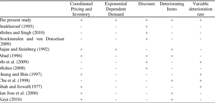
addition, (Aggarwal 1978) reviewed and modified the model proposed by (Shah and Jaiswal 1977). Elion and Malaya (1970) were the first to review the pricing of perishable goods. They assumed that goods had a useful life and their deterioration did not occur before the expiration date. Moreover, (Shane 1996) developed the pricing and inventory control of perishable goods by considering delays in payments and the issue of discounts in transportation. (San José, Sicilia et al. 2006) examined the pricing and inventory control of perishable goods such that a downward demand would be a two-criterion function. Furthermore, (Skouri and Papachristos 2003) considered the pricing and inventory control in a time-dependent rate of demand and corruption. (Hwang and Shinn 1997) solved the pricing and inventory control of perishable goods by considering the exponential deterioration. (Su, Xiao et al. 1999) re-solved the models proposed by (Hwang and Shinn 1997) while considering fixed demand. Later, (Chang, Hung et al. 2002) studied the inventory and pricing model for perishable goods, taking into account linear price dependency and delays in payments. (Mishra and Mishra 2008) investigated the pricing of goods for the inventory model of perishable goods. (He, Prasad et al. 2007) focused on the problem of determining the optimal inventory policy for the EOQ of perishable goods in the case of multiple markets. Moreover, (Chang, Hung et al. 2002) determined inventory policy for perishable goods, taking into account the VMI inventory management model. (Avinadav, Herbon et al. 2013) also examined the problem of inventory and pricing policy for obsolete goods in a state that demand function was considered simultaneously dependent on time and price. An interesting point in this article was that the three-variable objective function of the paper had become a function of one variable using mathematical methods, and, accordingly, the quasi-convexity of the objective function was proven. (He, Prasad et al. 2007) examined the policy of re-filling and pricing by taking into account the price-dependent demand which declines over time. Moreover, (Mo, Mi et al. 2009) studied the inventory and pricing model in terms of demand dependence on price and inventory levels. Also, (Hsieh, Dye et al. 2010) investigated a problem similar to that examined by (Mo, Mi et al. 2009), with the difference that the demand function gradually decreased, ultimately reaching zero. Furthermore, (Teng, Ouyang et al. 2007) Studied the pricing and size of the economic order problem for deteriorating products. Assumptions such as a constant rate of deterioration and price of time-dependent maintenance were considered in that study. The researchers presented a comparison against the model developed by (Abad 2003) in terms of profit per unit time. (Urban 1995) developed the model presented by (Alfares 2007) by releasing the assumption that the inventory becomes zero at the end of the re-processing period. In fact, he considered the possibility of positive stock at the end of each period. Thus, for each product, the remainder of the product at the end of each period of the sales price was less than the sales price during the sales period. Wu proposed a challenge for dairy products in 2018, which resulted in reduced wastes from dairy products(Wu, Lu et al. 2018). In 2019, Rohmer evaluated the supply chain in chain stores(Rohmer, Claassen et al. 2019). In recent years, a definitive inventory model has been proposed for corrosive commodities with a price-dependent demand, in which the demand rate and the rate of deterioration of continuous and differentiable functions are based on price and time, respectively. liu consider a new decision issue for perishable products in production inventory with pricing and promotion for a single-vendor multi-buyer system comprising one manufacturer and multiple retailers. First, a centralized decision model with a vendor managed inventory (VMI) control system under a just-in-time shipment policy is developed (Liu, Zhang et al. 2018). Table 1 presents a summary of selected articles on the inventory control and pricing of perishable products that are most relevant to the present research.
123
Table 1. Summary of selected papers Coordinated
Pricing and Inventory
Exponential Dependent
Demand
Discount Deteriorating Items
Variable deterioration
rate
The present study + + + + +
Benkherouf (1995) - - + - -
Mishra and Singh (2010) - - + - -
Brockmeulen and ven Donselaar (2009)
- - + - -
Rajan and Steinberg (1992) + + - + -
Abad (1996) + - + + -
Mo et al. (2009) - - + - +
Mishra (2008) - - + - -
Huang and Shin (1997) + - - - +
Chu et al. (1998) - - - + +
Shah and Jizwall(1977) + - - - +
San Jose et al. (2006) + - - + -
Kaya (2016) + - - + -
The present study aimed to propose and evaluate a model for ways to reduce wastes from dairy products. To this end, a model was developed for determining the optimal price and inventory control for products with a constant rate of deterioration and demand, depending on time and cost with an exponential distribution. The proposed model was utilized due to increasing the seller's profit, increasing sales, reducing the losses caused by spoilage, and giving suitable discounts to buyers. One of the research gaps in the existing literature is the study of degenerate products under uncertain time. While researchers and managers have paid considerable attention to the development and use of inventory models for decaying products, But in most developed models, time is assumed to be a parameter with a constant interval. In this research, by providing a model before the product reaches the expiration date over different time periods, the discount is considered, so that the inventory end of the period is zero. By using the discount, creates a craving for the customer and sells more products. One of the features of this model is to consider the rate of corruption as constant. Scientists like Kaya have taken the demand in a linear function, In this study, looking at demand has made it closer to the real world. Considering the non-linear maintenance cost for modeling inventory models for degradable products, especially corrosive products (products with a certain lifecycle), it is interesting to note that its applicability has been shown in various ways. In this study, using the nonlinear maintenance cost of the model makes it very difficult for us to solve it. For this purpose, the model is described in section 2, and the model’s assumptions and symbols used are explained in section 2-1. Then, the method of developing an inventory model is discussed in section 3, and they way to solve it is expressed in section 4. Section 5 describes the sensitivity analysis of the model, and section 6 provides the conclusions and suggestions for future research.
2-1- Degradation modeling approach in developed models
By studying the developed inventory models in the field of perishable products, the existing research can be classified into three categories according to how the process of product degradation is modeled. This classification is schematically shown in figure. 1.
124
Fig1. Different approaches to modeling degradation
Few articles have been devoted to modeling the product decay process using the decay rate function in the inventory function statement in hand (Category 1 features) as well as non-linear maintenance (Category 2 features). Goyal and Giri (2003) considered the fixed decay rate and maintenance cost as a general function of time, demand depending on sales prices, and minor backward demand to minimize the cost of a production system. In the present study, a mathematical model was presented by taking into account a fixed decay rate and nonlinear maintenance cost. As already mentioned, the goal of the model was to maximize profits. To this end, the total cost was first determined, and the expected profit was obtained by lowering the earnings.
3
-
Notations and assumptions
For convenience, the following notations and assumptions are adopted throughout the entire paper.
3-1- Parameters:
C: Purchasing cost per unit.
h: Holding or carrying cost per unit per unit of time.
m: Maximum life time in units of time. S: Salvage price per unit.
D (t, p): demand rate is denoted by D(t, p) or D. a(t): the age-dependent freshness at time t.
: decay rate of products.
N: the number of different prices used in an inventory cycle.
3-2- Decision variables
T: Replenishment cycle time in units of time. R
: total revenue in an inventory cycle. P: Price per unit
3-3- Assumptions
Perishable products cannot be repaired or replaced during the time period.
Deduction is not allowed.
The stock reaches zero at the end of the period. Category 1
Inventory Function:
) ( ) ( ) ( ) ( ) (
t D t P t I t dt
t
dI
Holding Cost:
htI
H
Degradation modeling approach in developed models
Category 2
Inventory Function:
) ( ) ( ) (
t D t P dt
t
dI
Holding Cost:
Category 3
Inventory Function:
) ( ) ( ) ( ) ( ) (
t D t P t I t dt
t
dI
Holding Cost:
) , (t I Z H
125
The demand rate D is proportional to an exponential function of the price P. Thus, p
i e
m t m t
p
D( , )
θ has a constant rate independent of the other products.
3-4-
Mathematical model
In this study, given the demand for i e p m
t m t
p
D( , )
which has an exponential distribution, in terms of price and time, it is trying to get closer to reality. One of the research gaps in the existing literature is the study of degenerate products under uncertain time. While researchers and managers have paid considerable attention to the development and use of inventory models for decaying products but in most developed models, time is assumed to be a parameter with a constant interval. In this research, by providing a model before the product reaches the expiration date over different time periods, the discount is considered, so that the inventory end of the period is zero. Using the discount, it creates a desire for the customer and sells the product more. One of the features of this model is to consider the rate of corruption as constant. In this chapter, by presenting a mathematical model, we study the optimum time for price changes, optimal prices, optimum order quantity, and also the analysis of the effect of different parameters in the optimal solution.The most prominent feature of this model is: Limited planning horizon
Nonlinear maintenance cost (corrosive products) / single product /
Non-deterministic conditions: probable time-demand has exponential distribution, depending on price and time
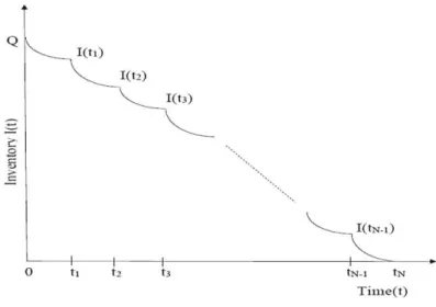
In order to determine the desired parameters, including the price, the amount, and the time of each order, it is necessary to correctly express the behavior of the system under study in terms of mathematical formulas, as shown in figure 2 (Kaya and Polat 2017).
Fig 2. Illustration of inventory process
We describe the inventory function I (t) by the differential equation (1) which consists ofthe decay rate and the price- and time-dependent demand rate, D(p, t), such that:
126 I(t)
D(p (t) , t) I(t)
t
(1)
Since the inventory function changes every time the price is changed, we let Ii(t)denote the inventory function for any timet ∈ [
t
i-1,t
i). We also letI (t
i) denote the inventory level at the end of the time period[
t
i-1,
t
i). Note that the inventory levelIi(t)will be equal to the inventory consumed from time tto ti due tosales anddecayplus I (
t
i) as stated below:i
t
t s t
i i
t
I (t)e
e D(p ,s) dsce (2) From now on, in order to obtain explicit analytical results, we use the exponential demand function that is commonly used in literature (Feng, Chan et al. 2017), and depends on both price and time:p i e m t m t p
D( , )
(3) Using the exponentialdemand function, the inventory equation can be written as:) ( ) (
)
(
)
(
p s t t tt t i i i
e
c
ds
e
e
m
s
m
t
I
(4) Let us solve equation (3) using integration by parts:) ( ) ( 2 ) (
)
1
(
1
1
)
(
)
(
)
(
p i t t p t t t ti
i i
i i
i
e
e
c
e
m
m
t
m
e
m
t
m
e
t
I
(5)
We note that since at the end of the cycle, all the inventory would be consumed (otherwise,it would not be an optimal solution and ordering one less at time zero would yield a better result), i.e.,I (tN) =0, thus by using the above equation and going backwards, one can explicitly find all I(
t
i)values and Ii(t)equations. Similarly, we can find the order level Q = I(
t
0) where t0 = 0 from the above equation.Explicitly, we can write Qand I(
t
i) as follows:
1
1 11
)
1
1
1
1
(
1 t p 2 t tp
e
c
e
e
m
e
m
t
m
e
Q
i
(6)
( )
( ) 2 1 ) ( 1 1 1 11
1
1
1
i i ti ti i ti pi titi ti tiN i p
e
c
e
e
m
e
m
t
m
e
m
t
m
e
Q
(7)
127 ) 8 (
2 1 2 1 2 1 1 i i i i p t t p i t t m t t e dt e m s m s i i i i
Then, we find the revenue in an interval by multiplying the demand by the price in that cycle, and the total revenue in an inventory cycle would be the sum of all the revenues earned at each interval. The total revenue, R, can be determined as follows:
(9)
2
1 2 1 1 2
n p i i p i i ii i
R p t t
m e t t e p i i
We also calculate the inventory cost, H, in the system by calculating the area under the inventory curve
shown in figure 2.
( )
1 2 ) ( 3 2 1 2 1 ) ( 1 1 1 1 1 11
1
1
1
1
)
1
(
1
)
(
2
1
1
1
)
(
i i i i i i i i i i i i i t t i i p t t p i i p i i p t t i p n i n i t t i He
c
t
t
e
m
e
e
m
t
t
m
e
t
t
e
e
m
t
m
e
h
dt
t
I
h
Finally, the profit per unit time function is obtained by taking the difference between total revenue and total cost during an inventory cycle and dividing that value by the length of an inventory cycle. As a result, we can write our problem as follows:
N i t t i i p t t p i i p i i p t t i p i i i p i i p i N N C CQ A e c t t e m e e m t t m e t t e e m t m e h t t p m e t t e p TN MAX i i i i i i i i i i i i i 1 ) ( 1 2 ) ( 3 2 1 2 1 ) ( 2 1 2 1 ) ( )) ( ( 1 1 1 1 1 ) 1 ( 1 ) ( 2 1 1 1 2 1 1 1 1
(10)128
St:
1
,
2
,....
0
,...,
1
0
,...,
1
0
,...,
1
0
0 1
N
t
N
i
p
N
i
t
t
N
i
e
m
t
m
i i i p
p p3 e ip (2it t) 2 i
p p e (2it t)
1 [[3 2e it 3e ip t 1 i 3
i
3 2 2 mt 2 mt
mt p
p p 3 p p
3 e i( it mt)(1 e t) 3 e it 1 e ip (2iti t) 3 e i 3 e i
h ]
2 2 mt mt 2
mt m
p p
3 e i( it mt)e t 3 e i(e t 1) p p t
(i t) 3 4
i i
c[ ]][2e c 2e c ] r e c
2 mt mt
pi t 2 2 pi 3 4 (i t) 3 4 (i 1) 2
2e c t r e c 2r e cmi t e cmi
(i 1) (i 1) (i 1) (i 1)
3 4 2 3 4 3 4 3 3 4 3
3t e ci 3t e ci t e cm t e hm t e ct
p
pi 2 3 2 i t 3 3 pi t 3 2 pi t
2e h t e ah m t e aci t e ahi
p t 1 1 p p p t
3 3 i 2 2 i 2 2 i 2 2 i 2 2
t e ac m] [ (2 e r i 2 e p mri 2e ci r
2 4 4 4 m t
pi t 2 2 pi 2 pi 2 2 pi t 2
2e c mr 2e h mr e p ri 2e hi r
pi t 2 pi 2 2 pi 2 2 pi 2 pi 2 2
2e h mr 4e r 4e mr 2e h 2e r 6
2e
pi t pi t pi t 2
ct 2e c 2e c] 0
t 3(2i 1) h(m i)(1 e ) t
p ti 0
2 2m 2m
(11) At the end, the optimal sales price is obtained by taking into account the limitations with this equation(11).
2 2 ( 2)
2 1 2 1 1 2 2 ) 1 2 ( 2 2 mt e c m e i m c m h mt h m i h t h m e i m h m i t i t m m p t t t i
129
3-5-
Proof of the convexity of the
objective function
One common and traditional approach to proving the convexity of a function that is twice-differentiable by decision variables is to form a Hessian matrix and prove that the matrix is positive. Many researchers such as (Goh 1994) and (Chen and Chang 2010) have used this approach to solve inventory models.
t
z
t
p
z
t
p
z
p
z
2 2 2
2 2
2
(12)
The number of decision variables in the objective function is limited to two and, therefore the dimensions of the Hessian matrix are 2*2. However, due to various parameters, relative complexity, and the relatively long form of target function, we cannot directly utilize this approach. In order to find the optimal solution, in the first step, the goal function has to be proved, and in the next step, optimal solutions are obtained using the proposed algorithm. This matrix actually represents the degree of local curvature of the function in question for its variables. In this study, to derive convexity, derivatives derived from the Hessian matrix are placed in the problem limits and only if convexity conditions are satisfied.
4- Genetic algorithm
The genetic algorithm is a programming technique that employs genetic evolution as a problem-solving model. The problem which needs to be solved has some inputs that are converted into solutions from the genetic evolution by the genetically engineered benchmarked process. Then, the solutions are evaluated as candidates by the fitness function and, if the exit condition of the problem is provided, the algorithm ends. Generally, an algorithm is based on repetition and most of its processes are selected at random, composed of the fitting, display, selection, and change functions.The genetic algorithm is an optimization method based on naturally inspired genetic operations. It uses selection, mutation, and crossover operations to achieve its optimization goal. A chromosome in our model is an array with N values where the element at i denotes the value of
t
i.Since N is a decision variable, the algorithm was applied for different N values, and the optimal N was obtained through enumeration. We then applied crossover operations to generate new populations using one-point variable-length crossovers. Next, we formed a mating pool with the offspring and the original population. Then, by generating random numbers, chromosomes with higher fitness values were selected in the next generation. Afterwards, we took two parents, cut them at a random position, and then swapped them. For each chromosome pair, the probability of crossover was random. Therefore, during each iteration, 15 pairs were created and crossover was applied if the default crossover probability was less than the random number generated by the code as the crossover probability. The pseudo-code for our algorithm is as follows:Pseudo-Code for the Genetic Algorithm
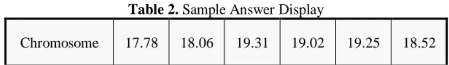
Step 1: The given answer is represented as a matrix with one row and N columns, and its elements are in the form of continuous numbers between 0 and a predetermined upper limit for variable
t
i. An example of this matrix for N=6 is presented in table 2.Table 2. Sample Answer Display
18.52 19.25
19.02 19.31
18.06 17.78
Chromosome
Based on the above matrix, variable
t
i is calculated as described in the evaluation function section.Step 2: The evaluation function is the only criterion for guiding the genetic algorithm while searching to find an appropriate response. In this research, the objective function of the problem is the
130
algorithm evaluation function. First, we need to make some corrections to the display of the result so that we can calculate the variables and also calculate the amount of the target function. Because the proposed model has a limit
t
i
t
i1
, to satisfy this limitation, it suffices to arrange the generated matrix in the display section of the answer from small to large.Step 3: Selection of chromosomes from the current population is also performed in a variety of ways. We
have used the selection of roulette wheels in this research. The general principles of selection in this method are that, in the first step, for each chromosome of the present population, we assign the probability that shows the chances of selecting that chromosome for transmission to the intersection. In the second step, using a method and according to the probability of the chromosomes, we select some of them for transfer to the intersection. Keep in mind that probabilities are assigned to chromosomes in a distributed form. In other words, the total probability for all chromosomes should be equal to 1.
Step 4: The latter side of Darwin's theory states that, after the production of the offspring’s chromosomes,
random mutations may occur in some of the produced chromosomes, resulting in better or worse chromosomal optimization. We also use this property of genetic algorithms and create mutations in the answers generated for the problem. This method is implemented in different ways depending on the algorithm designer's innovation.
Step 5: In this research, the criterion for maximum generation was employed as a stopping criterion. Using this rule, the genetic algorithm stops after a certain number of generations.
4-1- Setting the Parameter of the Genetic Algorithm
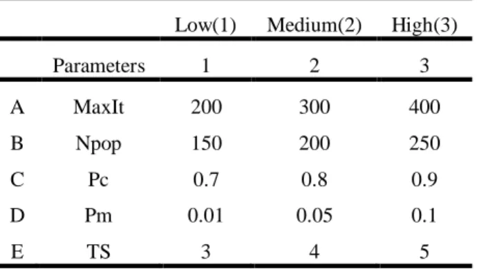
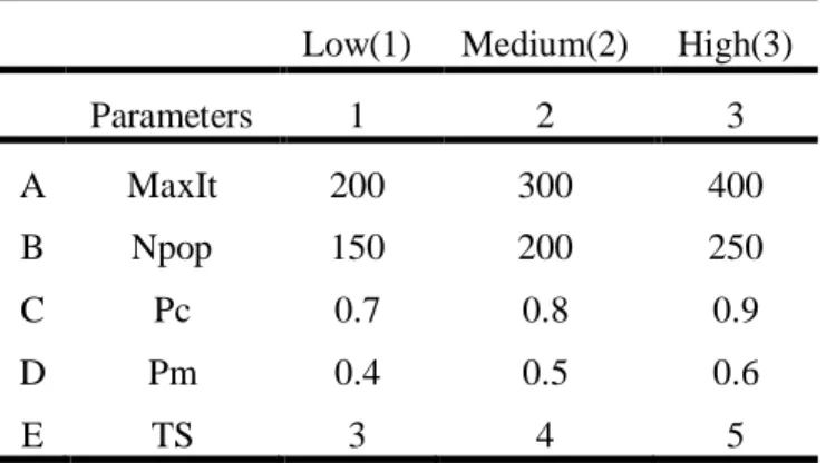
To control the parameters of the proposed genetic algorithm, the Taguchi method, from the Minitab software, was used. The effective parameters of the genetic algorithm were the maximum number of repetitions, intersection rate, mutation rate, and population. For each of these factors, three levels were defined as follows:
Table 3. Parameters and levels for setting the parameter of the genetic algorithm Low(1) Medium(2) High(3)
Parameters 1 2 3
A MaxIt 200 300 400
B Npop 150 200 250
C Pc 0.7 0.8 0.9
D Pm 0.01 0.05 0.1
E TS 3 4 5
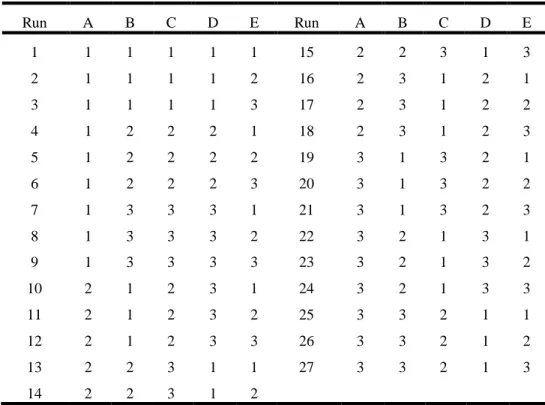
The number of tests required for 5 factors and 3 levels was 27. The tests for the parameters of the genetic algorithm were as follows:
131
Table 4. Tests designed to adjust the parameter by Taguchi method
Run A B C D E Run A B C D E
1 1 1 1 1 1 15 2 2 3 1 3
2 1 1 1 1 2 16 2 3 1 2 1
3 1 1 1 1 3 17 2 3 1 2 2
4 1 2 2 2 1 18 2 3 1 2 3
5 1 2 2 2 2 19 3 1 3 2 1
6 1 2 2 2 3 20 3 1 3 2 2
7 1 3 3 3 1 21 3 1 3 2 3
8 1 3 3 3 2 22 3 2 1 3 1
9 1 3 3 3 3 23 3 2 1 3 2
10 2 1 2 3 1 24 3 2 1 3 3
11 2 1 2 3 2 25 3 3 2 1 1
12 2 1 2 3 3 26 3 3 2 1 2
13 2 2 3 1 1 27 3 3 2 1 3
14 2 2 3 1 2
After performing the experiments for a specific problem using the presented genetic algorithm, the following results were obtained:
Table 5. Results of experiments designed to set the parameters of the genetic algorithm by Taguchi method Run Obj. Fun Run Obj. Fun Run Obj. Fun
1 -185.2 11 -0.6 21 -116.4
2 -160.1 12 -24.4 22 12.4
3 -109.4 13 -84.7 23 78.9
4 -61.5 14 -6.8 24 -26.3
5 -23.1 15 -163.4 25 -38.7
6 -81.7 16 -4.1 26 -83.3
7 -15.5 17 -97.4 27 81.3
8 0.2 18 -48.0
9 12.8 19 -73.8
10 -20.2 20 32.3
It is noteworthy that the results obtained from the experiments must be converted to the same dimensions. A method for this conversion is the RPD method.
132
RPD=| Method sol - Best Sol |*100/ |Best Sol |
In the above statement, Method Sol is the amount of the results obtained from the implementation of the algorithm, and Best Sol is the best answer obtained from 27 experiments. After the above conversion, the results of tests were modified according to the following table:
Table 6. Normalized results for adjusting the parameter of the genetic algorithm by Taguchi method Run Obj. Fun Run Obj. Fun Run Obj. Fun
1 327.87 11 100.77 21 243.16
2 297.00 12 129.98 22 84.72
3 234.62 13 204.16 23 2.88
4 175.62 14 108.36 24 132.31
5 128.37 15 301.02 25 147.67
6 200.55 16 105.05 26 202.48
7 119.07 17 219.89 27 0.00
8 99.72 18 159.02
9 84.26 19 190.74
10 124.87 20 60.30
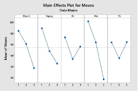
After analysis using the Taguchi method in Minitab for the genetic algorithm, the following results were obtained:
Fig 3.Results from Minitab Software for Genetic Algorithms
The general rule about the shape of the graph is that, whenever the value of the vertical axis is greater, the value of the objective function is better and, therefore, we can introduce the parameter level with the highest value as the selective parameter. For example, for a population, we can choose a population of 250 as a selective parameter. After performing the analysis and based on the tests for the genetic algorithm, the optimal levels for the parameters of maximum repetition of the algorithm, initial
133
population, intersection rate, mutation rate, and racing choice algorithm were 1, 3, 1, 2, and 2, respectively.
Table 7. Results from Minitab Software for Genetic Algorithms
Low(1) Medium(2) High(3)
Parameters 1 2 3
A MaxIt 200 300 400
B Npop 150 200 250
C Pc 0.7 0.8 0.9
D Pm 0.4 0.5 0.6
E TS 3 4 5
5- Computational studies
In this section, the issue of pricing and inventory control was analyzed using the 950 g yogurt product produced by Kaleh factory (Iran) over a given time period. The related data used was maximum number of potential consumers α = 200, the price efficiency of demand λ = 0.1, c=$20/unit, h=$5/unit/year, m=0.06 years, the decay rate of products θ=0.05, and thefixed order cost A=5000.
In addition, when Nprices are used in an inventory cycle, it means that N - 1 price changes are made; thus we use a linear cost function C(N) = (N - 1) f for changing prices. The proposed algorithm was applied to obtain the optimal solution for the case study.
033
.
12
TN
,
1186 . 45
*
Q
To evaluate the behavior of the proposed model proportional to its parameters, the sensitivity analysis of various parameters and functions was performed. The sensitivity analysis was conducted such that each parameter in every execution remained constant except for one parameter, which underwent enough changes of different magnitudes
.
134
Table 8.Sensitivity analysis
TN Price
Order Size Profit
12.0339 35.1498
33.7475 32.2343 30.8079 29.3415 45.1186
173.267
200
12.079 35.1307
33.723 32.3159 30.8768 29.418 48.8686
135.0615
250
12.0936 35.1572
33.7378 32.323 30.8628 29.3382 51.6387
141.9801
4 c
19.931 38.1434
36.5144 34.8514 33.1784 31.2488 30.6192
1769.5528
6
c
19.9904 28.7602
27.8768 27.0064 26.1155 25.1971 51.8343
148.2361
= 0. 6
12.7977 34.2411
32.521 30.7833 29.0323 27.2877 24.4563
409.4848
= 0.212.5455 29.4296
28.2841 27.1339 25.9581 24.7605 27.9599
538.2133
2
.
0
H
19.9974 29.0617
28.2498 27.421 26.4764 25.5914 35.0105
819.6388
05 . 0
H
12.6662 29.1906
28.2649 27.3271 26.3595 25.3388 35.566
721.526
6000 A
12.7708 29.1905
28.2534 27.3183 26.3227 25.3311 31.843
957.6063
4000 A
135
The results of sensitivity analysis indicated that, when the deterioration rate increases, the time rate decreases and the sales price increases. Also, reducing the rate of deterioration should be put on the retailer's agenda. The results demonstrated that, by increasing the deterioration rate by 2%, the purchase cost increases by 5%, implying that the manufacturer would increase his/her sales price to reduce the effect of deterioration, which would further increase his/her profit. Nevertheless, this approach does not seem very rational because the increase in the producer's price may result a reduction in the retailer’s order and, as a result, have a negative effect on the producer's profit. Therefore, similar to the retailer, the manufacturer should seek to reduce deterioration in the system. If the rate of decay
increases by 2%, then the period of time decreases, and the sales price increases by 3%. When the value of C increases, the sales price also increases. An increase of 2000 in the amount of startup cost A would lead to a 6% decrease in the profit value of the target function and the sales price of the producer. By keeping
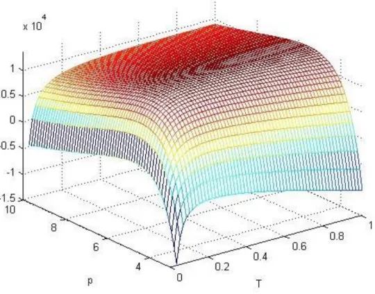
and λ constant, when t increases, the amount of economic order and total system profits will increase and the optimal sales price will decrease. By increasing the value of the deterioration rate and keeping the other parameters constant, the amount of economic order, total profit of the system, and optimal price increases. Based on the analysis made, managers can consider marketing measures such as product discounts by examining the expiry date of perishable products. Also, managers can increase product sales by using a number of breakpoints or periods of discounts. Managers can control inventory by controlling the maintenance cost, purchase cost, and the order amount. In this study, by analyzing the sensitivity of important parameters, we determine the relationship between the parameters and, in view of the demand, bridge the gap between the model and the real world.Fig 4. Profit function display
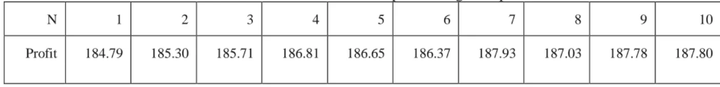
5-1- Effect of the number of price changes on profit
In the present study, sales could be increased by increasing the number of discount points. In addition, the number of discount points, the optimal sales price, and the total profit of the system decrease with an increase in the price elasticity index. The reason is that, with an increase in the amount of alpha, there is a decrease in demand which, in turn, leads to a decrease in the amount of economic order, followed by a
136
decrease in system profits. Using the model presented in this research, decision makers in different areas of perishable product marketing can determine the number of breakpoints and or price levels for their products in a way that maximizes their profits. For example, in the numerical example presented, the number of proposed points comprised five price levels
.
Table 10. Effect of the number of price changes on profit
10 9
8 7
6 5
4 3
2 1
N
187.80 187.78
187.03 187.93
186.37 186.65
186.81 185.71
185.30 184.79
Profit
6- Conclusion and future research
Inventory control and pricing are known as two pillars of supply chain management. That is why, in recent years, pricing and inventory control issues in the supply chain management of perishable products has attracted much more attention than before. In the present research, by developing a mathematical model to price and control the inventory of perishable products, optimal-order quantities and points of price changes were determined. For the first time, the demand distribution for perishable products was considered exponentially. Also, to satisfy the condition of decreasing the price chart over time, the convexity of the objective function was added to the model as a constraint. Due to the complexity of the problem, the method used in this study was the genetic algorithm. By analyzing the effect of different parameters and the optimal solution, the results showed that, by increasing the decay rate by 2%, the amount of purchase cost increases by 5%, implying that the manufacturer will increase their sales price to reduce the effect of deterioration, thereby increasing profit. However, this approach does not seem to be a logical behavior because increasing the price may result in a reduction in the retailer’s ordered quantity, and, as a result, have a negative effect on the producer's profit. Therefore, similar to the retailer, the manufacturer should seek to reduce the decay rate of perishable goods in the system. When decay rate
increases by 2%, the time period shortens, and the sales price increases by 3%. Moreover, the sales price increases when the value of per unit cost C increases.
Finally, the results and findings of this study are: By maintaining the problem variables and increasing the maintenance cost (h), the optimal reappraisal period, the total profits of the inventory system increase. These results indicate that when the cost of maintaining a unit of goods increases, the retailer prefers to order a lower amount of goods and maintain that amount of goods for a shorter time. This indicates the decrease in the amount of economic order, which results from the model also reflects on this issue.
By keeping the problem variables constant, when t increases, The amount of economic order
*w
Q and total profit of the system increase and the optimal sales price decreases.
With the increase in the value of the deterioration rate and the remaining parameters remaining, the amount of economic order, the total profit of the system and the optimal sales price increase. The number of discount points, The optimal sales price and overall system profits are reduced by increasing the price elasticity index. The reason is that with increasing the amount of alpha, there is a decrease in demand. The decline in demand results in a reduction in the amount of economic order, followed by a decrease in the system profits.
Based on the results obtained and the study of previous research, the following suggestions can be made for future research:
The application of fuzzy concepts and the demand function in general for improvement in the mathematical model
137
The combination of closed-loop supply chain and corrupt products that, After expiration they have the ability to turn into other products, such as turning fruits into fruit juice.
By applying five levels, retailers, manufacturers, customers, recycling, distributor to develop the model and solve it publicly (all products). As shown in the results of numerical examples, decay rates have a high impact on all optimization parameters. By investing in maintenance technologies, the decay rate can be controlled, so considering the amount of investment in path maintenance technologies will be for future studies.
Considering the periods when they follow the statistical functions, followed by the development of the model by addressing the cost of space, the cost of the shortage, and the introduction of a locational discussion.
References
Abad, P. L. (2003). "Optimal pricing and lot-sizing under conditions of perishability, finite production and partial backordering and lost sale." European Journal of Operational Research 144(3): 677-685. Aggarwal, S. (1978). "A note on an order-level inventory model for a system with constant rate of deterioration." Opsearch 15(4): 184-187.
Alfares, H. K. (2007). "Inventory model with stock-level dependent demand rate and variable holding cost." International Journal of Production Economics 108(1-2): 259-265.
Avinadav, T., A. Herbon and U. Spiegel (2013). "Optimal inventory policy for a perishable item with demand function sensitive to price and time." International Journal of Production Economics 144(2): 497-506.
Bahari-Kashani, H. (1989). "Replenishment schedule for deteriorating items with time-proportional demand." Journal of the operational research society 40(1): 75-81.
Broekmeulen, R. A. and K. H. Van Donselaar (2009). "A heuristic to manage perishable inventory with batch ordering, positive lead-times, and time-varying demand." Computers & Operations Research
36(11): 3013-3018.
Cave, E. F. (1963). "The Past and Present of Trauma." Surgical Clinics of North America 43(2): 317-327. Chang, H.-J., C.-H. Hung and C.-Y. Dye (2002). "A finite time horizon inventory model with deterioration and time-value of money under the conditions of permissible delay in payments." International Journal of Systems Science 33(2): 141-151.
Chen, T.-H. and H.-M. Chang (2010). "Optimal ordering and pricing policies for deteriorating items in one-vendor multi-retailer supply chain." The International Journal of Advanced Manufacturing Technology 49(1-4): 341-355.
CHUNG, K.-J. and P.-S. TING (1994). "On replenishment schedule for deteriorating items with time-proportional demand." Production Planning & Control 5(4): 392-396.
Covert, R. P. and G. C. Philip (1973). "An EOQ model for items with Weibull distribution deterioration." AIIE transactions 5(4): 323-326.
138
Donaldson, W. (1977). "Inventory replenishment policy for a linear trend in demand—an analytical solution." Journal of the operational research society 28(3): 663-670.
Feng, L., Y.-L. Chan and L. E. Cárdenas-Barrón (2017). "Pricing and lot-sizing polices for perishable goods when the demand depends on selling price, displayed stocks, and expiration date." International Journal of Production Economics 185: 11-20.
Ghare, P. (1963). "A model for an exponentially decaying inventory." J. ind. Engng 14: 238-243.
Goh, M. (1994). "EOQ models with general demand and holding cost functions." European Journal of Operational Research 73(1): 50-54.
Goswami, A. and K. Chaudhuri (1992). "Variations of order-level inventory models for deteriorating items." International Journal of Production Economics 27(2): 111-117.
Goyal, S. and B. C. Giri (2003). "The production–inventory problem of a product with time varying demand, production and deterioration rates." European Journal of Operational Research 147(3): 549-557. He, X., A. Prasad, S. P. Sethi and G. J. Gutierrez (2007). "A survey of Stackelberg differential game models in supply and marketing channels." Journal of Systems Science and Systems Engineering 16(4): 385-413.
Hsieh, T.-P., C.-Y. Dye and L.-Y. Ouyang (2010). "Optimal lot size for an item with partial backlogging rate when demand is stimulated by inventory above a certain stock level." Mathematical and Computer Modelling 51(1-2): 13-32.
Hwang, H. and S. W. Shinn (1997). "Retailer's pricing and lot sizing policy for exponentially deteriorating products under the condition of permissible delay in payments." Computers & Operations Research 24(6): 539-547.
Kaya, O. and A. L. Polat (2017). "Coordinated pricing and inventory decisions for perishable products." OR spectrum 39(2): 589-606.
Lee, Y.-P. and C.-Y. Dye (2012). "An inventory model for deteriorating items under stock-dependent demand and controllable deterioration rate." Computers & Industrial Engineering 63(2): 474-482. Liu, H., J. Zhang, C. Zhou and Y. Ru (2018). "Optimal purchase and inventory retrieval policies for perishable seasonal agricultural products." Omega 79: 133-145.
Mishra, S. S. and P. Mishra (2008). "Price determination for an EOQ model for deteriorating items under perfect competition." Computers & Mathematics with Applications 56(4): 1082-1101.
Mo, J., F. Mi, F. Zhou and H. Pan (2009). "A note on an EOQ model with stock and price sensitive demand." Mathematical and Computer Modelling 49(9-10): 2029-2036.
Rohmer, S., G. Claassen and G. Laporte (2019). "A Two-Echelon Inventory-Routing Problem for Perishable Products." Computers & Operations Research.
Rao, W. S., S. Goyal and G. Venkataraman (1963). "Effect of inoculation of Aulosira fertilissima on rice plants." Current Science 32(8): 366-367.
139
San José, L., J. Sicilia and J. García-Laguna (2006). "Analysis of an inventory system with exponential partial backordering." International Journal of Production Economics 100(1): 76-86.
Shah, Y. and M. Jaiswal (1977). "An order-level inventory model for a system with constant rate of deterioration." Opsearch 14(3): 174-184.
Shane, S. A. (1996). "Hybrid organizational arrangements and their implications for firm growth and survival: A study of new franchisors." Academy of management journal 39(1): 216-234.
Skouri, K. and S. Papachristos (2003). "Optimal stopping and restarting production times for an EOQ model with deteriorating items and time-dependent partial backlogging." International Journal of Production Economics 81: 525-531.
Su, B., J. Xiao, P. Underhill, R. Deka, W. Zhang, J. Akey, W. Huang, D. Shen, D. Lu and J. Luo (1999). "Y- Chromosome evidence for a northward migration of modern humans into Eastern Asia during the last Ice Age." The American Journal of Human Genetics 65(6): 1718-1724.
Teng, J.-T., L.-Y. Ouyang and L.-H. Chen (2007). "A comparison between two pricing and lot-sizing models with partial backlogging and deteriorated items." International Journal of Production Economics
105(1): 190-203.
Urban, T. L. (1995). "Inventory models with the demand rate dependent on stock and shortage levels." International Journal of Production Economics 40(1): 21-28.
Wu, X., Y. Lu, H. Xu, M. Lv, D. Hu, Z. He, L. Liu, Z. Wang and Y. Feng (2018). "Challenges to improve the safety of dairy products in China." Trends in food science & technology 76: 6-14.