Vol 3, No 12 (2012)

Available online throug

ISSN 2229 – 5046

APPLICATION OF THE MULTIGRID TECHNIQUE FOR THE NUMERICAL

SOLUTION OF THE NON-LINEAR DISPERSIVE WAVES EQUATIONS

Y. M. Abo Essa

(1*)

, T. S. Amer

(2)

and

Ibrahim B.

Abdul

-

Moniem

(3)

Mathematics Department, Faculty of Education and Science (AL-Khurmah Branch),

Taif University, Kingdom of Saudi Arabia.

(1)

Mathematics Department, Faculty of Science, Al-Azhar University, Nasr City 11884, Cairo, Egypt

(2)

Mathematics Department, Faculty of Science, Tanta University, Tanta 31527, Egypt

(Received on: 17-11-12; Revised & Accepted on: 24-12-12)

ABSTRACT

T

he scope of this paper is to obtain the numerical solutions of the Korteweg-de Vries (KdV) equation and the related partial differential equations (namely: the modified Korteweg-de Vries equation (MKdV) and the Korteweg-de Vries-Burgers' equation (KdVB)) using the multigrid method. The difference equation of the Korteweg-de Vries (KdV) equation and the related partial differential equations using the finite difference method are obtained. The computer cods are used to obtain the numerical solutions that compared with the analytical ones to get the

L

₂-errors. The obtained results are compared with another method using

L

₂-errors to show the deviation between them.

Keywords and phrases: multigrid method, wave equation, numerical simulation.

1. INTRODUCTION

The numerical solution of partial differential equations requires some discretization of the domain into a collection of points. A large system of equations comes out from discretization of the same partial differential equations and the optimal method for solving these problems is multigrid method, see [1- 8].

In the past two decades, a great deal of research work has been published on the development of numerical solution of non-linear waves. Various numerical methods are known in order to obtain approximate solutions of the KdV equation, namely: Zabusky and Kruskal method [9], Hopscotch method (Greig and Morris [10]), Galerkin method (Alexander and Morris [11]), Petrove-Galerkin method (Sanz-Serna and Christie [12]), Central finite-difference scheme (Schoombie [13] and Shamardan [14]) and Split step Fourier method (Chan and Kerkhoven [15]).

In this work, we present the numerical solution of three types of non-linear wave equations; namely:

1) The Korteweg-de Vries (KdV) equation of the form

],

,

0

[

],

,

0

[

,

0

,

0

x

X

t

T

u

u

u

u

_t

+

_x

+

ε

_xxx

=

ε

>

∈

∈

(1)

with the initial condition

),

(

)

0

,

(

x

f

x

u

=

(2)

and boundary conditions

.

0

)

,

(

)

,

0

(

,

0

)

,

(

)

,

0

(

=

=

=

=

t

X

u

t

u

t

X

u

t

u

x x

(3)

2) The modified Korteweg-de Vries (MKdV) equation of the form

],

,

0

[

],

,

0

[

,

1

,

0

,

0

)

1

(

p

u

u

u

p

x

X

t

T

u

_t

+

+

p _x

+

ε

_xxx

=

ε

>

≥

∈

∈

(4)

with the initial condition (2) and following the periodicity condition

),

,

(

)

,

(

x

t

u

x

X

t

u

=

+

₍₅₎

3) The Korteweg-de Vries-Burgers' (KdVB) equation of the form

],

,

0

[

],

,

0

[

,

0

,

,

0

x

X

t

T

u

u

u

u

u

_t

+

_x

−

ν

_xx

+

ε

_xxx

=

ν

ε

>

∈

∈

(6)

with the same initial and boundary conditions (2) and (3). Equation (6) was derived by Su and Gradner [16] for a wide class of non-linear systems in the weak non-linearity and long wavelength approximation. In [17] the steady state solution of the KdVB equation has been shown to model plasma shocks propagating perpendicularly to a magnetic field. When diffusion dominates dispersion, the steady state solution of the KdVB equation are monotonic shocks, and when dispersion dominates, the shocks are oscillatory. The KdVB equation has been obtained when including electron inertia effects in the description of weak non-linear plasma waves [18]. The KdVB equation has also been used in a study of wave propagation through liquid field elastic tubes by Johnson [19] and for a description of shallow water waves on viscous fluid by Johnson [20]. Canosa and Gazdag [21], discussed the evolution of non-analytic initial data into a monotonic shock and given brief details of a numerical solution for the KdVB equation using the accurate space derivative method.

In this article, the multigrid technique is developed to solve the initial value problems. Then we can use this technique to find the numerical solutions of Korteweg-de Vries (KdV) equation and its related partial differential equations.

2. NUMERICAL METHOD

The goal of this section is to apply the multigrid method for initial boundary value problem, except that, the upper boundary conditions change with time, in which the initial condition is

u

(

x

,

0

)

=

f

(

x

)

for

0

<

t

<

T

. Dividing the interval of time to

K

parts, we obtain the solutions of the partial differential equation at time

t

₁ and use these solutions as initial values for the next level

u

(

x

,

0

)

=

u

(

x

,

t

1

)

, and for the other, we obtain the solutions at time

T

.

The numbers of points in a coarse grid for this domain are two points.

The class of equations we are dealing within this section are related to the known KdV equation (the types given in (1), (4) and (6)). In all applications we assume a partition

δ

=

{

x

₀

=

0

,

∆

x

,

2

∆

x

,

...,

X

}

for closed interval

[

0

,

X

]

, and

∆

t

mesh in

t

,

∆

x

mesh in

x

.

Let us denote the finite-difference solution

u

(

x

_i

,

t

_n

)

by

u

_i,n. The finite-difference for partial derivatives can be represented as:

).

(

,

)

(

)

(

2

2

2

,

)

(

)

(

2

,

)

(

2

1 , , ,

4 3

, 2 , 1 ,

1 ,

2 ,

2 2

, 1 , , 1 ,

2 ,

1 , 1 ,

t

O

t

u

u

u

x

O

x

u

u

u

u

u

x

O

x

u

u

u

u

x

O

x

u

u

u

n i n i n i t

n i n i n i n i n i xxx

n i n i n i n i xx

n i n i n i x

∆

+

∆

−

=

∆

+

∆

−

+

−

=

∆

+

∆

+

−

=

∆

+

∆

−

=

−

− − +

+

− +

− +

(7)

These derivatives can be used in each equation as needed.

Consider the KdV equation (1) with the initial and the boundary conditions (2) and (3) respectively. We start handling the non-linear term

u

u

_x by expressing in the form

x

u

∂

∂

2

2

1

_{and using central difference}

),

)

(

)

((

4

1

)

(

_{x i,n}

u

_i1,n 2

u

_i1,n 2

x

u

u

₊

−

₋

∆

≈

with an initial sub partition

x

t

,

u

u

_x

2

,

2

∆

∆

, , 1 2 2

1, 1, 3 2, 1, 1, 2,

1

((

)

(

) )

(

2

2

)

0 ;

4

2(

)

1,..., 2

1,

1,..., 2 ,

1,...,

.

k k

i n i n k k k k k k

i n i n i n i n i n i n

k k

u

u

u

u

u

u

u

u

t

x

x

i

n

k

M

ε

−

+ − + + − −

−

+

−

+

−

+

−

=

∆

∆

∆

=

−

=

=

(8)

We apply the full multigrid algorithm for the KdV equation. Assuming the initial condition

u

(

x

,

0

)

=

f

(

x

)

and the solution

u

(

x

,

t

)

,

a

≤

x

≤

b

,

0

≤

t

≤

T

has the usual partition with a space step size

∆

x

and a time step size

∆

t

(

t

_K+1

=

t

_K

+

∆

t

,

K

=

0

,

1

,

2

,

...

).

Step 1:

K

=

0

,

u

(

x

,

0

)

=

f

(

x

).

Step 2: Starting from

k

=

1

in the coarse grid, we can calculate the approximate value

u

_i,n at two points using equation (8) leading to:

1 1 1 2 1 2 1 1 1 1

, , 1

((

1,

)

(

1,

) )

3

[

2,

2

1,

2

1, 2,

];

1,

1, 2,

4

2(

)

i n i n i n i n i n i n i n i n

t

t

u

u

u

u

u

u

u

u

i

n

x

x

ε

− + − + + − −

∆

∆

=

−

−

−

−

+

−

=

=

∆

∆

(9)

and the right hand side is computed from the initial and boundary conditions.

Step 3: Interpolating the grid functions from the coarse grid to fine grid using linear interpolation

I

_kk+1, where k

k k k

u

I

u

+1

=

+1 (10) which can be written explicitly as:

.

1

2

...,

,

0

,

;

)

(

25

.

0

,

1

2

...,

,

0

,

1

2

...,

,

1

;

)

(

5

.

0

,

2

...,

,

1

,

1

2

...,

,

0

;

)

(

5

.

0

,

2

...,

,

1

,

1

2

...,

,

1

;

1 , 1 1 , , 1 ,

1 1 2 , 1 2

1 , , 1

1 2 , 2

, 1 ,

1 2 , 1 2

, 1 2 , 2

−

=

+

+

+

=

−

=

−

=

+

=

=

−

=

+

=

=

−

=

=

+ + + +

+ + +

+ +

+

+ +

+ +

k k

n i k

n i k

n i k

n i k

n i

k k

k n i k

n i k

n i

k k

k n i k

n i k

n i

k k

k n i k

n i

n

i

u

u

u

u

u

n

i

u

u

u

n

i

u

u

u

n

i

u

u

(11)

Step 4: Doing relaxation sweep on

G

k+1 using the point relaxation

1 1 1 2 1 2 1 1 1 1 1 1

, , 1

((

1,

)

(

1,

) )

3

[

2,

2

1,

2

1, 2,

];

1,..., 2

1,

1,..., 2 .

4

2(

)

k k k k k k k k k k

i n i n i n i n i n i n i n i n

t

t

u

u

u

u

u

u

u

u

i

n

x

x

ε

+ + + + + + + + + +

− + − + + − −

∆

∆

=

−

−

−

−

+

−

=

−

=

∆

∆

(12)

Step 5: Computing the residuals

r

k+1 on

G

k+1and injecting them into

G

k using full weighting restriction

I

_kk+1 to get

k

r

as:

,

1 1

+ +

=

k k k k

r

I

r

1 1 1 1 1 1 1 1 1

, 2 1,2 1 2 1,2 1 2 1,2 1 2 1,2 1 2 ,2 1 2 ,2 1 2 1,2 2 1,2 2 ,2

1

[

2(

) 4

]; ,

1,..., 2

1.

16

k k k k k k k k k k k

i n i n i n i n i n i n i n i n i n i n

r

=

r

+_{− −}

+

r

₋+ ₊

+

r

₊+ ₋

+

r

+_{+ +}

+

r

+ ₋

+

r

+ ₊

+

r

₋+

+

r

₊+

+

r

+

i n

=

−

(13)

Step 6: Computing an approximate solution of error

e

k.

Step 7: Interpolating the solution of error

e

k onto

G

k+1,

,

1

1 k k

k k

e

I

e

+

=

+ (14) and adding it to

u

k+1 which is the approximate value of

u

on the fine grid with

k

=

2

.

By taking this solution on coarse grid and repeating steps 3-7, we obtain the approximate values of

u

on the grid with

3

=

Step 8:

K

=

K

+

1

, go to step 2 (lead to the solution at higher time level as needed).

Consider the MKdV equation (4) with the initial and the boundary conditions (2) and (3) respectively. The difference approximation for this equation using (7) takes the form

.

...,

,

1

,

2

...,

,

1

,

1

2

...,

,

1

;

0

]

2

2

[

)

(

2

)

)

(

)

((

2

1

, 2 , 1 , 1 , 2 3 1 , 1 1 , 1 1 , ,

M

k

n

i

u

u

u

u

x

u

u

x

t

u

u

k k k n i k n i k n i k n i p k n i p k n i k n i k n i

=

=

−

=

=

−

+

−

∆

+

−

∆

+

∆

−

− − + + + − + + −

ε

(15)

Using the same pervious steps 1-8 for MKdV equation, we can write

1 1 1 1 1 1 1 1 1 1

, , 1

((

1,

)

(

1,

)

)

3

[

2,

2

1,

2

1, 2,

];

1,

1, 2,

4

2(

)

p p

i n i n i n i n i n i n i n i n

t

t

u

u

u

u

u

u

u

u

i

n

x

x

ε

+ + − + − + + − −

∆

∆

=

−

−

−

−

+

−

=

=

∆

∆

(16)

and the right hand side can be computed from the initial and boundary conditions. Do relaxation sweep using the non-linear point relaxation

1 1 1 1 1 1 1 1 1 1 1 1

, , 1

((

1,

)

(

1,

)

)

3

[

2,

2

1,

2

1, 2,

];

1,..., 2

1,

1,..., 2 .

4

2(

)

k k k p k p k k k k k k

i n i n i n i n i n i n i n i n

t

t

u

u

u

u

u

u

u

u

i

n

x

x

ε

+ + + + + + + + + + + + − + − + + − −

∆

∆

=

−

−

−

−

+

−

=

−

=

∆

∆

(17)

Consider the KdVB equation (6) with the initial and the boundary conditions (2) and (3) respectively. The difference approximation for this equation using (7) takes the form

.

...,

,

1

,

2

...,

,

1

,

1

2

...,

,

1

;

0

)

2

2

(

)

(

2

)

(

2

)

)

(

)

((

4

1

, 2 , 1 , 1 , 2 3 2 , 1 , , 1 2 , 1 2 , 1 1 , ,

M

k

n

i

u

u

u

u

x

x

u

u

u

u

u

x

t

u

u

k k k n i k n i k n i k n i k n i k n i k n i k n i k n i k n i k n i

=

=

−

=

=

−

+

−

∆

+

∆

+

−

−

−

∆

+

∆

−

− − + + − + − + −

ε

ν

(18)

Applying the same pervious steps 1-8 for KdVB equation, we can write

,

2

,

1

,

1

)];

(

4

)

2

2

(

2

)

)

)

((

)

(

)

(

4

[

]

8

)

(

4

[

1

1 , 1 1 , 1 1 , 2 1 , 1 1 , 1 1 , 2 2 1 , 1 2 1 , 1 3 1 1 , 3 3 1 ,

=

=

+

∆

∆

+

−

+

−

∆

−

−

∆

∆

−

∆

∆

∆

+

∆

=

− + − − + + − + −

n

i

u

u

t

x

u

u

u

u

t

u

u

t

x

u

x

t

x

x

u

n i n i n i n i n i n i n i n i n i n i

ν

ε

ν

(19)

and the right hand side is computed from the initial and boundary conditions. Do relaxation sweep using the non-linear point relaxation

.

2

...,

,

1

,

1

2

...,

,

1

)];

(

4

)

2

2

(

2

)

)

)

((

)

(

)

(

4

[

]

8

)

(

4

[

1

1 1 1 , 1 1 , 1 1 , 2 1 , 1 1 , 1 1 , 2 2 1 , 1 2 1 , 1 3 1 1 , 3 3 1 , + + + − + + + − + − + + + + + − + + + − +

=

−

=

+

∆

∆

+

−

+

−

∆

−

−

∆

∆

−

∆

∆

∆

+

∆

=

k k k n i k n i k n i k n i k n i k n i k n i k n i k n i k n i

n

i

u

u

t

x

u

u

u

u

t

u

u

t

x

u

x

t

x

x

u

ν

ε

ν

(20)

3. STABILITY OF FINITE DIFFERENCE SCHEME

In this section we investigate the stability of the numerical scheme (18) for the KdVB equation in the linearised form. We can rewrite the scheme (18) in the linearised form as

, , 1 1, 1, 1, , 1, 2, 1, 1, 2,

2 3

2

2

2

0,

2

(

)

2

()

i n i n i n i n i n i n i n i n i n i n i n

u

u

u

u

u

u

u

u

u

u

u

c

t

x

ν

x

ε

x

− + − + − + + − −

−

−

−

+

−

+

−

+

−

+

=

which may be put in the form

, , 1 1

(

1, 1,

)

(

1,

2

, 1,

)

(

2,

2

1,

2

1, 2,

) 0,

i n i n i n i n i n i n i n i n i n i n i n

u

−

u

₋

+

r u

₊

−

u

₋

−

s u

₊

−

u

+

u

₋

+

p u

∗ ₊

−

u

₊

+

u

₋

−

u

₋

=

(22) where

.

)

(

2

,

)

(

,

2

2 3

1

x

t

p

x

t

s

x

t

c

r

∆

∆

=

∆

∆

=

∆

∆

=

ν

∗

ε

To study the stability of the difference equation (22) we apply the Von-Neumann analysis. Let

u

_i,n

=

e

at

e

ikmx to get

.

0

)

2

2

(

)

2

(

)

(

) 2 ( ) ( ) ( ) 2 ( ) ( ) ( ) ( ) ( 1 ) (

=

−

+

−

+

+

−

−

−

+

−

∆ − ∆ − ∆ + ∆ + ∗ ∆ − ∆ + ∆ − ∆ + ∆ − x x ik at x x ik at x x ik at x x ik at x x ik at x ik at x x ik at x x ik at x x ik at x ik t t a x ik at m m m m m m m m m m m

e

e

e

e

e

e

e

e

p

e

e

e

e

e

e

s

e

e

e

e

r

e

e

e

e

(23)

Divide by

_e

at

_e

ikmx _{to obtain}

,

0

)

2

2

(

2

)

(

)

(

1

2 2 1

=

−

+

−

+

+

+

−

−

+

−

∆ − ∆ − ∆ ∆ ∗ ∆ − ∆ ∆ − ∆ ∆ − x ik x ik x ik x ik x ik x ik x ik x ik t a m m m m m m m m

e

e

e

e

p

s

e

e

s

e

e

r

e

,

0

)

sin

2

2

(sin

2

2

cos

2

sin

2

1

−

e

−a∆t

+

ir

₁

β

∗

−

s

β

∗

+

s

+

ip

∗

β

∗

−

β

∗

=

(24)

where

β

∗

=

k

_m

∆

x

and the amplification factor is denoted by

.

))

2

/

(

sin

4

(

sin

2

))

2

/

(

sin

4

1

(

1

)

1

(cos

sin

4

)

cos

1

(

2

sin

2

1

1

2 1 2 1 ∗ ∗ ∗ ∗ ∗ ∗ ∗ ∗ ∗ ∆

−

+

+

=

−

+

−

+

+

=

=

β

β

β

β

β

β

β

p

r

i

s

ip

s

ir

e

G

a t

(25)

Here, we note that

β

∗

=

0

⇒

e

a∆t

=

1

,

β

∗

>

0

⇒

e

a∆t

<

1

.

Then for any

r

₁

,

s

,

p

∗

,

β

∗ the amplification factor

G

≤

1

, thus the method is unconditionally stable and from equation (7) the truncation error is of

O

[

∆

t

,

(

∆

x

)

2

].

4. NUMERICAL APPLICATIONS

We consider the KdV and MKdV problems with the appropriate prescribed initial conditions. For the KdV problem (1) under the initial condition given in [14] as

],

,

0

[

,

))

2

(

4

(

sec

3

)

0

,

(

x

C

h

2

C

x

X

x

X

u

=

−

∈

ε

(26)

it possesses the exact theoretical solution which represents a single solitons solution with amplitude

3

C

))

,

[

0

,

],

[

0

,

].

2

(

4

(

sec

3

)

,

(

x

t

C

h

2

C

x

Ct

X

x

X

t

T

u

=

−

−

∈

∈

ε

(27)

On the other hand, the MKdV problem (4) under the initial condition

],

,

0

[

,

))

2

(

4

(

sec

2

2

))

0

,

(

(

u

x

p

=

p

+

C

h

2

p

C

x

−

X

x

∈

X

ε

(28) has a p-solution

].

,

0

[

],

,

0

[

,

))

(

(

sec

2

))

,

(

Example 1. Consider the KdV equation

],

,

0

[

],

,

0

[

,

0

,

0

x

X

t

T

u

u

u

u

_t

+

_x

+

ε

_xxx

=

ε

>

∈

∈

(30)

with the initial condition (26) and the following boundary condition

.

0

)

,

(

)

,

0

(

,

0

)

,

(

)

,

0

(

=

=

=

=

t

X

u

t

u

t

X

u

t

u

x x

(31)

Applying the multigrid algorithm for

k

=

1

,

2

,

3

,

4

,

5

; the numerical solutions when

ε

=

0.0000484,

C

=

0.3,

X

=

4.0

and

T

=

1

.

6

are determined as shown in Table (1). Also, this table shows a comparison between our results and the other methods given in [12] and [14] using the

L

₂-errors, where

.

]

)

)

,

(

(

[

0

2 1 2 ,

2

∑

=

−

=

N

i

n i n i

t

u

x

u

h

L

Table (1):

L

₂-errors for the numerical solutions of equation (30).

Method

∆

_x

∆

_t

_t

=

₀

_.

₂₅

_t

=

₀

_.

₅

_t

=

₀

_.

₇₅

_t

=

₁

_.

₀

ZK

HOP PG MPG

CFS MG

0.05 0.05 0.05 0.05 0.05 0.05

0.25 0.25 0.25 0.25 0.25 0.25

0.77410-2 0.13610-1 0.18110-1 0.11610-1 0.79310-2 0.46110-2

0.27410-1 0.27310-1 0.22910-1 0.14510-1 0.11010-1 0.17310-3

0.47010-1 0.40510-1 0.28110-1 0.19910-1 0.11810-1 0.29410-3

0.66610-1 0.51010-1 0.33610-1 0.23910-1 0.14210-2 0.36510-3

In this table the abbreviations ZK, HOP, PG, MPG, CFS and MG denote to the Zabusky-Kruskal method [9],

Hopscotch method [10], Petrov-Galerkin method [11], Modified Petrov-Galerkin method [11], Central finite difference schemes [14] and the Multigrid method.

Example 2. We consider the MKdV equation

],

,

0

[

],

,

0

[

,

1

,

0

,

0

)

1

(

p

u

u

u

p

x

X

t

T

u

_t

+

+

p _x

+

ε

_xxx

=

ε

>

≥

∈

∈

(32)

with the initial condition (28) and the boundary conditions (31) when

p

=

1

,

ε

=

0

.

0000484

,

C

=

0

.

9

,

X

=

4

.

0

and

T

=

1

.

0

. The numerical results using the multigrid algorithm are presented in Table (2) for various values of

∆

t

and

∆

x

.

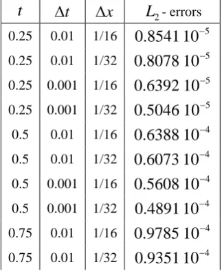
Table (2):

L

₂-errors for the numerical solutions of equation (32).

t

∆

t

∆

x

L

2- errors

0.25 0.01 1/16

0

.

8541

10

−5

0.25 0.01 1/32

0

.

8078

10

−5

0.25 0.001 1/16

0

.

6392

10

−5

0.25 0.001 1/32

0

.

5046

10

−5

0.5 0.01 1/16

0

.

6388

10

−4

0.5 0.01 1/32

0

.

6073

10

−4

0.5 0.001 1/16

0

.

5608

10

−4

0.5 0.001 1/32

0

.

4891

10

−4

0.75 0.01 1/16

0

.

9785

10

−4

0.75 0.001 1/16

₀

_.

₈₉₅₄

₁₀

−4 0.75 0.001 1/32

₀

_.

₈₄₁₆

₁₀

−4 1.0 0.01 1/16

₀

_.

₄₁₃₄

₁₀

−3 1.0 0.01 1/32

₀

_.

₃₀₄₄

₁₀

−3 1.0 0.001 1/16

₀

_.

₂₉₆₁

₁₀

−3 1.0 0.001 1/32

₀

_.

₁₀₂₃

₁₀

−3

Example 3. Let us consider the MKdV equation (32) with the initial condition (28) and the boundary conditions (31) when

p

=

4

,

ε

=

0

.

0000484

,

C

=

0

.

3

,

X

=

8

.

0

and

T

=

1

.

0

. The numerical results are presented in Table (3) (

∆

t

=

0

.

01

and

∆

x

=

0

.

125

).

Table (3)

t

0.25 0. 5 0.75 1.0

2

L

5

10

167524

.

0

−

0

.

903229

10

−5

0

.

980877

10

−5

0

.

173981

10

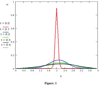
−4

Example 4. We consider the KdVB equation

],

,

0

[

],

,

0

[

,

0

,

,

0

x

X

t

T

u

u

u

u

u

_t

+

_x

−

ν

_xx

+

ε

_xxx

=

ν

ε

>

∈

∈

(33)

with the initial condition (26) and the boundary conditions (31) when

ε

=

0

.

0000484

,

C

=

0.3,

X

=

4.0

and

0

.

4

=

T

. The numerical results for this example applying the multigrid algorithm are presented graphically in fig. 1 for

ν

=

0

.

1

. This figure shows an agreement with the physical expected phenomena given by Conosa and Gazdag [21].

Figure: 1 5. CONCLUSION

6. REFERENCES

[1] Brandt A., Multi-level adaptive solution to boundary-value problem, Math. Comp. 31, 333-390, 1977.

[2] Goldstein C. I., Analysis and application of multigrid preconditioners for singularly perturbed boundary value problems, Siam, Numer. Anal. 26, 1090-1123, 1989.

[3] Dennis J., C., Multigrid method for partial differential equations, Studies in numerical analysis 24, 1984.

[4] Hachbusch W., Multigrid methods and applications, Springer, Berlin, 1984.

[5] Brandt A., Multilevel computations, Marcel Dekker, New York, 1988.

[6] Wesseling P., An introduction to multigrid methods, John Wiley & Sons New York, 1992.

[7] Hassen N. A., Osama E. M. and Fatema H. M., The relaxation schemes for the two dimensional anisotropic partial differential equations using multigrid method, Conf. for Stat., Comp. Scie., Scient & Social Appl. , Cairo 17-22 April, 1995.

[8] Abo Essa Y. M., Amer T. S. and Ibrahim I. A., Numerical treatment of the generalized regularized long-wave equation, Far East Journal of Applied Mathematics 52, 2, 147-154, 2011.

[9] Zabusky N. J. and Kruskal M. D., Interactions of " solitons " in a collision less plasma and the recurrence of initial states, Phys. Rev. Lett, 240-243, 1965.

[10] Greig I. S. and Morris J. LI., A hopscotch method for the Korteweg-de Vries equation, Comput. Phys. 20, 67-80, 1976.

[11] Alexander M. E. and Morris J. LI., Galerkin methods applied to some model equations for non-linear dispersive waves, Comput. Phys. 30, 428-451, 1979.

[12] Sanz-Serna J. M. and Christie I., Petrove-Galerkin methods for non-linear dispersive waves, Comput. Phys. 39, 94-102, 1981.

[13] Schoombie S. W., Central finite difference schemes for non-linear dispersive waves, IMA, Numer. Analysis 2, 95-109, 1982.

[14] Shamardan A. B., Central finite difference schemes for non-linear dispersive waves, Computers Math. Applic. 19, 4, 9-15, 1990.

[15] Chan T. F. and Kerkhoven T., Fourier methods with extended stability intervals for the Korteweg-de Vries equation, SIAM, Numer. Analysis 22, 241-253, 1985.

[16] Su C. H. and Gardner C. S., Derivation of the Korteweg-de Vries and Burgers' equation, Math. Phys. 10, 536-539, 1969.

[17] Grad H. and Hu P. N., Unified shock profile in plasma, Phys. Fluids 10, 2596-2602, 1967.

[18] Grad H. and Hu P. N., Collisional theory of shock and non-linear waves in a plasma, Phys. Fluids 15, 845-864, 1972.

[19] Johnson R. S., A non-linear equation incorporating damping and dispersion, Phys. Fluids Mech. 42, 49-60, 1970.

[20] Johnson R. S., Shallow water waves in a viscous fluid-the undular bore, Phys. Fluids 15, 393-403, 1970.

[21] Conosa J. and Gazdag J., The Korteweg-de Vries Burgers' equation, Comp. Phys. 23, 393-403, 1977.