INVESTIGATION
Population Genetics Inference for
Longitudinally-Sampled Mutants
Under Strong Selection
Miguel Lacerda*,1and Cathal Seoighe†
*Department of Statistical Sciences, University of Cape Town, Rondebosch 7701, South Africa and†School of Mathematics, Statistics and Applied Mathematics, National University of Ireland, Galway, Ireland
ABSTRACTLongitudinal allele frequency data are becoming increasingly prevalent. Such samples permit statistical inference of the
population genetics parameters that influence the fate of mutant variants. To infer these parameters by maximum likelihood, the
mutant frequency is often assumed to evolve according to the Wright–Fisher model. For computational reasons, this discrete model is
commonly approximated by a diffusion process that requires the assumption that the forces of natural selection and mutation are weak. This assumption is not always appropriate. For example, mutations that impart drug resistance in pathogens may evolve under strong selective pressure. Here, we present an alternative approximation to the mutant-frequency distribution that does not make any
assumptions about the magnitude of selection or mutation and is much more computationally efficient than the standard diffusion
approximation. Simulation studies are used to compare the performance of our method to that of the Wright–Fisher and Gaussian
diffusion approximations. For large populations, our method is found to provide a much better approximation to the mutant-frequency distribution when selection is strong, while all three methods perform comparably when selection is weak. Importantly,
maximum-likelihood estimates of the selection coefficient are severely attenuated when selection is strong under the two diffusion models, but
not when our method is used. This is further demonstrated with an application to mutant-frequency data from an experimental study
of bacteriophage evolution. We therefore recommend our method for estimating the selection coefficient when the effective
pop-ulation size is too large to utilize the discrete Wright–Fisher model.
W
ITH the advent of high-throughput sequencing, large and frequent longitudinal samples of segregating alleles are becoming increasingly abundant. The allele-frequency tra-jectories of such samples reflect the combined forces of genetic drift, selection, and mutation and can therefore be used to infer these population genetics parameters. Models of mutant-frequency changes over time are either deterministic or sto-chastic (Rouzineet al.2001). The choice between these models depends on the variance effective population sizeN: the size of a Wright–Fisher population that is identical to the natural pop-ulation in terms of genetic diversity (Kouyoset al.2006). De-terministic models assume that the effective population sizeis infinitely large and therefore that mutant frequencies are not subject to genetic drift, while stochastic models allow the random sampling of variants across generations to
in-fluence the likelihood of mutantfixation and extinction. Most stochastic population genetics models, including the classic coalescent (Kingman 1982), consider the extreme case where selection is so weak that the fate of an allele is de-termined entirely by random genetic drift. Several methods have been developed to infer N based on this assumption (Williamson and Slatkin 1999; Andersonet al.2000; Wang 2001; Berthieret al.2002; Beaumont 2003; Anderson 2005; Jorde and Ryman 2007). There is a growing literature on estimating the selection coefficient,s, using stochastic models of allele-frequency changes (Bollbacket al.2008; Malaspinas
et al.2012; Mathieson and McVean 2013; Federet al.2014; Nishino 2013; Foll et al.2014). Most existing methods im-plicitly assume weak selection by relying on diffusion approx-imations that hold whensis of the order of the reciprocal of
NandNis large. Weak selection is also assumed in the de-terministic paradigm where allele-frequency trajectories are
Copyright © 2014 by the Genetics Society of America doi: 10.1534/genetics.114.167957
Manuscript received July 3, 2014; accepted for publication September 2, 2014; published Early Online September 10, 2014.
Available freely online through the author-supported open access option.
Supporting information is available online athttp://www.genetics.org/lookup/suppl/ doi:10.1534/genetics.114.167957/-/DC1.
1Corresponding author: Department of Statistical Sciences, University of Cape Town,
Rondebosch 7701, South Africa. E-mail: [email protected]
often modeled with a logistic curve obtained in the diffusion limit of the Wright–Fisher and Moran models (Illingworth and Mustonen 2011; Illingworth et al. 2012). All of these approaches are inappropriate when the selective pressure is strong, as is frequently the case, for example, in experimental studies of microbe adaptation and for immune-escape and drug-resistant mutations in intrahost viral populations. Fur-thermore, these methods will provide attenuated estimates of
Nif selection is strong, thereby exaggerating the role of ran-dom genetic drift (Liu and Mittler 2008).
Illingworthet al.(2014) recently presented a method to infer selection of arbitrary magnitude from longitudinal haplotype fre-quencies that are assumed to evolve deterministically. However, their definition of the selection coefficient is not consistent with the population genetics definition of this parameter: for every one offspring contributed to the next generation by the wild type, a mutant contributes 1 +soffspring. Consequently, the authors report estimates of the“selection coefficient”that are ,21, which is not possible in traditional population genetics models.
Recently, Foll et al. (2014) developed an approximate Bayesian computation method to infer selection based on a stochastic model of frequency change. Their two-step ap-proach considers multiple longitudinal samples of segregating alleles from different locations in a genome that are all as-sumed to have the same effective population size. First, the posterior distribution of N is estimated from the frequency trajectories at all genetic loci under the assumption of neutral evolution. The posterior distribution ofsis then inferred for each locus using the previously estimated distribution ofNas a prior. Although the estimation ofsin the second step does not make any assumptions about its magnitude, it is condi-tioned on the estimate of Nthat was inferred assuming no selection. The method is therefore appropriate only if selec-tion is negligible at most loci and genetic drift does not vary between loci. This would not appear to be the case for protein-coding sequences where most positions are usually under strong functional or structural constraints.
Here, we present a simple approximation to the Wright– Fisher process that does not make any assumptions about the magnitude of selection and mutation and is therefore better suited to inferring selection acting on populations evolving under strong selective pressures. We use simulation studies to demonstrate that our approach, based on the delta method of statistics, outperforms the standard and Gaussian diffusion approximations when selection is strong, while all three methods perform comparably when selection is weak. Importantly, maximum-likelihood estimates of the selection coefficient are severely attenuated when selection is strong under the two diffusion models, but not when the delta method is used.
Methods
Model of mutant-frequency evolution
Consider a population of constant effective sizeNcomposed of individuals of two types: wild type and mutant. LetXi2
{0, 1, . . .,N} denote the number of mutants in the popu-lation in generation i. If the mutant frequency evolves according to the Wright–Fisher model, then the conditional number of mutants in the next generation is (Xi+1|Xi=xi) Bin(N,u(xi)/N) with
uðxÞ ¼ð1þsÞxð12aÞ þ ð12xÞb
1þsx ;
where s is the selection coefficient, ais the probability of a mutation from a mutant to the wild type, and b is the probability of a mutation in the reverse direction. This defines a Markov chain {Xn,n= 1, 2,. . .} on the state space
S= {0, 1,. . .,N} with a binomial one-step transition prob-ability matrixℙ.
Of course, we do not observe the number of mutants in the population at each generation. Instead, we collect samples at m time points and observe the mutant frequency yk in a sample of size nk at generationik fork = 1, . . .,m. If the population sizeNis large relative to the sample size
nk, then ðYkjXik¼xikÞ Binðnk;xik=NÞ. The data-generation
process can therefore be described by a hidden Markov model with binomial emissions conditional on the latent number of mutants in the population (Bollback et al.
2008).
The likelihood function of the population genetics param-etersu= {N,s,a,b} under this model is
LðuÞ ¼X Xi1
⋯X Xim
pXi1
Ym
k¼2
pXikþ1Xik;u
Ym
k¼1 pykjXik
;
(1)
wherepðyikXikÞis the binomial sampling probability and
pðXi1Þis a prior distribution for the number of mutants in the first sampled generation. The transition probability distributionpðXikþ1Xik;uÞunder the Wright–Fisher model
is obtained by raising ℙ to the power of ik+1 2 ik. The maximum-likelihood estimates of the population genetics parameters are obtained by maximizing (1) with respect tou.
Approximating the transition probability distribution
Summary:Since there is no analytical solution forpðXikþ1Xik;uÞ
and exponentiation of the (N+ 1)-dimensional transition matrix ℙ is computationally prohibitive when N is large, Bollback et al. (2008) compute the transition function by approximating the Wright–Fisher process with a diffusion pro-cess (Fisher 1922; Wright 1945; Kimura, 1955a,b,c, 1957, 1962, 1964). The diffusion approximation is obtained by mea-suring time in units ofNgenerations and lettingN/Nunder the assumption thats,a,b=O(N21). The consequence of this assumption is that the mean of the transition density will be upwardly biased when |s| . 0 (see Detailssection). Under strong positive and purifying selection, this bias can be signif-icant, as is demonstrated by the simulation studies in the next section.
Norman (1975) relaxed this assumption with a Gaussian diffusion approximation in which mutant frequencies are centered about their deterministic trajectory with asymptot-ically normal deviations attributable to random genetic drift. The approximation still requires that the selection coeffi -cient and mutation rates tend to zero as N / N, but assumes that the variability in mutant-frequency changes dies off faster in the limit. When selection or mutation is strong, the mean and variance of the Gaussian transition density will be biased.
While the moments derived under the assumptions of the Gaussian diffusion will be inappropriate when selection is strong, a normal approximation of the transition distribution is still reasonable. The skewness in the mutant-frequency distribution that results from stochastic loss will not develop for mutants under strong positive selection (Ns1) once the mutant has reached a frequency of1/Nsin the popu-lation (Maynard Smith 1971). In this case, the mutant fre-quency will track its expected value closely with small, symmetric departures due to genetic drift. We used the delta method to approximate the mean and variance of the Wright– Fisher process with a system of nonlinear difference equations that do not make any assumptions about the magnitude ofs,
aorb(seeDetailssection). These equations can be solved numerically and the transition density can then be approxi-mated by a Gaussian distribution with these two moments. The implementation of this method is extremely efficient; it requires only the routine computation of the Gaussian density, as opposed to the standard diffusion approximation, which re-quires specialized numerical techniques to solve Kolmogorov’s forward equation.
Details:Here, we provide a detailed description of the three methods used to approximate the transition probability function.
Diffusion approximation: The diffusion approximation to the Wright–Fisher process was first considered by Fisher (1930) and Wright (1931) and later substantially extended by Kimura (1955a,b,c, 1957, 1962, 1964). To approximate the discrete-state, discrete-time Wright–Fisher model with a diffusion process, it is necessary to scale the state space and time so that they are both approximately continuous. If
Xn represents the proportion of mutants in a population of effective sizeNat generationn, then the state space will be approximately continuous on [0, 1] ifNis large. Similarly, if time is measured in units ofNgenerations such that changes occur in steps of sizeN21, then it too will converge to a con-tinuous measure in the limit asN/N. Hence, the diffusion approximation holds whenNis large. Fortunately, it is pre-cisely in this context that the approximation is required to overcome the computational burden of exponentiating the large transition matrix,ℙ, of the discrete Wright–Fisher Markov chain.
Let {Xt,t$0} denote the proportion of mutants at time
tmeasured in units ofNgenerations in the limit asN/N. The diffusion process {Xt} is defined by its infinitesimal mean
mðxÞ ¼ lim
N/NE½dXtjXt ¼x
dt
¼ lim N/N
Nsxð12xÞ2Naxð1þsÞ þNbð12xÞ
1þsx
¼hlim N/NNs
i
xð12xÞ2
lim N/NNa
x
þ
lim N/NNb
ð12xÞ (2)
and infinitesimal variance
s2ðxÞ ¼ lim N/NVar
dXtjXt ¼x dt
¼ lim
N/N
ð1þsÞxð12aÞ þ ð12xÞb
1þsx
3
12ð1þsÞxð12aÞ þ ð12xÞb 1þsx
¼xð12xÞ
(see, for example, Ewens 2004). Importantly, the last line in each of the above derivations requires thats,a,b=O(N21), so thatNs,Na,andNbare constants ands,a,andb/0 as
N/N. To understand the consequences of this assumption for inference, consider a population that evolves as a Wright– Fisher process without mutation. The expected change in the mutant frequency in one generation is then
sxð12xÞ
1þsx ;
while the diffusion approximation of this change is
mðxÞdt¼sxð12xÞ:
The expected mutant frequency therefore evolves according to a logistic function under the diffusion approximation. This will be a good approximation only for |s| 0, but will be upwardly biased for strong positive or negative selection. This implies that the mutant-frequency distribution will drift over toward fixation too rapidly under strong positive selection (s 0) and will move toward loss too slowly under strong negative selection (s0). The diffusion approximation will therefore lead to attenuated estimates of |s| when selection is strong.
Given the infinitesimal mean and variance, the transition density f(x, t) [ p(Xt|X0, N, s, a, b) is the solution to Kolmogorov’s forward equation
@
@tfðx;tÞ ¼ 2
@
@xmðxÞfðx,tÞ þ
1 2
@2 @x2s
2ðxÞfðx,tÞ:
The analytical solution to this equation was derived in a series of articles by Kimura (1955a,b,c 1957) for the special cases of pure random drift and random drift with selection and no
mutation. The solutions in these special cases are extremely complex, involving infinite sums of Gegenbauer polynomials. Consequently, numerical methods for partial differential equa-tions are typically employed to solve for the transition density
f(x,t). We used the exponentiallyfitted difference scheme of Duffy (1980), which is better suited than the Crank–Nicolson method employed by Bollbacket al.(2008) to problems with singular initial conditions. When the discrete transition dis-tribution is approximated with a continuous density function such asf(x,t), the summations in (1) must be replaced with integrations. We used the trapezoidal rule to perform all inte-grations numerically.
Gaussian diffusion:The assumption thatNs=O(1) is not appropriate in a regime where selection dominates genetic drift. Norman (1975) considered the case where stochastic changes due to genetic drift die off faster than the effects of selection and mutation in the limit asNe/Nande/0, wheree = max{|s|,a,b}. With time measured in units of
e21generations, the mean and variance of an infinitesimal
change in the mutant frequency are then
mðxÞ ¼lim e/0
e21sxð12xÞ2e21axþe21bð12xÞ 1þsx
¼
lim e/0e
21s
xð12xÞ2
lim e/0e
21a
x
þ
lim e/0e
21b
ð12xÞ (3)
and
s2ðxÞ ¼ lim
e/0; Ne/N
ð1þsÞxð12aÞ þ ð12xÞb
1þsx
3
12ð1þsÞxð12aÞ þ ð12xÞb 1þsx
1
Ne
¼ lim
Ne/N
xð12xÞ Ne ;
respectively. The standard diffusion is a special case where
e =N21. Note that the assumption of weak selection and mutation through e / 0 leads to the simplification in the second line of both equations. In particular, we note that the infinitesimal mean will suffer from the same bias as that of the standard diffusion approximation when selection is strong. The Gaussian diffusion is obtained by assuming that
Ne /NasN/ Nande /0 such that the variance of a displacement tends to zero faster than its expected value in the limit. Under these conditions, Norman (1975) showed that the transition density after n generations with initial mutant frequency p is approximately Gaussian with mean
f(ne,p) and varianceg(ne,p)/Ne, wherefis the solution to
d
dt fðt;xÞ ¼m
fðt;xÞ
subject tof(0,x) =xandgis given by
gðt;xÞ ¼ Z t
0 exp
2
Z t
u m9
fðj;xÞ dj
nfðu;xÞ du;
wheren(x) =x(12x). Here, we are interested in the case where selection is stronger than mutation, that is,e= |s|. In this case, the transition density of the Gaussian diffusion afterngenerations has mean
E½XnjX0¼p ¼
p pþ ð12pÞe2sn
and variance
Var½XnjX0¼p
¼pð12pÞe
nshp2e2nsþ ð122p22nspðp21ÞÞens2ðp21Þ2i
Ns½1þpðens21Þ4 :
Obtaining the transition density under the Gaussian diffu-sion is therefore computationally straightforward. Note that the expected mutant frequency is described by the same logistic function as the standard diffusion approximation, but that the dispersion about this deterministic trajectory will necessarily be symmetric.
Delta method: The moments of the transition densities under both the standard and Gaussian diffusion approxima-tions were derived under the assumption of weak selection and mutation. We obtained approximate expressions for the mean and variance of this distribution without making any assumptions about the strength of selection and mutation using the delta method (see, for example, Rice 2007, Chap. 4). For a random variable Xwith mean mand variances2,
the mean and variance of a function f(X) can be approxi-mated withfirst-order Taylor expansions aboutm:
E½fðXÞ fðmÞ
Var½fðXÞ f9ðmÞ 2s2:
If {Xn,n= 0, 1, . . .} is a Wright–Fisher process, the mean
mn[E[Xn|X0] and variances2n[Var½XnjX0of the transition function can therefore be approximated as
mn¼E½E½XnjXn21X0
¼E
ð1þsÞXn21ð12aÞ þ ð12Xn21Þb 1þsXn21
X0
ð1þsÞmn21ð12aÞ þ ð12mn21Þb 1þsmn21
and
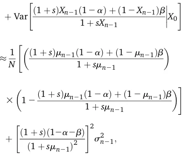
s2 n¼E
Var½XnjXn21X0 þVar
E½XnjXn21X0
¼1
NE "
ð1þsÞXn21ð12aÞ þ ð12Xn21Þb 1þsXn21
3
12ð1þsÞXn21ð12aÞ þ ð12Xn21Þb 1þsXn21
X0
#
þVar
"
ð1þsÞXn21ð12aÞ þ ð12Xn21Þb 1þsXn21
X0
#
1
N "ð
1þsÞmn21ð12aÞ þ ð12mn21Þb 1þsmn21
3
12ð1þsÞmn21ð12aÞ þ ð12mn21Þb 1þsmn21
#
þ
"
ð1þsÞð12a2bÞ
ð1þsmn21Þ2 #2
s2 n21;
respectively. Hence we obtain a system of nonlinear re-currence equations that can be solved numerically for the mean and variance of the transition distribution given an initial frequencyX0=p. For large populations with strong selection or mutation, the transition density can then be approximated by a Gaussian distribution with these moments. The usual delta method of statistics uses a second-order Taylor series approximation for the mean. We considered this and a second-order Taylor series approximation for the variance. We investigated the behavior of the resulting systems of equations empirically for different values ofs,N, and p with a = b = 0. We found that the system began to oscillate when p , 1/Ns for s . 0 when second-order approximations were used for either the mean only or the mean and the variance, but not whenfirst-order approxima-tions were used for both of these moments. Interestingly, whenP,1/Ns, the frequency of the mutant is too low to ensure its ultimatefixation and the resulting transition dis-tribution will involve singularities at the boundaries. Clearly, such a mutant-frequency distribution cannot be accurately modeled with a Gaussian density. We ran all of our simula-tions using both the first-order approximation to the mean and variance and the second-order approximation to the mean. Although the true and inferred deterministic paths were indistinguishable when a second-order approximation was used for the mean, the improvement in accuracy did not substantively affect our simulation results. We have included the transition densities that we obtained with the second-order approximation to the mean inSupporting Information,
Figure S1. Consequently, we report only the results obtained with thefirst-order approximations to the mean and variance, which did not lead to spurious oscillations for any of the parameter values investigated.
Implementation
All computer code was written in the R Language and Environment for Statistical Computing and is freely available from the corresponding author. The maximum-likelihood estimates were obtained with a steepest-ascent hill-climbing algorithm and were checked by plotting the likelihood surface when possible.
Results
Comparison of model approximations
For small N, the exact transition distribution of a discrete Wright–Fisher process can be evaluated numerically. We compared the approximate distribution obtained with each of the above three methods to the exact distribution forN= 100, 1000, and 5000 after n= 5, 10, and 20 generations starting with an initial mutant frequency ofp= 0.1, 0.5, and 0.9. For each of these 27 combinations, we computed the mutant-frequency distribution for selection coefficients of 0, 60.001, 60.01, 60.1, 60.3, and 60.5 and no mutation. The complete set of results is presented inFigure S1.
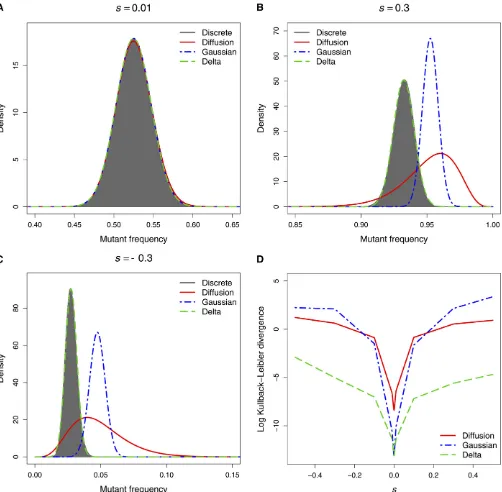
As expected all three methods provided an excellent approximation to the exact transition distribution when selec-tion was weak (|s|,0.01) and the population size was large (see Figure 1A, for example). When N= 5000, the standard and Gaussian diffusion approximations performed poorly under strong selection (|s|.0.1). As is evident from Figures 1, B and C, the approximate transition distributions obtained with these methods are located too far to the right, a direct consequence of the assumption thats=O(N21) (seeMethods). In contrast, our delta method approach provided an excellent approximation to the true distribution when the population size was large, irre-spective of the strength of selection. Figure 1D, which plots the Kullback–Leibler divergence of each approximate distribution from the exact distribution, demonstrates the superior perfor-mance of our method compared to the standard and Gaussian diffusion approximations under strong positive and negative selection in a large population with an initial mutant frequency of 0.5. For large populations with initial mutant frequencies of 0.1 and 0.9, the delta method performed particularly well when there was strong selection away from the absorbing boundaries at 0 and 1, respectively (see the Kullback–Leibler divergence plots inFigure S1).
When the population size was small (N= 100), the two methods that approximated the transition distribution with a Gaussian density performed less well compared to the standard diffusion approximation when selection was weak (see Figure S1). This result is unsurprising since random departures from the mean mutant frequency will be approx-imately normal only when the population size is large and selection is strong enough to prevent stochastic loss. When genetic drift dominates selection, the mutant-frequency dis-tribution will develop singularities and skewness that cannot be captured by the Gaussian density. Interestingly, the stan-dard diffusion model, which is derived in the limit asN/N, performs remarkably well whenNis this small, provided, of course, that selection is weak. This is in agreement with the
findings of Ewens (1963). When selection is strong, all three methods provide rather poor approximations to the true den-sity if the population size is small (seeFigure S1). However, no approximation is necessary when the population size is small, since the exact Wright–Fisher transition distribution can then be computed numerically from the transition matrix and initial mutant-frequency distribution.
Simulations
To assess how the three approximations affect population genetic inferences, we simulated 1000 realizations of a Wright–Fisher process with selection and no mutation for 20 generations. A relatively small effective population size of N = 1000 was used, because the matrix multiplications required to simulate a discrete Wright–Fisher process were computationally bur-densome for larger values ofN. For each simulated process,
Nandswere estimated by maximizing the likelihood function
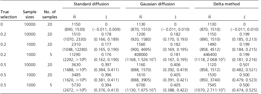
(1) with a uniform prior distribution for the initial popula-tion mutant frequency using each of the three approxima-tions to the transition distribution. As a check that the three approaches perform as expected, the data were initially simulated withs= 0 andp= 0.5, and the parameters were estimated from large samples of size 10000 observed at all 20 generations. Under these conditions, all three methods performed similarly, yielding unbiased estimates,N^ and^s, of N and s with similar standard errors (see Table 1 and
Figure S2).
Figure 1 The exact transition distribution of the Wright–Fisher process and its three approximations aftern= 10 generations whenN= 5000 andp= 0.5. (A) Weak selection (s= 0.01). (B) Strong positive selection (s= 0.3). (C) Strong negative selection (s=20.3). (D) Kullback–Leibler divergence from the exact distribution.
For the remaining simulations, we considered selection coefficients ofs = 0.2 ands= 0.5 with initial mutant fre-quencies of p = 0.05 and P= 0.01, respectively. Bollback
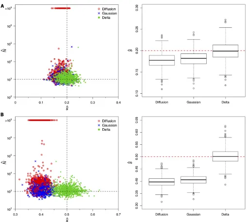
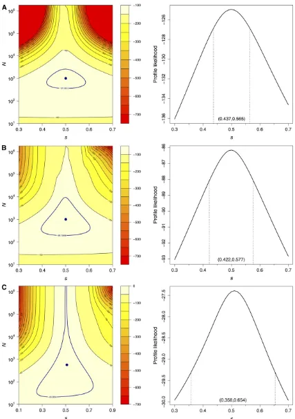
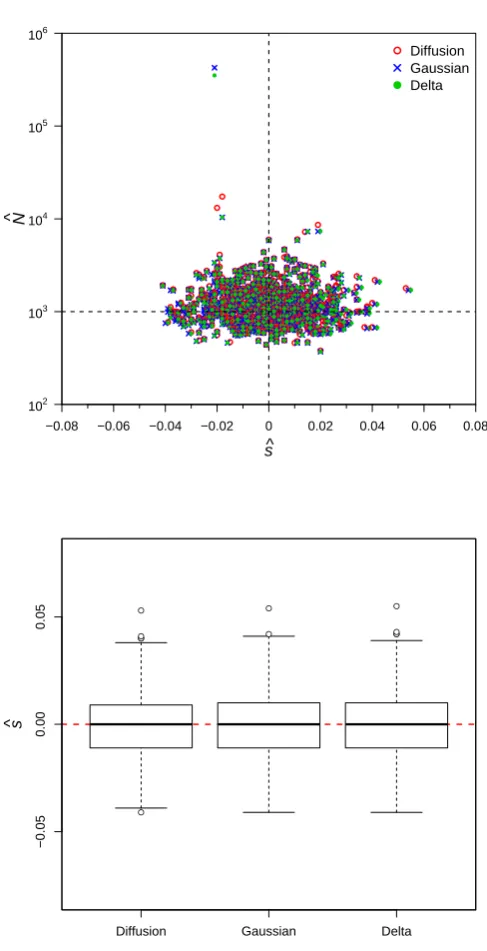
et al.(2008) inferred a selection coefficient of 0.43 for the C206U mutation of the bacteriophage MS2 using the stan-dard diffusion approximation to the transition distribution. Given the results of the previous subsection, we would ex-pect this estimate to be downwardly biased. To assess the severity of this bias using simulations, we first considered the ideal case in which large samples of 10000 sequences were observed at every generation for all 20 generations. Although these conditions may be unrealistic in practice, the purpose of this simulation study was to establish benchmark performances to serve as a basis for comparison when these ideal conditions are not met. We found that the Gaussian diffusion and delta methods provided reasonable maximum-likelihood estimates (MLEs) of Nwith interquartile ranges that included the true value of 1000 (see Table 1). The estimates of N obtained with the standard diffusion were more variable than those of the other two methods, and the median and interquartile range were upwardly biased. The selection coefficient s was underestimated with both the standard and Gaussian diffusion approximations. The bias was particularly severe when s = 0.5, with all of the 1000 MLEs falling below the true value for the standard and Gaussian diffusion approximations (median^svalues of 0.397 and 0.406, respectively). Our delta method approxi-mation, on the other hand, yielded estimates ofsthat were centered about the true value and only slightly more vari-able than those of the other two methods (see Tvari-able 1 and Figure 2).
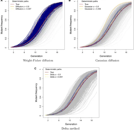
Approximately one-third of the simulated data sets pro-duced MLEs ofNin excess of 100 million when the standard diffusion approximation was employed with s = 0.5 (see Figure 2). These corresponded to data sets where the mu-tant frequency rose rapidly towardfixation (see Figure 3A).
For a given level of selection, a large population size in-creases the expected displacement of the mutant frequency in an infinitesimal amount of time under this model (see Equation 2 in Methods). The larger estimates of N were therefore compensating for the downwardly biased estimates ofs when the mutant-frequency trajectory rose sharply. In-terestingly, such large estimates ofNwere not observed un-der the Gaussian diffusion approximation, even though ^s
was also downwardly biased under this model. This is be-cause the infinitesimal mean of the Gaussian diffusion is not a function ofNand therefore increasing the effective pop-ulation size would not help to explain the rapid rise in mu-tant frequency (see Equation 3 in Methods). Instead, the simulated trajectories that yielded large N estimates with the Gaussian diffusion and delta methods closely tracked the true deterministic path (that is, the expected values of the discrete Wright–Fisher process used to simulate the data; see Figures 3, B and C). Note that the deterministic paths implied by the standard and Gaussian diffusion mod-els rise much more rapidly than the true deterministic path of the data-generating process when s = 0.5. The down-wardly biased estimates ofsensure that the deterministic tra-jectory based on the median^srepresents the center of the data in both cases (see Figures 3, A and B). This was not the case for our delta method approximation, where the true and inferred deterministic paths were very similar (see Figure 3C).
We conducted two further simulation studies to assess the effect of reducing the sample size and sampling frequency. In the first of these, the sample size was reduced to 1000 sequences per generation. In the second study, we assumed that the smaller samples were observed at only five equally spaced time points rather than for all 20 generations. The resulting estimates of N and s are summarized in Table 1,
Figure S3, andFigure S4. As expected, reducing the sample size and, particularly, the sampling frequency increased the variability of the estimates of N. Interestingly though, the Table 1 Medians of the maximum-likelihood estimates ofNandsobtained in 1000 data sets simulated under the conditions given in the
first three columns
Standard diffusion Gaussian diffusion Delta method
True selection
Sample sizes
No. of
samples N^ ^s N^ ^s N^ ^s
0 10000 20 1150 0 1130 0 1130 0
(890, 1530) (20.011, 0.009) (870, 1510) (20.011, 0.010) (870, 1510) (20.011, 0.010)
0.2 10000 20 1510 0.178 1200 0.182 1150 0.199
(1070, 2330) (0.166, 0.189) (920, 1580) (0.170, 0.193) (890, 1510) (0.185, 0.213)
0.2 1000 20 2310 0.177 1560 0.182 1490 0.199
(1048, 12280) (0.165, 0.190) (900, 4695) (0.169, 0.195) (858, 4512) (0.184, 0.215)
0.2 1000 5 11290 0.176 408000 0.181 446400 0.199
(2292,.108) (0.162, 0.190) (1168, 1.526107) (0.167, 0.195) (1118, 2.068107) (0.181, 0.216)
0.5 10000 20 3630 0.397 1160 0.406 1120 0.501
(1688,.108) (0.384, 0.411) (888, 1570) (0.392, 0.419) (858, 1512) (0.482, 0.521)
0.5 1000 20 3485 0.396 1610 0.405 1530 0.500
(1620,.108) (0.381, 0.411) (888, 3905) (0.391, 0.421) (850, 3740) (0.479, 0.523)
0.5 1000 5 5730 0.394 6700 0.405 7545 0.500
(2672,.108) (0.376, 0.413) (1130, 1.675107) (0.388, 0.422) (1070, 2.711107) (0.474, 0.525)
In all cases, the true population size wasN= 1000. The interquartile ranges are indicated in parentheses.
variability of ^s did not increase notably in either of these cases. However, reducing the sampling frequency did have a profound effect on likelihood intervals for (N,s). As illustrated in Figure 4 for one simulated data set withs= 0.5, the 95% likelihood interval based on the delta method widened con-siderably when the sampling frequency was reduced fourfold. This expansion was particularly conspicuous along theN di-mension, since fewer sample points implies less information on the genetic drift of the process. This was also noted by Malaspinaset al.(2012) in their simulations. There was also a more notable widening of the 95% profile likelihood inter-vals forswhen fewer samples were taken compared to when the size of each sample was reduced.
Application
We applied our method to a mutant-frequency trajectory from an experimental study of bacteriophage adaptation (Bollback and Huelsenbeck 2007). Briefly, this study evolved large populations (census size of 5 3107) of the
bacterio-phage MS2 for 100 generations at elevated temperatures and tracked nucleotide substitutions occurring during adap-tation. Since the mutants in this study evolved under strong selective pressure, we anticipated that our delta method approach would provide more accurate estimates of the population genetics parameters than the standard diffu-sion approximation.
Figure 2 MLEs forNandsobtained in 1000 data sets simulated withN= 1000 and (A)s= 0.2 and (B)s= 0.5. Estimates were based on the mutant frequencies observed in samples of size 10000 taken every generation for 20 generations of the process, starting with an initial population mutant frequency ofp= 0.05 in A andp= 0.01 in B.
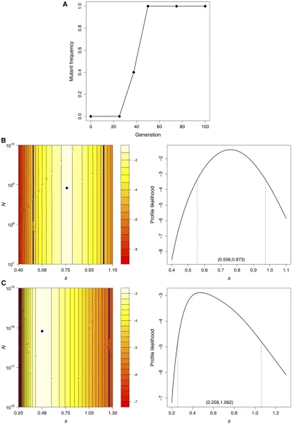
We chose to apply our method to the U1685C mutation in experimental line 3, which rose rapidly in frequency once it appeared and is therefore likely to have a particularly large selection coefficient (see Figure 5A). The frequency of this mutation was measured at six time points based on 10 sequences at each time point (9 sequences at the second time point). Note that the sample size in this application is much smaller than that which we considered in our simula-tion studies, and we therefore expect much wider confi
-dence intervals for the parameters. Since no mutants were observed until after the second time point, we assumed that the mutant arose only thereafter and used an informative prior with a point mass at zero for the population mutant frequency at generation 25. The mutation rates from C to U (a) and from U to C (b) were both set to 1
331023 (Drake
1993).
The log-likelihood surface for U1685C obtained with our delta method approach is plotted in Figure 5B. The MLE of Figure 3 Trajectories with largeNestimates based on the (A) Wright–Fisher diffusion model, (B) Gaussian diffusion model, and (C) delta method. Navy lines indicate data sets withN^.108in A andN^.5 000 in B and C. The deterministic path based on the true data-generating process withs= 0.5 and N= 1000 is indicated with a red line. The deterministic path based on the model is indicated with an orange line fors= 0.5 and with a yellow line for the median value of^s.
Figure 4 Log-likelihood surfaces (left) and profile likelihoods fors(right) obtained with the delta method for a selected simulated data set withN= 1000 ands= 0.5. (A) Samples of size 10,000 observed every generation for 20 generations. (B) Samples of size 1000 observed every generation for 20 generations. (C) Samples of size 1000 observed every fourth generation for 20 generations. Navy points indicate MLEs and navy contour lines indicate 95% likelihood regions. Dashed lines on the profile likelihood panels mark the 95% likelihood intervals forsgiven in parentheses.
Figure 5 Data and results for the bacteriophage U1685C mutation. (A) Mutant frequency trajectory. The log-likelihood surface (left) and profile likelihood fors(right) were computed with the (B) delta method and the (C) Wright–Fisher diffusion approximation. The navy points on the log-likelihood surfaces indicate the MLEs and the navy contour lines indicate the 95% log-likelihood regions. Dashed lines on the profile likelihood plots mark the 95% likelihood intervals forsgiven in parentheses.
the effective population size was N^ ¼8:323108, although
it is clear from the likelihood surface plot that this parameter cannot be reliably estimated from these data (the likelihood surface was flat along theNdimension for Nvalues in the range 104–1019). Indeed, this nucleotide site was observed to
be polymorphic only at one time point and it is therefore not possible to confidently infer the extent of genetic drift. In contrast, the trajectory does contain information about the selection coefficient. We obtained a large MLE of^s¼0:759
with a 95% profile likelihood interval of (0.559, 0.973) using the delta method (see Figure 5B).
As expected, the MLE based on the standard diffusion approximation was substantially smaller at^s¼0:475 and
was less than the lower bound of the 95% likelihood interval obtained with the delta method (see Figure 5C). The corre-sponding profile likelihood interval based on the diffusion approximation was also much wider at (0.258, 1.062). As we observed in our simulation studies, the MLE of the effec-tive population size obtained with the diffusion approxima-tion,N^ ¼8:1931017, was much larger than that obtained
with the delta method and appears to compensate for the downwardly biased estimate ofs. However, as with the delta method, this parameter could not be reliably estimated with the diffusion approximation.
Discussion
Developments in ultra-deep sequencing technologies have greatly enhanced our ability to track changes in the genetic diversity of measurably evolving populations over time. Large genetic samples collected at several time points permit efficient statistical inference of the population genetics parameters that govern the fate of mutant variants.
In this article, we considered a stochastic model of mutant-frequency evolution that can be used to infer the effective population size, selection coefficient, and mutation rates from temporal allele-frequency data using the method of maxi-mum likelihood. In this hidden Markov model, the observed mutant frequencies are obtained through binomial sampling from a population in which the mutant frequency evolves according to the Wright–Fisher process. Because there is no simple analytical expression for the transition distribution of this process and its numerical evaluation is computationally prohibitive for large effective population sizes, the Wright– Fisher model is commonly approximated with a diffusion pro-cess (Fisher 1922; Wright 1945; Kimura, 1955a,b,c, 1957, 1962, 1964). However, this approximation assumes that the forces of selection and mutation are weak. This assumption is not always appropriate. For example, mutations in intrahost viral populations are likely to be under strong selection to evade the immune response and drug therapy, and microbes are often subjected to strong selective pressures in experi-mental studies of adaptation. Moreover, the assumption of weak selection and mutation is often overlooked in the liter-ature, although, as we have demonstrated, it has profound implications for inferences.
Norman (1975) derived an alternative approximation to the Wright–Fisher process, known as the Gaussian diffusion, in which the effects of selection and mutation die off less rapidly compared to genetic drift as the population size gets larger and the selection and mutation parameters tend to zero. Here, we developed a novel approximation that is ex-tremely accurate for a population with a large effective size. Like Norman (1975), we approximate the transition distri-bution with a Gaussian density, but use the delta method of statistics to derive a set of recurrence equations for the mean and variance of this distribution without making any assump-tions about the strength of selection and mutation.
By comparing the approximate transition densities to the exact distribution, we showed that all three methods perform well when the effective population size is large and selection is weak. However, the quality of the standard and Gaussian diffusion approximations was severely compromised when selection was strong. In both cases, the transition distribu-tion shifts too rapidly toward mutantfixation under strong positive selection and too slowly toward mutant loss under strong purifying selection. In contrast, our approximation was remarkably accurate for large effective population sizes irrespective of the strength of selection.
The accuracy of the approximation has important con-sequences for estimates of the selection coefficient. Using simulated Wright–Fisher trajectories, we demonstrated that maximum-likelihood estimates of the selection coefficient are severely attenuated when selection is strong using either the standard or Gaussian diffusion approximations to the transition distribution. On the other hand, our delta method approach yielded unbiased estimates of the selection coeffi -cient, irrespective of the sampling frequency or sample size. We applied our method to infer selection for a mutant in an experimental study of bacteriophage adaptation under heat stress. As expected from our simulation study, the estimated selection coefficient of 0.759 obtained with the delta method was much larger than the estimate of 0.475 obtained with the standard diffusion approximation.
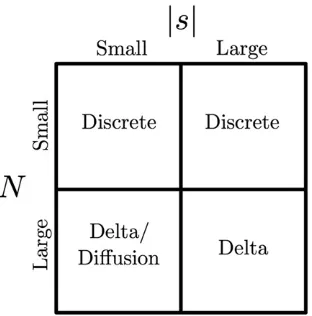
Frequent sampling is needed to obtain robust and precise parameter estimates. In our simulation study, we demonstrated that reducing the sampling frequency leads to wider confi -dence regions, particularly in the direction of the effective population size. Indeed, we were unable to reliably infer this parameter in our bacteriophage application where the nucleotide site was observed to be polymorphic at only one time point. Interestingly though, this mutant-frequency trajectory still contained enough information with which to obtain a bounded likelihood interval for the selection coefficient. Given sufficient time points, it would also be possible to allow the selection coefficient to vary over time, which often occurs in natural populations. Ignoring time-varying selection could lead to attenuated estimates of the effective population size. Figure 6 summarizes the appropriate statistical methods for different regions the (N,s) parameter space. When the effective population size is small (N,5000), exponentia-tion of the one-step transiexponentia-tion probability matrix of the
discrete Wright–Fisher Markov chain is computationally fea-sible and should be used for inferences. For mutants evolving under weak selection (|s|,0.01) in populations with a large effective size (N.5000), either of the diffusion approxima-tions or the delta method approach can be used for accurate inferences. However, we recommend the delta method over the standard diffusion approximation as it is computationally far more efficient. Finally, when the effective population size is large and selection is strong, only our delta method ap-proach will provide an unbiased estimate of the selection coefficient.
In practice, we may not havea prioriinformation on the magnitudes of the parameters for a given data set. In this case, one could begin by first optimizing the likelihood based on the discrete Wright–Fisher model over small values ofN(N,5000). If the optimal (N,s) point lies on the upper boundary of N, then one would proceed to perform the optimization over larger values ofNusing the delta method approximation. Alternatively, one could plot the likelihood surface using the appropriate method in each region of the parameter space.
Literature Cited
Anderson, E. C., 2005 An efficient Monte Carlo method for esti-matingNefrom temporally spaced samples using a
coalescent-based likelihood. Genetics 170: 955–967.
Anderson, E. C., E. G. Williamson, and E. A. Thompson, 2000 Monte Carlo evaluation of the likelihood for Ne from
temporally spaced samples. Genetics 156: 2109–2118. Beaumont, M. A., 2003 Estimation of population growth or
de-cline in genetically monitored populations. Genetics 164: 1139– 1160.
Berthier, P., M. A. Beaumont, J.-M. Cornuet, and G. Luikart, 2002 Likelihood-based estimation of the effective population size using temporal changes in allele frequencies: a genealogical approach. Genetics 160: 741–751.
Bollback, J. P., and J. P. Huelsenbeck, 2007 Clonal interference is alleviated by high mutation rates in large populations. Mol. Biol. Evol. 24(6): 1397–1406.
Bollback, J. P., T. L. York, and R. Nielsen, 2008 Estimation of 2Nes
from temporal allele frequency data. Genetics 179: 497–502.
Drake, J. W., 1993 Rates of spontaneous mutation among rna viruses. Proc. Natl. Acad. Sci. USA 90(9): 4171–4175. Duffy, D. J., 1980 Uniformly convergent difference schemes for
prob-lems with a small parameter in the leading derivative. Ph.D. the-sis, Trinity College, Dublin, Ireland.
Ewens, W. J., 1963 Numerical results and diffusion approxima-tions in a genetic process. Biometrika 50(3/4): 241–249. Ewens, W. J., 2004 Mathematical Population Genetics: Theoretical
Introduction, Ed. 2. Springer-Verlag, New York.
Feder, A. F., S. Kryazhimskiy, and J. B. Plotkin, 2014 Identifying signatures of selection in genetic time series. Genetics 196: 509– 522.
Fisher, R. A., 1922 On the dominance ratio. Proc. R. Soc. Edinb. 42: 321–341.
Fisher, R. A., 1930 The Genetical Theory of Natural Selection. Ox-ford University Press, OxOx-ford.
Foll, M., Y.-P. Poh, N. Renzette, A. Ferrer-Admetlla, C. Banket al., 2014 Influenza virus drug resistance: A time-sampled popula-tion genetics perspective. PLoS Genet. 10(2): e1004185. Illingworth, C. J. R., and V. Mustonen, 2011 Distinguishing driver
and passenger mutations in an evolutionary history categorized by interference. Genetics 189: 989–1000.
Illingworth, C. J. R., L. Parts, S. Schiffels, G. Liti, and V. Mustonen, 2012 Quantifying selection acting on a complex trait using allele frequency time series data. Mol. Biol. Evol. 29(4): 1187–1197.
Illingworth, C. J. R., A. Fischer, and V. Mustonen, 2014 Identifying selection in the within-host evolution of influenza using viral sequence data. PLOS Comput. Biol. 10(7): e1003755.
Jorde, P. E., and N. Ryman, 2007 Unbiased estimator for genetic drift and effective population size. Genetics 177: 927–935. Kimura, M., 1955a Random genetic drift in multi-allelic locus.
Evolution 9(4): 419–435.
Kimura, M., 1955b Solution of a process of random genetic drift with a continuous model. Proc. Natl. Acad. Sci. USA 41(3): 144– 150.
Kimura, M., 1955c Stochastic processes and distribution of gene frequencies under natural selection. Cold Spring Harb. Symp. Quant. Biol. 20: 33–53.
Kimura, M., 1957 Some problems of stochastic processes in ge-netics. Ann. Math. Stat. 28(4): 882–901.
Kimura, M., 1962 On the probability offixation of mutant genes in a population. Genetics 47: 713–719.
Kimura, M., 1964 Diffusion models in population genetics. J. Appl. Probab. 1(2): 177–232.
Kingman, J., 1982 The coalescent. Stochast. Proc. Appl. 13(3): 235–248.
Kouyos, R. D., C. L. Althaus, and S. Bonhoeffer, 2006 Stochastic or deterministic: What is the effective population size of HIV-1? Trends Microbiol. 14(12): 507–511.
Liu, Y., and J. Mittler, 2008 Selection dramatically reduces effec-tive population size in HIV-1 infection. BMC Evol. Biol. 8(1): 133.
Malaspinas, A.-S., O. Malaspinas, S. N. Evans, and M. Slatkin, 2012 Estimating allele age and selection coefficient from time-serial data. Genetics 192: 599–607.
Mathieson, I., and G. McVean, 2013 Estimating selection coeffi -cients in spatially structured populations from time series data of allele frequencies. Genetics 193: 973984.
Maynard Smith, J., 1971 What use is sex? J. Theor. Biol. 30(2): 319–335.
Nishino, J. 2013 Detecting selection using time-series data of al-lele frequencies with multiple independent reference loci. G3 (Bethesda) 3: 2151–2161.
Norman, F., 1975 Approximation of stochastic processes by Gaussian diffusions, and applications to Wright–Fisher genetic models. SIAM J. Appl. Math. 29(2): 225–242.
Figure 6 Parameter space with appropriate method of inference.
Rice, J. A., 2007 Mathematical Statistics and Data Analysis, Ed. 3. Duxbury Press, Belmont, California.
Rouzine, I. M., A. Rodrigo, and J. M. Coffin, 2001 Transition between stochastic evolution and deterministic evolution in the presence of selection: general theory and application to virology. Microbiol. Mol. Biol. Rev. 65(1): 151–185.
Wang, J., 2001 A pseudo-likelihood method for estimating effec-tive population size from temporally spaced samples. Genet. Res. 78: 243–257.
Williamson, E. G., and M. Slatkin, 1999 Using maximum likeli-hood to estimate population size from temporal changes in al-lele frequencies. Genetics 152: 755–761.
Wright, S., 1931 Evolution in Mendelian populations. Genetics 16: 97–159.
Wright, S., 1945 The differential equation of the distribution of gene frequencies. Proc. Natl. Acad. Sci. USA 31: 382–389.
Communicating editor: L. M. Wahl
GENETICS
Supporting Information
http://www.genetics.org/lookup/suppl/doi:10.1534/genetics.114.167957/-/DC1
Population Genetics Inference for
Longitudinally-Sampled Mutants
Under Strong Selection
Miguel Lacerda and Cathal Seoighe
Supplementary Material
Figure S1: This series of plots illustrates the approximations to the discrete
Wright-Fisher mutant frequency distribution for various values of the selection coefficient
s
,
effective population size
N
, initial mutant frequency
p
and number of generations
n
.
The true, discrete Wright-Fisher mutant frequency distribution is shown in grey and
is rescaled such that the area under the curve is equal to one. The standard diffusion
approximation is indicated in red and the Gaussian diffusion approximation is given in
blue. The approximate distributions obtained with the delta method are indicated in
green and orange for the first-order and second-order Taylor approximations of the mean,
respectively (see Methods). The plot at the bottom right of each page shows the log
Kullback-Leibler divergence from the true Wright-Fisher mutant frequency distribution
as a function of the selection coefficient for each of the approximations.
N
= 100,
p
= 0
.
1,
n
= 5
0.0 0.2 0.4 0.6 0.8 1.0
0
20
40
60
80
100
120
140
Mutant frequency
Density
s=−0.5
0.0 0.2 0.4 0.6 0.8 1.0
0
10
20
30
40
50
Mutant frequency
Density
s=−0.3
0.0 0.2 0.4 0.6 0.8 1.0
0
2
4
6
8
10
Mutant frequency
Density
s=−0.1
0.0 0.2 0.4 0.6 0.8 1.0
0
1
2
3
4
5
6
7
Mutant frequency
Density
s=−0.01
0.0 0.2 0.4 0.6 0.8 1.0
0
1
2
3
4
5
6
7
Mutant frequency
Density
s=−0.001
0.0 0.2 0.4 0.6 0.8 1.0
0
1
2
3
4
5
6
7
Mutant frequency
Density
s=0
0.0 0.2 0.4 0.6 0.8 1.0
0
1
2
3
4
5
6
7
Mutant frequency
Density
s=0.001
0.0 0.2 0.4 0.6 0.8 1.0
0
1
2
3
4
5
6
Mutant frequency
Density
s=0.01
0.0 0.2 0.4 0.6 0.8 1.0
0
1
2
3
4
5
Mutant frequency
Density
s=0.1
0.0 0.2 0.4 0.6 0.8 1.0
0.0
0.5
1.0
1.5
2.0
2.5
3.0
3.5
Mutant frequency
Density
s=0.3
0.0 0.2 0.4 0.6 0.8 1.0
0.0
0.5
1.0
1.5
2.0
2.5
3.0
Mutant frequency
Density
s=0.5
−0.4 −0.2 0.0 0.2 0.4
−7
−6
−5
−4
−3
−2
−1
0
Selection coefficient
Log K
ullback−Leib
ler div
ergence
N
= 100,
p
= 0
.
1,
n
= 10
0.0 0.2 0.4 0.6 0.8 1.0
0
50
100
150
200
Mutant frequency
Density
s=−0.5
0.0 0.2 0.4 0.6 0.8 1.0
0
50
100
150
Mutant frequency
Density
s=−0.3
0.0 0.2 0.4 0.6 0.8 1.0
0
10
20
30
40
50
Mutant frequency
Density
s=−0.1
0.0 0.2 0.4 0.6 0.8 1.0
0
5
10
15
20
Mutant frequency
Density
s=−0.01
0.0 0.2 0.4 0.6 0.8 1.0
0
5
10
15
Mutant frequency
Density
s=−0.001
0.0 0.2 0.4 0.6 0.8 1.0
0
5
10
15
Mutant frequency
Density
s=0
0.0 0.2 0.4 0.6 0.8 1.0
0
5
10
15
Mutant frequency
Density
s=0.001
0.0 0.2 0.4 0.6 0.8 1.0
0
5
10
15
Mutant frequency
Density
s=0.01
0.0 0.2 0.4 0.6 0.8 1.0
0
1
2
3
4
5
Mutant frequency
Density
s=0.1
0.0 0.2 0.4 0.6 0.8 1.0
0.0
0.5
1.0
1.5
2.0
2.5
Mutant frequency
Density
s=0.3
0.0 0.2 0.4 0.6 0.8 1.0
0
2
4
6
8
10
Mutant frequency
Density
s=0.5
−0.4 −0.2 0.0 0.2 0.4
−4
−2
0
2
Selection coefficient
Log K
ullback−Leib
ler div
ergence
N
= 100,
p
= 0
.
1,
n
= 20
0.0 0.2 0.4 0.6 0.8 1.0
0
50
100
150
200
Mutant frequency
Density
s=−0.5
0.0 0.2 0.4 0.6 0.8 1.0
0
50
100
150
200
Mutant frequency
Density
s=−0.3
0.0 0.2 0.4 0.6 0.8 1.0
0
20
40
60
80
100
120
Mutant frequency
Density
s=−0.1
0.0 0.2 0.4 0.6 0.8 1.0
0
10
20
30
40
50
60
Mutant frequency
Density
s=−0.01
0.0 0.2 0.4 0.6 0.8 1.0
0
10
20
30
40
50
Mutant frequency
Density
s=−0.001
0.0 0.2 0.4 0.6 0.8 1.0
0
10
20
30
40
50
Mutant frequency
Density
s=0
0.0 0.2 0.4 0.6 0.8 1.0
0
10
20
30
40
50
Mutant frequency
Density
s=0.001
0.0 0.2 0.4 0.6 0.8 1.0
0
10
20
30
40
50
Mutant frequency
Density
s=0.01
0.0 0.2 0.4 0.6 0.8 1.0
0
5
10
15
Mutant frequency
Density
s=0.1
0.0 0.2 0.4 0.6 0.8 1.0
0
10
20
30
40
50
Mutant frequency
Density
s=0.3
0.0 0.2 0.4 0.6 0.8 1.0
0
50
100
150
200
Mutant frequency
Density
s=0.5
−0.4 −0.2 0.0 0.2 0.4
−4
−2
0
2
4
Selection coefficient
Log K
ullback−Leib
ler div
ergence
N
= 1 000,
p
= 0
.
1,
n
= 5
0.0 0.2 0.4 0.6 0.8 1.0
0
50
100
150
Mutant frequency
Density
s=−0.5
0.0 0.2 0.4 0.6 0.8 1.0
0
10
20
30
40
50
60
Mutant frequency
Density
s=−0.3
0.0 0.2 0.4 0.6 0.8 1.0
0
5
10
15
20
25
Mutant frequency
Density
s=−0.1
0.0 0.2 0.4 0.6 0.8 1.0
0
5
10
15
20
Mutant frequency
Density
s=−0.01
0.0 0.2 0.4 0.6 0.8 1.0
0
5
10
15
20
Mutant frequency
Density
s=−0.001
0.0 0.2 0.4 0.6 0.8 1.0
0
5
10
15
20
Mutant frequency
Density
s=0
0.0 0.2 0.4 0.6 0.8 1.0
0
5
10
15
20
Mutant frequency
Density
s=0.001
0.0 0.2 0.4 0.6 0.8 1.0
0
5
10
15
20
Mutant frequency
Density
s=0.01
0.0 0.2 0.4 0.6 0.8 1.0
0
5
10
15
Mutant frequency
Density
s=0.1
0.0 0.2 0.4 0.6 0.8 1.0
0
2
4
6
8
10
Mutant frequency
Density
s=0.3
0.0 0.2 0.4 0.6 0.8 1.0
0
2
4
6
8
10
Mutant frequency
Density
s=0.5
−0.4 −0.2 0.0 0.2 0.4
−8
−6
−4
−2
0
2
Selection coefficient
Log K
ullback−Leib
ler div
ergence
N
= 1 000,
p
= 0
.
1,
n
= 10
0.0 0.2 0.4 0.6 0.8 1.0
0
500
1000
1500
Mutant frequency
Density
s=−0.5
0.0 0.2 0.4 0.6 0.8 1.0
0
50
100
150
200
250
Mutant frequency
Density
s=−0.3
0.0 0.2 0.4 0.6 0.8 1.0
0
5
10
15
20
25
Mutant frequency
Density
s=−0.1
0.0 0.2 0.4 0.6 0.8 1.0
0
5
10
15
Mutant frequency
Density
s=−0.01
0.0 0.2 0.4 0.6 0.8 1.0
0
2
4
6
8
10
12
14
Mutant frequency
Density
s=−0.001
0.0 0.2 0.4 0.6 0.8 1.0
0
2
4
6
8
10
12
14
Mutant frequency
Density
s=0
0.0 0.2 0.4 0.6 0.8 1.0
0
2
4
6
8
10
12
14
Mutant frequency
Density
s=0.001
0.0 0.2 0.4 0.6 0.8 1.0
0
2
4
6
8
10
12
Mutant frequency
Density
s=0.01
0.0 0.2 0.4 0.6 0.8 1.0
0
2
4
6
8
Mutant frequency
Density
s=0.1
0.0 0.2 0.4 0.6 0.8 1.0
0
2
4
6
8
Mutant frequency
Density
s=0.3
0.0 0.2 0.4 0.6 0.8 1.0
0
5
10
15
20
25
30
Mutant frequency
Density
s=0.5
−0.4 −0.2 0.0 0.2 0.4
−10
−5
0
5
Selection coefficient
Log K
ullback−Leib
ler div
ergence
N
= 1 000,
p
= 0
.
1,
n
= 20
0.0 0.2 0.4 0.6 0.8 1.0
0
500
1000
1500
2000
Mutant frequency
Density
s=−0.5
0.0 0.2 0.4 0.6 0.8 1.0
0
500
1000
1500
2000
Mutant frequency
Density
s=−0.3
0.0 0.2 0.4 0.6 0.8 1.0
0
20
40
60
80
Mutant frequency
Density
s=−0.1
0.0 0.2 0.4 0.6 0.8 1.0
0
2
4
6
8
10
Mutant frequency
Density
s=−0.01
0.0 0.2 0.4 0.6 0.8 1.0
0
2
4
6
8
10
Mutant frequency
Density
s=−0.001
0.0 0.2 0.4 0.6 0.8 1.0
0
2
4
6
8
10
Mutant frequency
Density
s=0
0.0 0.2 0.4 0.6 0.8 1.0
0
2
4
6
8
10
Mutant frequency
Density
s=0.001
0.0 0.2 0.4 0.6 0.8 1.0
0
2
4
6
8
Mutant frequency
Density
s=0.01
0.0 0.2 0.4 0.6 0.8 1.0
0
1
2
3
4
5
Mutant frequency
Density
s=0.1
0.0 0.2 0.4 0.6 0.8 1.0
0
10
20
30
40
Mutant frequency
Density
s=0.3
0.0 0.2 0.4 0.6 0.8 1.0
0
200
400
600
800
1000
1200
Mutant frequency
Density
s=0.5
−0.4 −0.2 0.0 0.2 0.4
−10
−5
0
Selection coefficient
Log K
ullback−Leib
ler div
ergence
N
= 5 000,
p
= 0
.
1,
n
= 5
0.0 0.2 0.4 0.6 0.8 1.0
0
100
200
300
Mutant frequency
Density
s=−0.5
0.0 0.2 0.4 0.6 0.8 1.0
0
20
40
60
80
100
120
Mutant frequency
Density
s=−0.3
0.0 0.2 0.4 0.6 0.8 1.0
0
10
20
30
40
50
60
Mutant frequency
Density
s=−0.1
0.0 0.2 0.4 0.6 0.8 1.0
0
10
20
30
40
Mutant frequency
Density
s=−0.01
0.0 0.2 0.4 0.6 0.8 1.0
0
10
20
30
40
Mutant frequency
Density
s=−0.001
0.0 0.2 0.4 0.6 0.8 1.0
0
10
20
30
40
Mutant frequency
Density
s=0
0.0 0.2 0.4 0.6 0.8 1.0
0
10
20
30
40
Mutant frequency
Density
s=0.001
0.0 0.2 0.4 0.6 0.8 1.0
0
10
20
30
40
Mutant frequency
Density
s=0.01
0.0 0.2 0.4 0.6 0.8 1.0
0
5
10
15
20
25
30
35
Mutant frequency
Density
s=0.1
0.0 0.2 0.4 0.6 0.8 1.0
0
5
10
15
20
25
Mutant frequency
Density
s=0.3
0.0 0.2 0.4 0.6 0.8 1.0
0
5
10
15
20
Mutant frequency
Density
s=0.5
−0.4 −0.2 0.0 0.2 0.4
−10
−5
0
5
Selection coefficient
Log K
ullback−Leib
ler div
ergence
N
= 5 000,
p
= 0
.
1,
n
= 10
0.0 0.2 0.4 0.6 0.8 1.0
0
1000
2000
3000
4000
5000
Mutant frequency
Density
s=−0.5
0.0 0.2 0.4 0.6 0.8 1.0
0
50
100
150
200
250
300
Mutant frequency
Density
s=−0.3
0.0 0.2 0.4 0.6 0.8 1.0
0
10
20
30
40
50
60
Mutant frequency
Density
s=−0.1
0.0 0.2 0.4 0.6 0.8 1.0
0
5
10
15
20
25
30
Mutant frequency
Density
s=−0.01
0.0 0.2 0.4 0.6 0.8 1.0
0
5
10
15
20
25
30
Mutant frequency
Density
s=−0.001
0.0 0.2 0.4 0.6 0.8 1.0
0
5
10
15
20
25
30
Mutant frequency
Density
s=0
0.0 0.2 0.4 0.6 0.8 1.0
0
5
10
15
20
25
30
Mutant frequency
Density
s=0.001
0.0 0.2 0.4 0.6 0.8 1.0
0
5
10
15
20
25
30
Mutant frequency
Density
s=0.01
0.0 0.2 0.4 0.6 0.8 1.0
0
5
10
15
20
Mutant frequency
Density
s=0.1
0.0 0.2 0.4 0.6 0.8 1.0
0
5
10
15
Mutant frequency
Density
s=0.3
0.0 0.2 0.4 0.6 0.8 1.0
0
10
20
30
40
50
60
Mutant frequency
Density
s=0.5
−0.4 −0.2 0.0 0.2 0.4
−5
0
5
Selection coefficient
Log K
ullback−Leib
ler div
ergence
N
= 5 000,
p
= 0
.
1,
n
= 20
0.0 0.2 0.4 0.6 0.8 1.0
0
2000
4000
6000
8000
10000
Mutant frequency
Density
s=−0.5
0.0 0.2 0.4 0.6 0.8 1.0
0
2000
4000
6000
Mutant frequency
Density
s=−0.3
0.0 0.2 0.4 0.6 0.8 1.0
0
20
40
60
80
Mutant frequency
Density
s=−0.1
0.0 0.2 0.4 0.6 0.8 1.0
0
5
10
15
20
25
Mutant frequency
Density
s=−0.01
0.0 0.2 0.4 0.6 0.8 1.0
0
5
10
15
20
Mutant frequency
Density
s=−0.001
0.0 0.2 0.4 0.6 0.8 1.0
0
5
10
15
20
Mutant frequency
Density
s=0
0.0 0.2 0.4 0.6 0.8 1.0
0
5
10
15
20
Mutant frequency
Density
s=0.001
0.0 0.2 0.4 0.6 0.8 1.0
0
5
10
15
20
Mutant frequency
Density
s=0.01
0.0 0.2 0.4 0.6 0.8 1.0
0
2
4
6
8
10
Mutant frequency
Density
s=0.1
0.0 0.2 0.4 0.6 0.8 1.0
0
20
40
60
80
Mutant frequency
Density
s=0.3
0.0 0.2 0.4 0.6 0.8 1.0
0
500
1000
1500
2000
2500
3000
Mutant frequency
Density
s=0.5
−0.4 −0.2 0.0 0.2 0.4
−8
−6
−4
−2
0
2
4
Selection coefficient
Log K
ullback−Leib
ler div
ergence
N
= 100,
p
= 0
.
5,
n
= 5
0.0 0.2 0.4 0.6 0.8 1.0
0
5
10
15
20
Mutant frequency
Density
s=−0.5
0.0 0.2 0.4 0.6 0.8 1.0
0
1
2
3
4
5
6
Mutant frequency
Density
s=−0.3
0.0 0.2 0.4 0.6 0.8 1.0
0
1
2
3
4
Mutant frequency
Density
s=−0.1
0.0 0.2 0.4 0.6 0.8 1.0
0
1
2
3
Mutant frequency
Density
s=−0.01
0.0 0.2 0.4 0.6 0.8 1.0
0
1
2
3
Mutant frequency
Density
s=−0.001
0.0 0.2 0.4 0.6 0.8 1.0
0
1
2
3
Mutant frequency
Density
s=0
0.0 0.2 0.4 0.6 0.8 1.0
0
1
2
3
Mutant frequency
Density
s=0.001
0.0 0.2 0.4 0.6 0.8 1.0
0
1
2
3
Mutant frequency
Density
s=0.01
0.0 0.2 0.4 0.6 0.8 1.0
0
1
2
3
4
Mutant frequency
Density
s=0.1
0.0 0.2 0.4 0.6 0.8 1.0
0
1
2
3
4
5
Mutant frequency
Density
s=0.3
0.0 0.2 0.4 0.6 0.8 1.0
0
2
4
6
8
10
Mutant frequency
Density
s=0.5
−0.4 −0.2 0.0 0.2 0.4
−12
−10
−8
−6
−4
−2
0
Selection coefficient
Log K
ullback−Leib
ler div
ergence
N
= 100,
p
= 0
.
5,
n
= 10
0.0 0.2 0.4 0.6 0.8 1.0
0
50
100
150
Mutant frequency
Density
s=−0.5
0.0 0.2 0.4 0.6 0.8 1.0
0
5
10
15
20
25
30
35
Mutant frequency
Density
s=−0.3
0.0 0.2 0.4 0.6 0.8 1.0
0.0
0.5
1.0
1.5
2.0
2.5
3.0
3.5
Mutant frequency
Density
s=−0.1
0.0 0.2 0.4 0.6 0.8 1.0
0.0
0.5
1.0
1.5
2.0
2.5
Mutant frequency
Density
s=−0.01
0.0 0.2 0.4 0.6 0.8 1.0
0.0
0.5
1.0
1.5
2.0
2.5
Mutant frequency
Density
s=−0.001
0.0 0.2 0.4 0.6 0.8 1.0
0.0
0.5
1.0
1.5
2.0
2.5
Mutant frequency
Density
s=0
0.0 0.2 0.4 0.6 0.8 1.0
0.0
0.5
1.0
1.5
2.0
2.5
Mutant frequency
Density
s=0.001
0.0 0.2 0.4 0.6 0.8 1.0
0.0
0.5
1.0
1.5
2.0
2.5
Mutant frequency
Density
s=0.01
0.0 0.2 0.4 0.6 0.8 1.0
0.0
0.5
1.0
1.5
2.0
2.5
3.0
Mutant frequency
Density
s=0.1
0.0 0.2 0.4 0.6 0.8 1.0
0
5
10
15
Mutant frequency
Density
s=0.3
0.0 0.2 0.4 0.6 0.8 1.0
0
20
40
60
80
100
Mutant frequency
Density
s=0.5
−0.4 −0.2 0.0 0.2 0.4
−10
−8
−6
−4
−2
0
2
Selection coefficient
Log K
ullback−Leib
ler div
ergence