Volume 3, No. 3, May-June 2012
International Journal of Advanced Research in Computer Science
RESEARCH PAPER
Available Online at www.ijarcs.info
ISSN No. 0976-5697
Deviation Approach to Missing Attribute values in Data Mining
Pallab kumar Dey* Department of Computer Science,
The University of Burdwan Bardhaman - 713 104, West Bengal, India
Sripati Mukhopadhay Department of Computer Science,
The University of Burdwan Bardhaman - 713 104, West Bengal, India
Abstract: In real-life data, information is not complete because of presence of missing values in attributes. Several models have been developed to overcome the drawbacks produced by missing values in data mining tasks. Statistical methods and techniques may be applied to change an incomplete information system to a complete one in preprocessing/imputation stage of Data Mining. With the help of statistical methods and techniques, we can recover incompleteness of missing data and reduce ambiguities. In this work, we introduce a mean deviation method by which missing attribute values may be replaced with minimum computational complexity when they occur at random.
Keywords: Data Mining, Missing attribute Values, preprocessing, Incomplete Information, Deviation approach.
I. INTRODUCTION
Most of Data Mining algorithm based on high quality data. Data Mining with inaccurate, redundant and missing data may produce wrong result and may consume more time. Information System having missing attribute values (in practical) hamper accurate estimation of data mining. To deal with missing attribute values mainly three methods are used [1,2,3,4,5,6,7,8,9,10,11,12,13,14,15,16,17] in data mining.
First method is very simple and low cost, just ignore the sample instances which has missing values. By list-wise or pair-wise we can delete samples [4].We can apply list-wise deletion when information system is very large, missing values are completely random and missing rate is low. Pair-wise deletion is not so popular because of computational complexity of covariance matrix, though in pair-wise deletion all available information has been considered.
Second One is based on change of Incomplete Information System (i.e., data sets with missing attribute values) to a complete Information System in preprocessing step and then extraction of knowledge from complete data sets. Preprocessing is one of the most important steps in data mining. We can handle missing attributes values in preprocessing step by different strategies like, maximum occurring (same concept) attribute value[13,14],all feasible domain values (within same concept) of the attribute[9,15] or by various statistical methods [1,2,3,6].
Next approach is based on extraction of knowledge from incomplete data sets, i.e. original data sets are not converted into complete data sets. The later approach have been used by the C4.5 method[11] where decision tree can be used to classify new records, or by a modified LEM2 algorithm [12] by computing block of the attributes with the objects of known values and then induced certain rules using original
Missing value can be handled independently in by preprocessing. So we can use most appropriate learning algorithm (which are already present) for each situation according to requirements. There is no method which we can be considered as a best method, we have to select a method which is better for that problem according to attribute nature, missing characteristic, missing rate and complexity. Objective of this workis to propose a statistical method to recover missing values from incomplete information. Before this work a lot of statistical methods have been proposed by various authors. Among those, mean-mode method [1] is very popular to use as it is very simple and low cost. Here every numerical missing value of an attribute has been replaced by it’s observe mean value and characteristic/linguistic missing value of an attribute by it’s observe mode. In [3] missing values are replaced randomly by retaining standard deviation same but complex to implement. In [2], closest fit approach, we replace missing value by average of, mean of the attributes and average of preceding & succeeding values of the missing value. In mean-mode and closest fit approach deviation of sample values are underestimated
II. MATHEMATICALMODELLING
The proposed method is based on deviation from observe mean and previous & following values for completeness of Incomplete Information. This method is applicable for numerical attribute values. We will show that proposed method is very simple, low cost and produce the best result comparing with mean-mode and closest fit. This method is applicable where missing value is completely at random and no of observation is reasonable high such that missing value can be scattered within observe scatter area.
tendency of attribute values.
A
j Can be representedBy neglecting missing values we calculate mean absolute deviation for each attribute, which can be represented mathematically by following equation,
∑
Now missing value may deviate positively or negatively from mean or may be same as mean. We have to predict this deviation direction. For that we have taken help of previous and following values as the estimator of present value.
Previous value (
V
ijPre) and following value (V
ijFlw) have been taken as the estimator of missing value so it may be mean of this two value which can be represent mathematically by following equation,If previous value and following value both less than
observed mean value(
A
j ) then we may assume themissing value (
V
ij ) may be less than mean(i.e., missingvalue has negative deviation from mean). It may not be true but for statistical computation from dataset wrong prediction of negative and positive deviation cancel each other. This approximated value may be as follows:
If previous value and following value both greater than observed mean value then we may assume the missing value may be greater than mean(i.e., missing value has positive deviation from mean).This approximated value may be as follows:
But if previous value and following value have deviation in opposite direction from observed mean value then we may assume the missing value has no deviation from mean. This approximated value may be as follows:
According to that discussion we propose following algorithm:
III. ALGORITHM Input: Incomplete information System S,
S={ Aj,Vij : j=1,2,...,k; i=1,2,...,n where Vij may be missing}
k=number of Attributes, n=number of Objects
Output: Complete Information System S'={ Aj ,Vij :j=1,2,...,k; i=1,2,...,n where Vij Step 1. For Each Attribute (j)
Yea r
Coal Oil Natur al Gas
Year Coal Oil Natura l Gas
Year Coal Oil Natura l Gas
Year Coal Oil Natur al Gas
Million Tons of Carbon Million Tons of Carbon Million Tons of Carbon Million Tons of Carbon
1960 1,410 849 235 1960 1,410 849 235 1960 1,410 849 235 1960 1,410 849 235
1961 1,349 904 254 1961 1,349 904 254 1961 1,349 904 254 1961 1,349 904 254
1962 1,351 980 277 1962 1,351 980 277 1962 1,351 980 277 1962 1,351 980 277
1963 1,052 1963 1,396 1,052 300 1963 1,747.1 1,052 589.5 1963 1505 1,052 419.4
1964 1,435 1,137 328 1964 1,435 1,137 328 1964 1,435 1,137 328 1964 1,435 1,137 328
1965 1,460 1,219 351 1965 1,460 1,219 351 1965 1,460 1,219 351 1965 1,460 1,219 351 1966 1,478 1,323 380 1966 1,478 1,323 380 1966 1,478 1,323 380 1966 1,478 1,323 380
1967 1,448 410 1967 1,448 1,423 410 1967 1,448 1,834.1 410 1967 1,448 1583.8 410
1968 1,448 1,551 1968 1,448 1,551 446 1968 1,448 1,551 662.5 1968 1,448 1,551 492.4
1969 1,486 1,673 487 1969 1,486 1,673 487 1969 1,486 1,673 487 1969 1,486 1,673 487
1970 1,839 516 1970 1,556 1,839 516 1970 1811.8 1,839 516 1970 1569.8 1,839 516
1971 1,559 1,946 554 1971 1,559 1,946 554 1971 1,559 1,946 554 1971 1,559 1,946 554
1972 1,576 2,055 583 1972 1,576 2,055 583 1972 1,576 2,055 583 1972 1,576 2,055 583
1973 1,581 2,240 608 1973 1,581 2,240 608 1973 1,581 2,240 608 1973 1,581 2,240 608 1974 1,579 2,244 1974 1,579 2,244 618 1974 1,579 2,244 746 1974 1,579 2,244 575.9
1975 1,673 2,131 623 1975 1,673 2,131 623 1975 1,673 2,131 623 1975 1,673 2,131 623
1976 1,710 2,313 650 1976 1,710 2,313 650 1976 1,710 2,313 650 1976 1,710 2,313 650
1977 1,766 649 1977 1,766 2,395 649 1977 1,766 2,291.9 649 1977 1,766 2542.3 649
1978 1,793 2,392 677 1978 1,793 2,392 677 1978 1,793 2,392 677 1978 1,793 2,392 677
1979 2,544 719 1979 1,887 2,544 719 1979 1,985.6 2,544 719 1979 1743.5 2,544 719
1980 1,947 2,422 740 1980 1,947 2,422 740 1980 1,947 2,422 740 1980 1,947 2,422 740
1981 1,921 756 1981 1,921 2,289 756 1981 1,921 2,270.1 756 1981 1,921 2270.1 756
1982 1,992 2,196 746 1982 1,992 2,196 746 1982 1,992 2,196 746 1982 1,992 2,196 746
1983 1,995 2,177 1983 1,995 2,177 745 1983 1,995 2,177 826.8 1983 1,995 2,177 656.7
1984 2,202 808 1984 2,094 2,202 808 1984 2,108.6 2,202 808 1984 2108.6 2,202 808
1985 2,237 2,182 836 1985 2,237 2,182 836 1985 2,237 2,182 836 1985 2,237 2,182 836 1986 2,300 830 1986 2,300 2,290 830 1986 2,300 2,236.6 830 1986 2,300 2236.6 830
1987 2,364 2,302 893 1987 2,364 2,302 893 1987 2,364 2,302 893 1987 2,364 2,302 893
1988 2,414 2,408 936 1988 2,414 2,408 936 1988 2,414 2,408 936 1988 2,414 2,408 936
1989 2,457 1989 2,457 2,455 972 1989 2,457 2,346.9 928.8 1989 2,457 2597.3 1098.9
1990 2,409 2,517 1,026 1990 2,409 2,517 1,026 1990 2,409 2,517 1,026 1990 2,409 2,517 1,026
1991 2,627 1,069 1991 2,341 2,627 1,069 1991 2,232.3 2,627 1,069 1991 2474.4 2,627 1,069
1992 2,318 2,506 1,101 1992 2,318 2,506 1,101 1992 2,318 2,506 1,101 1992 2,318 2,506 1,101 1993 2,265 2,537 1,119 1993 2,265 2,537 1,119 1993 2,265 2,537 1,119 1993 2,265 2,537 1,119
1994 2,331 2,562 1,132 1994 2,331 2,562 1,132 1994 2,331 2,562 1,132 1994 2,331 2,562 1,132
1995 2,414 1995 2,414 2,586 1,153 1995 2,414 2,412.1 1,023.3 1995 2,414 2662.5 1193.4
1996 2,624 1,208 1996 2,451 2,624 1,208 1996 2,274.1 2,624 1,208 1996 2516.2 2,624 1,208 1997 2,480 2,707 1,211 1997 2,480 2,707 1,211 1997 2,480 2,707 1,211 1997 2,480 2,707 1,211
1998 2,376 2,763 1,245 1998 2,376 2,763 1,245 1998 2,376 2,763 1,245 1998 2,376 2,763 1,245
1999 2,329 2,716 1,272 1999 2,329 2,716 1,272 1999 2,329 2,716 1,272 1999 2,329 2,716 1,272 2000 2,342 2,831 1,291 2000 2,342 2,831 1,291 2000 2,342 2,831 1,291 2000 2,342 2,831 1,291
2001 1,314 2001 2,460 2,842 1,314 2001 2,257.8 2,528.1 1,314 2001 2499.9 2778.5 1,314
2002 2,487 2,819 2002 2,487 2,819 1,349 2002 2,487 2,819 1,116.5 2002 2,487 2,819 1286.6
2003 2,638 2,928 1,399 2003 2,638 2,928 1,399 2003 2,638 2,928 1,399 2003 2,638 2,928 1,399
2009 3,393 3,019 1,552 2009 3,393 3,019 1,552 2009 3,393 3,019 1,552 2009 3,393 3,019 1,552
Mean 2,101 2,231 877 Mean 2,109 2,262 879 Mean 2,104.6 2,245.8 878.54 Mean 2109.4 2265.9 878.54
TABLE
B
MISSING DATA (HERE DATA HAS BEEN DELETED ARBITRARILY)
TABLE
A
ACTUAL DATA
Source:
www.earth-policy.org
TABLE C. CLOSET FIT APPROACH TO MISSING ATTRIBUTE VALUES
If we fill it by Mean-Mode approach then
Mean 2012. 3
2231. 3
876.57
TABLE D
Deviation approach to
missing attribute values
19600 1965 1970 1975 1980 1985 1990 1995 2000 2005 2010
500 1000 1500 2000 2500 3000 3500
year
co
a
l
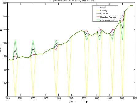
comparison of substitution of missing value for coal
actual missing closet Fit Deviation Approach mean-mode method
19600 1965 1970 1975 1980 1985 1990 1995 2000 2005 2010 500
1000 1500 2000 2500 3000 3500
year
O
il
comparison of substitution of missing value for oil
actual missing closet Fit Deviation Approach mean-mode method
Figure: 2
19600 1965 1970 1975 1980 1985 1990 1995 2000 2005 2010 200
400 600 800 1000 1200 1400 1600
year
na
tur
a
l
gas
comparison of substitution of missing value for Natural gasl
IV. ANALYSISOFALGORITHMCOMPLEXITY:
Step 1 will execute k (no of attribute) times. Time complexity of Step 2 depends on number of object (n), so time complexity is O (n). Time complexity of Step 3 also depends on no of object (n) ,so time complexity is O(n).To identify each missing attribute value we have to check n times .so time complexity for step 4 to step 15 is O(n) ,as all other operation take constant time and ignoring consecutive missing values. so time complexity for step 2 to step 15 is O(n)+O(n)+O(n)=O(n).So the total time complexity of the proposed algorithm is O(k)*O(n)=O(k*n).Also space required to execute the program is constant, so space complexity is O(1). So clearly, computational complexity for proposed algorithm is simple.
V. EXPERIMENTALRESULT
Dataset presented in closet fit [2] has been selected to compare the performance. In Table A an actual dataset is presented. Some attribute values are randomly remove, which are presented in Table B. In Table C we fill up missing attribute values using Closest Fit approach and also present the result if we fill missing values using mean-mode method. In Table D our proposed algorithm has been applied to fill missing attribute values. From table values it is clear that our proposed algorithm can predict better result, compare to mean-mode and best-fit approach. Proposed algorithm can handle consecutive missing values though best-fit approach can’t handle it. In three consecutive figures we compared, these three methods along with actual and missing attribute values considering three attribute separately. From the figure it is clear that not only statistical computation result but also our predicted values are better than other, so our proposed algorithm can be used to generate rule also. So clearly proposed algorithm is easy and efficient to implement in any software packages
VI. CONCLUSIONS
We have to select one method to fill the missing attribute which will give moderately better performance, easy to implement and low cost. In that point of view proposed algorithm may be best for some category of problem where proposed algorithm may be applied. In this work we have discussed application of proposed algorithm on numerical attribute values were missing data are randomly present. We will choose this method (or any statistical based method) to mainly handle missing attribute to take any decision based on statistical data generated from dataset.
VII. REFERENCES
[1] Han, J. and Kamber, M.: “Data Mining: Concepts and Techniques”, Morgan Kaufmann Publishers, 2001.
[2] Gaur, Sanjay and Dulawat, M.S.: “A Closest Fit Approach to Missing Attribute Values in Data Mining”, International
Journal of Advances in Science and Technology, Vol. 2, No.4, 2011.
[3] Pyle, D.: “Data Preparation for Data Mining”. Morgan Kaufmann Publishers, Inc, 1999.
[4] Acock, A.: “Working with Missing Values”. Journal of Marriage and Family, 67,1012-1028. 2005.
[5] Grzymala-Busse, J. W.: “Three Approaches to Missing Attribute Values—A Rough Set Perspective”, Workshop on Foundations of Data Mining, associated with the fourth IEEE International Conference on Data Mining, Brighton, UK, November 1–4, 2004
[6] Young,W., Weckman, G., and Holland, W.: “A survey of methodologies for the treatment of missing values within datasets: limitations and benefits.”, Theoretical Issues in Ergonomics Science Vol. 12, No. 1, 15–43, January– February 2011.
[7] Luengo, J., García,S., Herrera,F., “On the choice of the best imputation methods for missing values considering three groups of classification methods”, Springer-Verlag London Limited 2011.
[8] Zhang,Z., Li, R., Li, Z., Zhang,H., and Yue,G.: “An Incomplete Data Analysis Approach Based on the Rough Set Theory and Divide-and-Conquer Idea”, IEEE,Fourth International Conference on Fuzzy Systems and Knowledge Discovery (FSKD 2007).
[9] Grzymala-Busse, J. W. and Hu,M.: “A Comparison of Several Approaches to Missing Attribute Values in Data Mining”, RSCTC 2000, LNAI 2005, pp. 378−385, 2001,Springer- Verlag Berlin Heidelberg 2001.
[10] Little, R.J.A. and Rubin, D.B., “Statistical Analysis with Missing Data”. New York: John Wiley & Sons, Inc., 1987 [11] Quinlan, J. R., “C4.5: Programs for Machine Learning”.
Morgan Kaufmann Publishers, 1993.
[12] Grzymala-Busse, J. W., and Wang, A. Y., “ Modified algorithms LEM1 and LEM2 for rule induction from data with missing attribute values”. Proc. of the Fifth International Workshop on Rough Sets and Soft Computing (RSSC'97) at the Third Joint Conference on Information Sciences (JCIS'97),Research Triangle Park, , 69– 72, NC, March 2–5, 1997.
[13] Clark, P. Niblett, T.: “The CN2 induction algorithm. Machine Learning 3” , 261–283, 1989.
[14] Knonenko, I., Bratko, and I. Roskar, E.: Experiments in automatic learning of medical diagnostic rules. Technical Report, Jozef Stefan Institute, Lljubljana, Yugoslavia, 1984. [15] Grzymala-Busse, J. W.: “On the unknown attribute values in
[16] Grzymala-Busse, J. W., “Data with missing attribute values: Generalization of indiscernibility relation and rule induction. Transactions on Rough Sets”, Lecture Notes in Computer Science Journal Subline, Springer-Verlag, vol. 1 78–95. 2004
[17] Grzymala-Busse, J. W. “Knowledge acquisition under uncertainty—A rough set approach”. Journal of Intelligent & Robotic Systems 1, 1 , 3–16, 1988
Short Bio Data for the Authors:
Sri. Pallab kumar Dey, MCA, is a faculty of
the Department of Computer Science, The University of Burdwan, West Bengal, India. He has teaching experience of 2 & ½ years. He worked as a Software Developer in Assurgent
Technology Solutions Pvt. Ltd. for 1 year. He is currently working for his PhD degree under Dr. Sripati Mukhopadhyay, Professor Department of Computer Science, The university of Burdwan, in the field Data Mining.