ABSTRACT
TORRES-SAAVEDRA, PEDRO A. Quantile Regression for Repeated Responses Measured with Error. (Under the direction of Drs. Daowen Zhang and Huixia Judy Wang.)
Many problems in biostatistics involve response variables that are difficult to measure ac-curately. Muscular strength in animals and humans quantified through the grip strength, and usual nutrient intake of an individual, are two examples of such variables. These studies of-ten collect, on the same subject, multiple measurements of the response variable containing measurement error. One research interest in these studies is estimating the conditional quan-tile function of the latent response variable given a set of subject-specific covariates and the contaminated replicates.
Conventional quantile regression (QR) is an established technique to estimate the condi-tional quantile function of a response variable. However, it cannot be directly employed for estimation in the current problem because the response variable is observed with measurement error. Naively replacing the latent response variable by the subject-specific average of the con-taminated replicates in a QR model could lead to serious bias in the quantile estimates. Other methods based on transformations have been proposed to estimate the conditional quantiles of a latent variable. However, these methods: i) rely on the existence of a transformation to achieve both constant variance and normality, which could be unrealistic in many problems; and ii) do not provide a method to compute quantile curves when a continuous covariate is present.
Therefore, we propose a new seminonparametric estimation approach to estimate the condi-tional quantile function of a latent variable given subject-specific covariates and contaminated replicates. The proposed method, described in Chapter 2, involves a location-scale shift model that allows the subject-specific random effects to follow a flexible seminonparametric distribu-tion and accounts for measurement errors. A virtue of the proposed method is that it does not rely on the normality and constant variance assumptions on the subject-specific random ef-fects. Moreover, the variance of the subject-specific random effects distribution is allowed to be a function of continuous covariates. We derive the asymptotic results for the proposed estima-tor and, through simulation studies, demonstrate that the proposed method leads to consistent estimates of the conditional quantiles of the latent response variable. To assess the practical usage of the proposed method, a grip strength data set from laboratory mice is analyzed.
usual sodium intake as a function of age. This application entails careful work to deal with the estimation and selection of tuning parameters in our method under a complex survey design. We handle these challenges by incorporating sampling weights into the estimation procedure and a replication method for variance estimation with the proposed method.
Quantile Regression for Repeated Responses Measured with Error
by
Pedro A. Torres-Saavedra
A dissertation submitted to the Graduate Faculty of North Carolina State University
in partial fulfillment of the requirements for the Degree of
Doctor of Philosophy
Statistics
Raleigh, North Carolina 2013
APPROVED BY:
Marie Davidian Leonard Stefanski
Daowen Zhang
Co-chair of Advisory Committee
DEDICATION
To my wife, Marggie this work would not have been possible without your never-failing love, support and encouragement. To my son, Fabian for giving me joy in my life.
A special feeling of gratitude to my loving mother, Aura M., and the rest of my family in Colombia for their support during all these years I have been in school.
BIOGRAPHY
Pedro A. Torres-Saavedra is the son of Pedro L. Torres (deceased), and Aura M. Saavedra. Pedro was born in a small city located in the eastern plains of Colombia. He is the second youngest of ten children, and the only one pursuing a doctoral degree. Pedro graduated in 1996 from a high school located in San Martin, Meta, in the same Colombian region where he was born. He was named the best student in his class. Following his dream of pursuing a professional career, Pedro moved to the capital city, Bogot´a, D.C., to begin his undergraduate studies in Statistics at the National University of Colombia. He was accepted through a program created to recruit outstanding students from low-income families from small municipalities. He finished his undergraduate studies with honors. After graduating he worked as a statistician for a market research company for two years.
Motivated by the desire of acquiring other academic, professional and personal experiences, Pedro left his home country in 2003 to pursue a master degree in Mathematics in Mayag¨uez, Puerto Rico. During his stay in Puerto Rico, Pedro met his wife, Marggie. He then moved to Washington D.C., where he worked for Pacific Institute for Research and Evaluation (PIRE), a non-profit organization. During his tenure in PIRE he provided statistical support for epidemi-ological studies investigating the role of alcohol and drugs in fatal vehicle crashes in the U.S. Pedro was accepted in the Ph.D. program in Statistics at North Carolina State University in 2008. During his stay in North Carolina, his child Fabian was born. Pedro intends to complete his Ph.D. under the direction of Drs. Daowen Zhang and Huixia Judy Wang.
ACKNOWLEDGEMENTS
I would like to thank my advisors Drs. Daowen Zhang and Huixia Judy Wang for their constant support and gentle guidance during this stage of my academic career. I highly appreciate their patience, dedication and willingness to provide feedback in completing this work. Their expertise and achievements have been really inspiring for me. I would like to express my gratitude to Dr. Wang for offering me a research assistantship during my last years in graduate school.
I would like to thank Drs. Marie Davidian, Leonard Stefanski and Michael Sikes for agreeing to serve on my committee. I wish to thank all the faculty and staff at the Department of Statistics at North Carolina State University. This department is a great family that I am proud to belong to. I could not find a better place to build a career as a statistician. I am particularly grateful to Dr. Consuelo Arellano who has always been willing to exchange some words with me about my personal and academic life.
I am also thankful to all my co-workers from GlaxoSmithKline, Drs. Mandy Bergquist, Rick Lewis, David Cooper, Katja Reminger, Steve Novick, and all the researchers I had the opportunity to collaborate with for being such wonderful colleagues and tutors during my experience in the pharmaceutical industry. I would like to thank all the people from PIRE, particularly Drs. Eduardo Romano and Robert Voas who have been mentors and friends. I am also thankful to my former professors from Colombia and Puerto Rico, Drs. David Ospina, Adriana P´erez, Ra´ul Macchiavelli, Edgar Acu˜na and Luis F. C´aceres for being mentors and encouraging me to pursue a doctoral degree.
I want to thank Marggie and Fabian for their patience and understanding during this jour-ney. I am also grateful to my family in Colombia. They are the main reason why I keep dream-ing. I am also thankful to all my friends and classmates who have been incredibly helpful and supportive.
TABLE OF CONTENTS
LIST OF TABLES . . . vii
LIST OF FIGURES . . . ix
Chapter 1 Introduction . . . 1
1.1 Conventional Quantile Regression . . . 4
1.2 Quantile Regression With Measurement Error in Responses . . . 5
Chapter 2 Quantile Regression for Repeated Responses Measured with Error Using a Flexible Distribution . . . 8
2.1 Proposed Method . . . 10
2.1.1 Model Setup . . . 10
2.1.2 Location-Scale Shift Model . . . 11
2.1.3 SemiNonParametric (SNP) Distribution . . . 12
2.1.4 Computational Details . . . 13
2.2 Asymptotic Properties and Inference . . . 15
2.2.1 Resampling Method . . . 17
2.3 Numerical Studies . . . 17
2.3.1 Simulation Design . . . 17
2.3.2 Simulation Results . . . 19
2.4 Application: Conditional Grip Strength Chart for Mice . . . 24
2.5 Conclusions and Discussion . . . 28
Chapter 3 Quantile Curves For Repeated Responses Measured With Error With Application to Usual Sodium Intake . . . 29
3.1 Introduction . . . 29
3.2 Methods . . . 31
3.2.1 Data Description . . . 31
3.2.2 Location-Scale Shift Model . . . 32
3.2.3 B-Splines at a Glance . . . 35
3.3 Computation details . . . 35
3.3.1 Likelihood . . . 35
3.3.2 Tuning Parameters and Starting Values . . . 37
3.3.3 Pointwise Confidence Intervals . . . 38
3.3.4 Balanced Repeated Replication (BRR) . . . 39
3.4 Simulation Study . . . 40
3.4.1 Simulation Design . . . 40
3.4.2 Simulation Results . . . 42
3.5 Quantile Curves of Usual Sodium Intake . . . 46
3.6 Conclusions and Discussion . . . 52
4.1 Introduction . . . 54
4.2 Model Setup . . . 55
4.3 Proposed Methods . . . 56
4.3.1 Corrected-Loss Function . . . 56
4.3.2 Simulation-Extrapolation (SIMEX) . . . 59
4.3.3 Empirical SIMEX . . . 60
4.4 Simulation Studies . . . 61
4.4.1 Simulation Details . . . 61
4.4.2 Simulation Results . . . 62
4.5 Conclusions and Discussion . . . 64
REFERENCES . . . 68
APPENDICES . . . 74
Appendix A . . . 75
A.1 Derivation of Log-Likelihood Function (2.10) . . . 75
A.2 Sketch of the Proof of Theorem 1 . . . 76
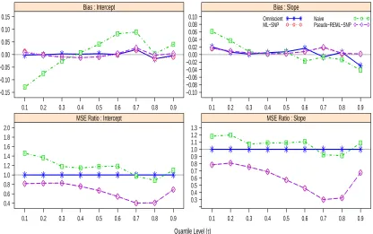
A.3 Simulation Results: Plots of Average Bias and MSE Ratio . . . 80
A.4 Simulation Results: Standard Errors . . . 88
LIST OF TABLES
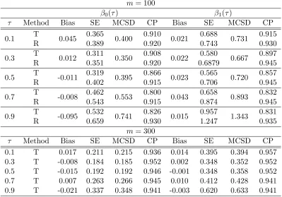
Table 2.1 Standard errors and coverage probabilities for the ML-SNP estimator of quantile coefficients with ui ∼ N(0,1). T: variance estimation method
based on Taylor expansion; R: resampling method; Bias: average bias; MCSD: Monte Carlo standard deviation;SE: average standard error;CP: coverage probability of 95% Wald-type confidence interval. . . 23 Table 2.2 Standard errors and coverage probabilities for the ML-SNP estimator of
quantile coefficients withui ∼0.75N(−1,1) + 0.25N(2,1).T: variance
es-timation method based on Taylor expansion;R: resampling method;Bias: average bias; MCSD: Monte Carlo standard deviation; SE: average stan-dard error; CP: coverage probability of 95% Wald-type confidence interval. 24 Table 2.3 Point estimates (standard errors) of quantile coefficients for mice grip
strength data. The standard errors for the naive estimator were calculated using the Huber’s sandwich method (non-iid option). . . 27 Table 3.1 Distribution of selected number of knots for the naive quantile regression
and ML-SNP method and the selected K for the SNP distribution (tl
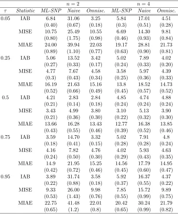
and ts are the number of knots to approximate the location and log-scale functions in the proposed model). . . 42 Table 3.2 Average of integrated absolute bias (IAB×100), mean integrated squared
error (M ISE×100) and mean integrated absolute error (M IAE×100), with its standard error in parentheses: m = 300, ϱ(0.5) = 0.5 and ui ∼ N(0,1). . . 43 Table 3.3 Average of integrated absolute bias (IAB×100), mean integrated squared
error (M ISE×100) and mean integrated absolute error (M IAE×100), with its corresponding standard error in parentheses: m = 300, ϱ(0.5) = 0.50, andui ∼0.75N(−1,1) + 0.25N(2,1). . . 44 Table 4.1 Mean Squared Error (M SE×100) of different estimators of the intercept
β0(τ) and slopeβ1(τ) withui ∼N(0,1). The values in parenthesis are the
standard errors based on 100 replicates. (E)SIMEX-L: (Empirical) SIMEX estimator with linear mean model; (E)SIMEX-Q: (Empirical) SIMEX es-timator with quadratic mean model. CLL: Corrected-loss function based on Laplace measurement errors. CLN: Corrected-loss function based on normal measurement errors. . . 63 Table 4.2 Mean Squared Error (M SE×100) of different estimators of the
Table A.1 Standard errors and coverage probabilities for the ML-SNP estimator of quantile coefficients withui ∼N(0,1),eij ∼N(0,0.25) andn= 4.T:
vari-ance estimation method based on Taylor expansion;R: resampling method; Bias: average bias;MCSD: Monte Carlo standard deviation; SE: average standard error;CP: coverage probability of 95% Wald-type confidence in-terval. . . 88 Table A.2 Standard errors and coverage probabilities for the ML-SNP estimator of
quantile coefficients withui ∼N(0,1), eij ∼N(0,4) and n= 4. T:
vari-ance estimation method based on Taylor expansion;R: resampling method; Bias: average bias;MC SD: Monte Carlo standard deviation;SE: average standard error;CP: coverage probability of 95% Wald-type confidence in-terval. . . 89 Table A.3 Standard errors and coverage probabilities for the ML-SNP estimator of
quantile coefficients withui∼0.75N(−1,1) + 0.25N(2,1),eij ∼N(0,0.25)
and n = 4. T: variance estimation method based on Taylor expansion; R: resampling method; Bias: average bias; MCSD: Monte Carlo standard deviation; SE: average standard error; CP: coverage probability of 95% Wald-type confidence interval. . . 90 Table A.4 Standard errors and coverage probabilities for the ML-SNP estimator of
quantile coefficients with ui ∼ 0.75N(−1,1) + 0.25N(2,1), eij ∼ N(0,4)
and n = 4. T: variance estimation method based on Taylor expansion; R: resampling method; Bias: average bias; MCSD: Monte Carlo standard deviation; SE: average standard error; CP: coverage probability of 95% Wald-type confidence interval. . . 91 Table B.1 Average of mean integrated absolute bias (IAB×100), mean integrated
squared error (M ISE×100) and mean integrated absolute error (M IAE×
100), with its standard error in parentheses: m = 300, ρ(0.5) = 0.75 and
ui ∼N(0,1). . . 92 Table B.2 Average of mean integrated absolute bias (IAB×100), mean integrated
squared error (M ISE×100) and mean integrated absolute error (M IAE×
100), with its standard error in parentheses: m = 300, ρ(0.5) = 0.75, and
LIST OF FIGURES
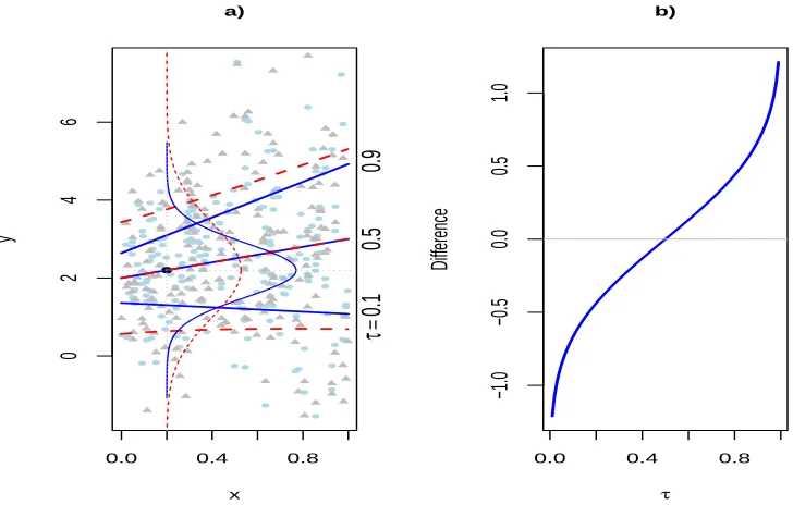
Figure 1.1 a) Conditional quantile lines of Yi∗ at τ = 0.1,0.5 and 0.9 given by
Qτ(Yi∗|xi) (solid) and conditional quantile lines of ¯Yidefined byQτ( ¯Yi|xi)
(dashed). Density functions of Yi∗ (solid) and ¯Yi (dashed) at xi = 0.2. The data points represent the response variable Yi∗ (◦) and ¯Yi (△)
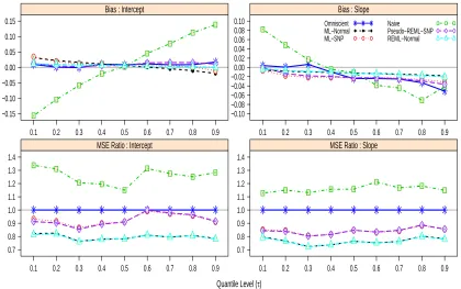
gen-erated from Model (1.4). b) Difference in quantile functions{Qτ( ¯Yi|xi)− Qτ(Yi∗|xi)} atxi = 0.2 as a function of the quantile levelτ. . . 7 Figure 2.1 Average Bias and MSE Ratio of different estimators with respect to the
omniscient estimator of the quantile coefficients with ui ∼N(0,1), m =
100 and n= 4. Reliability ratios: ϱ(0) = 0.50 and ϱ(1) = 0.69. . . 19 Figure 2.2 Average Bias and MSE Ratio of different estimators with respect to the
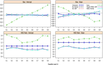
omniscient estimator of the quantile coefficients with ui ∼N(0,1), m =
300 and n= 4. Reliability ratios: ϱ(0) = 0.50 and ϱ(1) = 0.69. . . 20 Figure 2.3 Average Bias and MSE Ratio of different estimators with respect to the
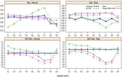
omniscient estimator of the quantile coefficients withui ∼0.75N(−1,1)+
0.25N(2,1), m = 100 and n = 4. Reliability ratios: ϱ(0) = 0.73 and
ϱ(1) = 0.86. . . 21 Figure 2.4 Average Bias and MSE Ratio of different estimators with respect to the
omniscient estimator of the quantile coefficients withui ∼0.75N(−1,1)+ 0.25N(2,1), m = 300 and n = 4. Reliability ratios: ϱ(0) = 0.73 and
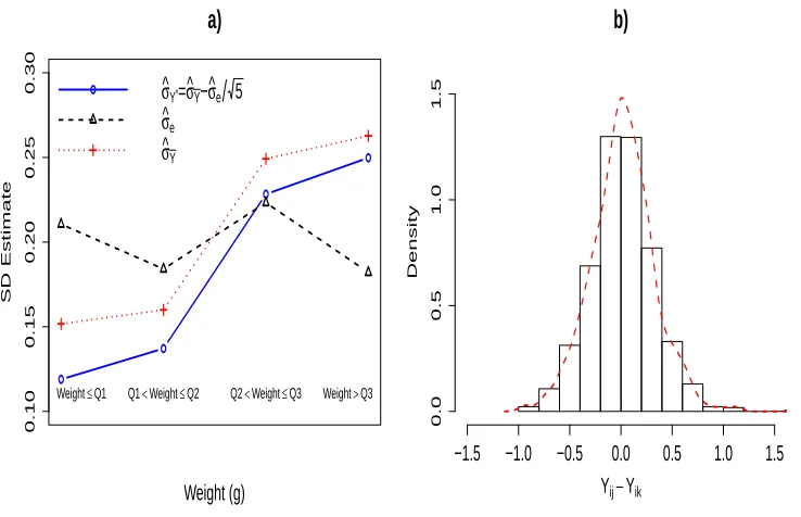
ϱ(1) = 0.86. . . 22 Figure 2.5 a) Method-of-moment estimates of√ √Var(Yi∗) (◦), √Var(ei) (△) and
Var( ¯Yi) (+) based on the model ¯Yi =Yi∗+ ¯ei for four mice subgroups
defined by the quartiles of weight Qr,r = 1,2,3; b) Histogram and ker-nel density estimate (dashed line) of pairwise differences of grip strength measurements: Yij−Yik,i= 1, . . . , m;j, k= 1, . . . ,5. . . 26
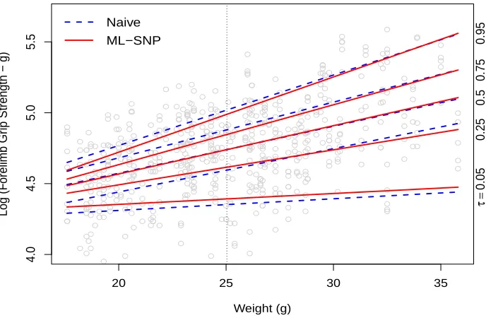
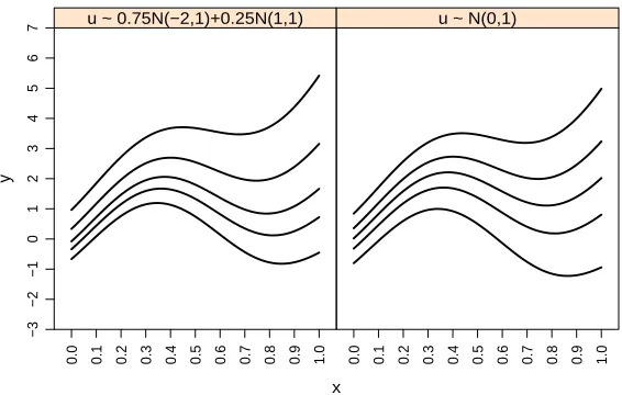
Figure 2.6 Fitted conditional quantile lines in log scale (τ = 0.05,0.25,0.50,0.75,0.95) for mice grip strength data (m = 112). The circles represent the grip strength measurements. The vertical dashed line is the average weight. Some extreme data points were capped to make the graph clearer. . . 27 Figure 3.1 Plot of the true conditional quantile curves for the model used in the
simulation study. The five curves from bottom to top represent τ = 0.05,0.25,0.50,0.75,0.95. . . 41 Figure 3.2 Plot of true (solid), estimated (light dotted), and mean estimated
Figure 3.3 Measurement error diagnostics. Plots of the standard deviation (s.d.) of the log sodium 24HRs vs. the mean of the log sodium 24HRs (column 1). Plots of the s.d. of the log sodium 24 HRs vs. age (column 2). Kernel density estimate of the difference between log sodium 24HRs (dashed), and the density of the normal distribution with mean zero and variance equal to 2ˆσ2e, where ˆσe2 is the estimate of the measurement error variance from the fitted model for each gender (column 3). . . 47 Figure 3.4 Estimated SNP(K= 2) density of log usual sodium usual intake for black
females and black males aged 40. . . 49 Figure 3.5 The estimated quantile curves of usual sodium intake for black females
(m = 839) and black males (m = 839) using naive quantile regression (dashed) and the ML-SNP(K = 2) (solid) methods. For each method, the five curves from bottom to top for each method represent τ = 0.05, 0.10, 0.25, 0.50, 0.75, 0.90. The horizontal lines at 1500 mg and 2300 mg represent the recommended adequate intake level and tolerable upper intake limit. Filled circles represent the average of sodium 24HRs. . . 50 Figure 3.6 Median (τ = 0.50) usual sodium intake and 95% pointwise confidence
intervals for black females and black males using a SNP(K= 2) distribu-tion. The horizontal lines at 1500 mg and 2300 mg show the recommended adequate intake level and tolerable upper intake limit. The bands repre-sent the 95% pointwise confidence intervals calculated using the BRR method. . . 51 Figure 3.7 Percentage of individuals with usual sodium intake below the
recom-mended adequate intake level (1500 mg), and tolerable upper intake level (2300 mg) using the naive quantile regression and ML-SNP(K= 2) meth-ods. . . 52 Figure 4.1 Bias of different estimators of the intercept β0(τ) and slope β1(τ) at
τ = 0.50,0.75 and 0.90 for model with ui ∼N(0,1). (E)SIMEX-L: (Em-pirical) SIMEX estimator with linear mean model; (E)SIMEX-Q: (Empir-ical) SIMEX estimator with quadratic mean model. CLL: Corrected-loss function based on Laplace measurement errors and normal kernel smooth-ing. CLN: Corrected-loss function based on normal measurement errors and sine integral smoothing. . . 65 Figure 4.2 Bias of different estimators of the intercept β0(τ) and slope β1(τ) at
τ = 0.50,0.75 and 0.90 for model with ui ∼ χ23. (E)SIMEX-L:
Figure A.1 Average Bias and MSE Ratio of different estimators with respect to the omniscient estimator of the quantile coefficients with ui ∼N(0,1), eij ∼ N(0,0.25),m= 100 andn= 4. Reliability ratios:ρ(0) = 0.80 andρ(1) = 0.90. . . 80 Figure A.2 Average Bias and MSE Ratio of different estimators with respect to the
omniscient estimator of the quantile coefficients with ui ∼N(0,1), eij ∼ N(0,0.25),m= 300 andn= 4. Reliability ratios:ρ(0) = 0.80 andρ(1) = 0.90. . . 81 Figure A.3 Average Bias and MSE Ratio of different estimators with respect to the
omniscient estimator of the quantile coefficients with ui ∼N(0,1), eij ∼ N(0,4),m= 100 andn= 4. Reliability ratios:ρ(0) = 0.20 andρ(1) = 0.36. 82 Figure A.4 Average Bias and MSE Ratio of different estimators with respect to the
omniscient estimator of the quantile coefficients with ui ∼N(0,1), eij ∼ N(0,4),m= 300 andn= 4. Reliability ratios:ρ(0) = 0.20 andρ(1) = 0.36. 83 Figure A.5 Average Bias and MSE Ratio of different estimators with respect to the
omniscient estimator of the quantile coefficients withui ∼0.75N(−1,1)+ 0.25N(2,1), eij ∼ N(0,0.25), m = 100 and n = 4. Reliability ratios: ρ(0) = 0.91 and ρ(1) = 0.96. . . 84 Figure A.6 Average Bias and MSE Ratio of different estimators with respect to the
omniscient estimator of the quantile coefficients withui ∼0.75N(−1,1)+
0.25N(2,1), eij ∼ N(0,0.25), m = 300 and n = 4 subjects. Reliability ratios: ρ(0) = 0.91 andρ(1) = 0.96. . . 85 Figure A.7 Average Bias and MSE Ratio of different estimators with respect to the
omniscient estimator of the quantile coefficients withui ∼0.75N(−1,1)+ 0.25N(2,1), eij ∼N(0,4), m = 100 and and n= 4 subjects. Reliability ratios: ρ(0) = 0.40 andρ(1) = 0.60. . . 86 Figure A.8 Average Bias and MSE Ratio of different estimators with respect to the
omniscient estimator of the quantile coefficients withui ∼0.75N(−1,1)+ 0.25N(2,1), eij ∼N(0,4), m= 300 and n= 4. Reliability ratios: ρ(0) =
Chapter 1
Introduction
Many problems in biostatistics involve response variables that are either unobservable or difficult to measure. Muscular strength in animals and humans quantified through the grip strength is an example of such a variable. Multiple measurements of grip strength, which contain considerable measurement error, are usually taken on the same subject. One research interest in grip strength studies is to construct conditional charts based on a set of conditional quantiles of the latent grip strength, given the contaminated replicates and covariates information. Another typical example of a latent response variable is usual nutrient intake, which is defined as the long-term average of the daily nutrient intake by an individual. Typically, a small number of 24-hour food recalls are collected to make inferences on the conditional distribution of usual nutrient intake. These 24-hour recalls contain substantial measurement errors, which arise from different sources. Estimating conditional quantiles of usual nutrient intake is a crucial task for designing and implementing dietary guidelines and policies. These applications will be revisited in Chapters 2 and 3, respectively.
To introduce our research problem, we let Yi∗ and Yij be the latent response variable and
the contaminated replicatejfor the individuali(i= 1, . . . , m;j= 1, . . . , ni), respectively. The
p-dimensional vector of subject-specific covariates is denoted by xi. In the previous motivating examples, the inference target is the conditional quantile function ofYi∗ given a set of subject-specific covariatesxi, denoted by Qτ(Yi∗|xi), where 0< τ <1 is the quantile level.
To estimate quantiles of a latent variable when contaminated replicates are available, some authors have proposed estimation methods based on additive measurement errors following a normal distribution. These methods do not include information about subject-specific covariates
(Cook and Stefanski, 1994). Delaigle et al. (2008) suggested estimating the distribution of Yi∗
using nonparametric deconvolution.
When the inference target is the estimation of the conditional quantile functionQτ(Yi∗|xi), a
tool that comes to mind is conventional quantile regression (Koenker, 2005). However, since the response variable in the current problem is observed with measurement error, quantile regression cannot be directly used. A tempting strategy to overcome this problem would be employing the subject-specific average of the contaminated replicates{Yij}, namely ¯Yi=n−i 1
∑ni
j=1Yij, as the
response variable in a conventional quantile regression model (Variyam, 2003; Barreiro et al., 2010; Molenaar et al., 2010). Nonetheless, naively replacingYi∗ by ¯Yi to estimateQτ(Yi∗|xi) will
generally lead to seriously biased estimates ofQτ(Yi∗|xi) as a consequence of the measurement error present in ¯Yi. The bias in the estimate of the conditional quantile function depends, among other factors, on the magnitude of the measurement errors and the quantile levels of interest. The presence of large measurement errors and tail quantiles are favorable conditions for obtaining large bias in the quantile estimates. This problem is discussed in more detail in Section 1.2.
Unlike the measurement error in the response variable, estimation methods for quantile regression with mismeasured covariates has captured more attention in the literature. Schen-nach (2008) proposed a method for quantile regression with mismeasured covariates based on instrumental variables. Wei and Carroll (2009) considered the estimation of linear conditional quantiles in the presence of covariate measurement error. Some limitations of their method is that it assumes that the whole quantile process of the latent variable is a linear function of covariates, and it is computationally intensive.
Other methods based on transformations have been proposed to estimate conditional quan-tiles of a latent variable when responses are measured with error. Tooze et al. (2010) proposed fitting a classical linear mixed model after applying a Box-Cox transformation to the observed 24-hour recalls. The conditional quantiles of usual nutrient intake are estimated using an ap-proximation formula for usual nutrient intake and Monte Carlo simulation. Some caveats of the transformation-based methods are: i) they rely on the existence of a transformation to achieve both constant variance and normality, which could be unrealistic in many problems; and ii) they do not provide a method to compute conditional quantile curves when a continuous co-variate is present. For instance, if the variable age is included in the model then estimates of the conditional quantiles of usual nutrient intake for age intervals are delivered instead.
the contaminated replicates such that the measurement errors are additive and follow a normal distribution with constant variance. However, our method does not assume constant variance and normality for the specific random effects. Moreover, the variance for the subject-specific random effects is allowed to be a function of continuous covariates. This feature enables the construction of conditional quantile curves of the latent response variable under the presence of continuous covariates, a limitation of the existing methods based on data transformations. The proposed method is presented in Chapter 2. We derive the asymptotic properties of the proposed estimator and, through simulation studies, demonstrate that the proposed method leads to consistent estimates of the conditional quantiles of the latent response variable. To assess the practical usage of the proposed method, a grip strength data set from laboratory mice is analyzed.
To allow more flexibility in the proposed method, we extend the location-scale shift model proposed in Chapter 2 by allowing the location and scale functions to be modeled nonpara-metrically. This current model, introduced in Chapter 3, handles the possible misspecification of the location and scale functions in the model proposed in Chapter 2. Empirical evidence suggests that the proposed estimator in Chapter 3 outperforms the naive estimator that as-sumes a nonparametric quantile regression model with ¯Yi as the response variable and B-spline basis functions to approximate the quantile curves. In order to illustrate its value, we apply the proposed method to estimate conditional quantile curves of usual sodium intake as a function of age. In this application, inferential aspects of complex survey designs (i.e., weighting and variance estimation) are incorporated into the estimation process of the proposed method.
1.1
Conventional Quantile Regression
Conventional quantile regression, originally introduced by Koenker and Bassett (1978), is a regression technique that examines the influence of covariates on the tails of the response dis-tribution. Quantile regression complements the traditional mean regression models by allowing analysts to model not only the mean that measures the center, but also tail quantiles of the conditional distribution of the response variable as functions of a set of covariates. An appeal-ing feature of quantile regression is that it does not assume a parametric form of the error distribution in the regression model.
There exists a vast literature about quantile regression and its applications when the re-sponse variable is observed without measurement error (Koenker, 2005; Wang and Fygenson, 2009; Wang and Zhou, 2010). We briefly introduce the quantile regression estimator in the context of a linear model. Let us assume that the response variableYi∗ has been observed, and that the conditional quantile function of Yi∗ is linear inxi, namely
Qτ(Yi∗|xi) =xTi β0(τ), (1.1) where β0(τ) is the true quantile coefficient. The quantile coefficients β0(τ) in (1.1) can be
estimated for any τ ∈(0,1) by
ˆ
β(τ) = min
β∈Rp
m ∑
i=1
ρτ(Yi∗−xTi β), (1.2)
whereρ(ϵ) =ϵ{τ−I(ϵ <0)}, andI(·) is the indicator function (Koenker, 2005). The estimator ˆ
β(τ) also satisfies that
m−1/2 m ∑
i=1
ψτ{Yi∗,xi,βˆ(τ)}=op(1), (1.3)
where ψτ(Yi∗,xi,βˆ) = xi{I(Yi∗ −xTiβˆ < 0)−τ}. Note that E[ψτ{Yi∗,xi,β0(τ)}] = 0 when
Model (1.1) holds. Therefore,ψτ(Yi∗,xi,β) is an unbiased estimating function forβ0(τ).
Problem (1.2) can be solved using linear programming techniques such as the simplex al-gorithm, or interior point methods (Koenker, 2005). In the following result it is assumed that the regression errors haveτth quantile equal to zero for the intercept inβ(τ) to be identifiable. Under some regularity conditions and assuming a linear model with independent and identi-cally distributed errors, Koenker (2005) showed that√m{βˆm(τ)−β0(τ)}converges to a normal
distribution with zero mean and asymptotic covariance matrix given by ω2D−01, where
D0 = lim
m→∞m
−1∑
i
ω =τ(1−τ)/f(0) and f(0) is the density function of the regression errors evaluated at zero. The term 1/f(0) is called the sparsity function (Koenker, 2005). Note that the asymptotic variance of the quantile estimator at a givenτ is large whenf(0) is small. Directly estimating the asymptotic covariance matrix of ˆβ(τ) is challenging as it requires estimating the unknown sparsity function. Therefore, some authors have proposed estimating the asymptotic standard errors of ˆβ(τ) by using resampling methods such as bootstrap (Horowitz, 1998; Jin et al., 2001). Quantile functions enjoy an important property called equivariance to monotone transfor-mations (Koenker, 2005, p. 39). This property is not shared by the mean function. Specifically, if
h(·) is a monotone transformation then Qτ{h(Yi∗)|xi}=h{Qτ(Yi∗|xi)}. For the mean function E{h(Yi∗)|xi} ̸=h{E(Yi∗)|xi}, except in very special cases (e.g., whenhis linear). This property of the quantile functions facilitates the estimation of quantiles after data transformations. The mean function, however, enjoys linearity, a property not shared by the quantile function, except in some very particular situations, such as comonotonic random variables (Koenker, 2005). The equivariance property of the quantile functions plays an important role in the proposed meth-ods given the customary practice of transforming the data to achieve the classical measurement error assumptions. These aspects related to data transformations in quantile estimation will be revisited in Chapters 2 and 3.
Another issue in quantile regression is crossing quantiles. Quantile functions must satisfy that Qτ1(Yi∗|xi) ≤Qτ2(Yi∗|xi), whenever τ1 ≤τ2. This fact is the result of the nondecreasing
property of distribution functions. In finite samples, however, estimates of Qτ(Yi∗|xi) for two
quantile levels close to each other may violate the nondecreasing property, that is, the lower quantile may be estimated larger than the higher quantile. Some strategies to avoid the crossing quantile issue have been proposed in literature (He, 1997; Bondell et al., 2010).
Readers interested in other topics of quantile regression can refer to Koenker (2005) and references therein. In his monograph, Koenker (2005) provides an excellent review of the theory and applications of quantile regression. Many of the methodological developments presented in his monograph as well as more recent developments in quantile regression topics have been already implemented in theRlibraryquantreg (Koenker, 2012). Commercial software packages, such as SAS, also includes procedures (e.g., proc quantreg) to fit quantile regression models under different scenarios (SAS 9.3, 2012).
1.2
Quantile Regression With Measurement Error in Responses
subject-specific average ¯Yi = n−i 1 ∑ni
j=1Yij as the response in a linear regression model with
subject-specific covariates. Buonaccorsi (1996) and Carroll et al. (2006) provided a detailed discussion about the problem of measurement error in the response in mean regression models. However, if we change the inference target from the conditional mean E(Yi∗|xi) to the
condi-tional quantile function Qτ(Yi∗|xi) for a given τ, replacing Yi∗ by ¯Yi could lead to misleading conclusions about the conditional quantiles of Yi∗. To illustrate this point, let us consider the following location-scale shift model
Yij =Yi∗+eij = 2 +xi+ (0.5 +xi)ui+eij, (1.4) wherexi ∼U(0,1), ui ∼N(0,1), eij ∼N(0, σ2e = 2), andui and eij are independent one from
the other. Under Model (1.4) it is clear that E(Yi∗|xi) = E( ¯Yi|xi). The conditional quantile function of Yi∗ is equal toQτ(Yi∗|xi) =β0(τ) +β1(τ), where β0(τ) = 2 + 0.5Φ−1(τ), β1(τ) =
1+Φ−1(τ), and Φ−1(·) is the inverse cumulative distribution function ofN(0,1). The conditional quantile function of ¯Yi is equal to
Qτ( ¯Yi|xi) = 2 +xi+ Φ−1(τ) √
(0.5 +xi)2+σe2/ni,
which is a non-linear function ofxi. Moreover, Qτ(Yi∗|xi)≠ Qτ( ¯Yi|xi) for allτ ̸= 0.5.
These issues with the naive approach are further illustrated in Figure 1.1. The part a) of this figure plots the data points generated using Model (1.4) withm = 200 individuals andni = 2
contaminated replicates for each individual. The true conditional quantile lines ofYi∗and ¯Yifor
τ = 0.1,0.5 and 0.9 are illustrated in Figure 1.1. The conditional median lines are the same. In this particular case, naively replacingYi∗by ¯Yiin a conventional quantile regression model leads
to unbiased estimates ofQ0.5(Yi∗|xi) becauseQ0.5(Yi∗|xi) =Q0.5( ¯Yi|xi) = 2 +xi. However, if the inference target are tail quantiles such asτ = 0.1 or 0.9, naive estimates can be seriously biased. Naive quantile regression tends to underestimate lower quantiles, whereas it overestimates upper quantiles. Furthermore, naive quantile regression assumes a linear conditional quantile function for ¯Yi, regardless the fact thatQτ( ¯Yi|xi) is a non-linear function ofxi. In other words, the naive
method suffers from model misspecification. Part a) of Figure 1.1 also plots the conditional density function ofYi∗ and ¯Yi atxi = 0.2. The density function of ¯Yi shows a larger dispersion around the conditional mean as a consequence of the measurement error. In fact, using Model (1.4) we have that Var( ¯Yi|xi) = (0.5 +xi)2+σe2/2>Var(Yi∗|xi) = (0.5 +xi)2 when σe2>0.
On the other hand, the part b) in Figure 1.1 illustrates the difference between the quantile functions, namely{Qτ( ¯Yi|xi)−Qτ(Yi∗|xi)}, atxi= 0.2 as a function of the quantile levelτ. From
0.0 0.4 0.8
0
2
4
6
a)
x
y
τ=
0.1
0.5
0.9
0.0 0.4 0.8
−1.0
−0.5
0.0
0.5
1.0
b)
τ
Diff
erence
Figure 1.1: a) Conditional quantile lines ofYi∗atτ = 0.1,0.5 and 0.9 given byQτ(Yi∗|xi) (solid) and conditional quantile lines of ¯Yidefined byQτ( ¯Yi|xi) (dashed). Density functions ofYi∗(solid)
and ¯Yi (dashed) at xi = 0.2. The data points represent the response variable Yi∗ (◦) and ¯Yi
(△) generated from Model (1.4). b) Difference in quantile functions {Qτ( ¯Yi|xi)−Qτ(Yi∗|xi)} atxi = 0.2 as a function of the quantile levelτ.
also larger at tail quantiles. Based on the previous discussion, it is clear that using conventional quantile regression with ¯Yi as the response variable is in general not appropriate to estimate
Chapter 2
Quantile Regression for Repeated
Responses Measured with Error
Using a Flexible Distribution
Some problems in medicine and biology are characterized by the presence of a response variable
Yi∗ that is difficult to measure accurately. Usual nutrient intake (Variyam, 2003; Dodd et al., 2006; Tooze et al., 2010), blood pressure (Jackson et al., 2007), grip strength (Gunther et al., 2008; Barreiro et al., 2010; Molenaar et al., 2010; Wind et al., 2010) and pulmonary function (Kulich et al., 2005) are some examples of such variables. In order to make inferences on the conditional distribution ofYi∗, several repeated measurements or contaminated replicates ofYi∗, sayYij, are often taken on the same subject with errors. The number of contaminated replicates
is typically between 2 and 5 because of the high cost, effort and time involved.
Our research is in part motivated by the construction of conditional grip strength charts for laboratory mice. Conditional reference charts can help monitor growth, follow progress after treatment and identify abnormal cases. Reference charts for a latent variable are more broadly applicable than those based on subject-specific averages of the repeated measurements, since the latter are lab-specific, depending on the experimental protocols (e.g., repetition of measurements, dynamometers used, muscle relaxation time, etc). From a statistical point of view, our aim is to estimate the conditional quantile function of the unobserved variable Yi∗
given covariates information xi, denoted by Qτ(Yi∗|xi), 0 < τ < 1, using the contaminated
replicates {Yij}. The estimation of Qτ(Yi∗|xi) is driven by the interest of characterizing the
conditional quantile function instead of the mean function ofYi∗ givenxi.
Researchers from different fields often use conventional linear quantile regression (QR) with the subject-specific average of the repeated measurements as the response variable to estimate
suf-fers from model misspecification and often leads to biased estimates of the conditional quantiles of the latent response as well as the covariate effects on the latent response.
In the measurement error literature, researchers have discussed the estimation of quantiles of a latent variable when no covariates are present. In the context of parametric deconvolution and classical measurement error problem, Carroll et al. (2006) proposed modeling the latent variable with a flexible distribution. Schechtman and Spiegelman (2007) proposed two esti-mation methods, Simulation-Extrapolation (SIMEX) (Cook and Stefanski, 1994) and efficient bootstrap combined with Jackknife. Li and Vuong (1998) used the empirical characteristic func-tion of pairs of repeated measurements to derive nonparametric estimators of the density of a latent variable. Delaigle et al. (2008) suggested two deconvolution estimators for the density function of an unobserved variable based on contaminated replicates.
More recently, Tooze et al. (2010) discussed the estimation of conditional quantiles of Yi∗
when covariates are present. They proposed a linear mixed effects model with normal random effects after applying a Box-Cox transformation to the replications of nutrient intake{Yij}. The conditional quantiles ofYi∗ are estimated via Monte Carlo replication and Taylor linearization. Although they showed that their method performs well empirically, it has some drawbacks. First, in more general contexts a Box-Cox transformation may not reach constant variance and normality in both the measurement errors and the subject-specific random effects (Eckert et al., 1997; Fitzmaurice et al., 2007). Consequently, a classical linear mixed model could lead to biased estimates of the conditional quantiles of the latent response. Second, their method pro-duces point estimates of the conditional quantiles for groups defined by categorizing continuous covariates. That is, quantile curves as a function of continuous covariates cannot be accommo-dated in this method. Third, the interpretation of the effect of covariates on the conditional distribution of the latent response is obscured after applying a non-trivial transformation to the data.
Therefore, we propose a seminonparametric method to estimate the conditional quantile function of a latent variable in a regression setting. We consider a two-stage model involving a regression model with heteroscedastic errors for the latent variable and the measurement error process. We allow the regression errors in the model for the latent variable to follow a flexible distribution. These features of the proposed model overcome some of the limitations of the existing methods that assume constant variance and normality after transforming the data.
2.1
Proposed Method
2.1.1 Model Setup
Let Yi∗ be a latent response variable and xi a p×1 vector of covariates for the ith subject,
i= 1, . . . , m. Throughout, we assume that the first element of xi is one corresponding to the intercept. For a given subject, the covariates inxi, for instance, gender or weight, are assumed
to remain constant across the repeated measurements. Our main objective is to estimate the conditional quantile function of the latent variableYi∗ givenxi, defined asQτ(Yi∗|xi) = inf{t∈
R:P(Yi∗≤t|xi)≥τ}, where 0< τ <1 is the quantile level. To this objective, we assume that Yi∗ and xi are related through the following model
Yi∗ =f(xi,β) +σ(xi,γ)ui, (2.1)
where f(·) and σ(·) are known location and scale functions, respectively, β and γ are un-known parameter vectors, and ui are the regression errors that follow a flexible seminon-parametric (SNP) distribution. The function f(xi,β) corresponds to the mean function when
E(ui) = 0, while σ2(xi,γ) is the variance function when Var(ui) = 1, and it represents the heteroscedasticity in the data. To capture heteroscedasticity, two scale functions are commonly used, σ(xi,γ) = xTi γ and σ(xi,γ) = exp(xTi γ) (Davidian and Carroll, 1987). The former
case leads to a location-scale shift model (Koenker, 2005; Wang and Fygenson, 2009). Other proposals for variance functions can be found in Davidian and Carroll (1987).
Model (2.1) allows heteroscedastic errors, which can be found in many applications. For instance, Barreiro et al. (2010) computed reference values of respiratory and peripheral muscle function in laboratory rats. Their results suggest that the forelimb grip strength variance in-creases with rats’ weight. In another work in healthy Caucasian adults, Gunther et al. (2008) showed that the grip strength variance tends to decrease with patients’ age.
To allow more flexibility in Model (2.1) we assume that the true density of the regression errorsui belongs to a class of smooth densities having a continuous and strictly increasing
Under Model (2.1) the conditional quantile function ofYi∗ takes the following form
Qτ(Yi∗|xi) =f(xi,β) +σ(xi,γ)HK−1(τ,a), (2.2) whereHK−1(τ,a) represents the quantile function ofui. This quantile function can take different
forms depending on the functional forms of the location and scale functions, and the parameters of the SNP distribution.
2.1.2 Location-Scale Shift Model
A particular case of Model (2.1) is the location-scale shift model
Yi∗ =xTi β+ (xTi γ)ui, (2.3)
where β and γ are p-dimensional unknown vectors. In Model (2.3) the covariates affect both the location and scale of the conditional distribution of Yi∗ given xi, but they have no effect
on the basic shape of the distribution that is dictated byHK(ui,a). The conditional quantile function resulting from Model (2.3) is
Qτ(Yi∗|xi) =xTi β(τ) =xTi {β+γHK−1(τ,a)}, (2.4)
provided that xTi γ > 0 in the domain of xi. Although the location-scale shift Model (2.3) assumes the conditional quantiles ofYi∗ are linear inxi, this model is convenient and has been
widely used in quantile regression settings (Koenker and Bassett, 1978; He, 1997; Reich et al., 2010; Wang and Zhou, 2010). All the developments in the remaining sections make reference to this particular model, though the proposed method can be extended to more general models.
IfYi∗ were observed, the quantile coefficientsβ(τ) in (2.4) can be estimated by the conven-tional quantile regression estimator
ˆ
β(τ) = arg min
β∈Rp
m ∑
i=1
ρτ(Yi∗−xTi β), (2.5)
where ρτ(ϵ) = ϵ{τ −I(ϵ < 0)} is the check function (Koenker, 2005), and I(·) denotes the
indicator function. However, in some applicationsYi∗ is difficult to measure accurately. Instead, a small numberni of contaminated replicates{Yij}ni
j=1 are taken on the same subjecti. For the
observed response variableYij, we assume the classical measurement error model
Yij =Yi∗+eij, (2.6)
(Car-roll et al., 2006), and the parameter σe2 is the measurement error variance. The model for the observed response according to (2.3) is then given by
Yij =xTiβ+ (xiTγ)ui+eij. (2.7)
Model (2.7) differs from the classical linear mixed model since the former includes a single term for the random effectsui that could follow non-normal distributions, and its design matrix for the random effects includes the unknown parameterγ. As a consequence, the existing software for LMMs cannot be directly used to obtain estimates for Model (2.7).
In the naive approach, Qτ(Yi∗|xi) is estimated by using a linear quantile regression model with ¯Yi =n−1
∑n
j=1Yij as the response variable. The naive approach, which assumes linearity
of quantile functions, suffers from model misspecification under Model (2.7). Therefore, it may lead to serious bias in the conditional quantile estimates ofYi∗. This issue is discussed in detail in Section 1.2.
2.1.3 SemiNonParametric (SNP) Distribution
In the proposed method we assume that the subject-specific random effectsui follows an SNP distribution with density belonging to a class of smooth densities, introduced originally in the econometrics context (Gallant and Nychka, 1987; Davidian and Gallant, 1993). In general, ui
can be written as ui = µ+σZi, where µ and σ are the location and scale parameters of the subject-specific random effects distribution and Zi follows a standard SNP distribution.
Henceforth we letui=Zi to avoid an overparameterized model. A univariate random variable
Z follows a standard SNP distribution if its density is given by
hK(z,a) =PK2(z,a)ϕ(z) = (aTz)2ϕ(z), (2.8)
where z = (1, z,· · ·, zK)T, K is the degree of the polynomial PK(·), a = (a0, a1,· · · , aK)T comprises the (K + 1) polynomial coefficients and ϕ(z) is the standard normal density. As an example, if K = 2 then P2(z) = a0 +a1z+a2z2. When K = 0 the function hK(z,a)
becomes the density of the standard normal distribution. In the definition (2.8) the normal density can be substituted by any other density having a moment generating function (Gallant and Nychka, 1987). The SNP family includes skewed, leptokurtic, platykurtic, or multi-modal densities (Davidian and Giltinan, 1995). A comprehensive discussion of the SNP estimator and its properties can be found in Gallant and Nychka (1987); Davidian and Gallant (1993); Fenton and Gallant (1996a,b); Kim (2007) and Takada (2008). The use of the SNP distribution as a parametric family is discussed in Le´on et al. (2009).
authors have proposed alternative methods mainly in the context of linear mixed models. Some approaches are the smooth nonparametric maximum likelihood estimator (Magder, Laurence and Zeger, 1996), heterogeneity model (Verbeke and Lesaffre, 1996), smoothing by roughening (Shen and Louis, 1999), and penalized Gaussian mixture (Ghidey et al., 2004, 2010). Nonethe-less, we adopt the SNP distribution because it is flexible, and the resulting likelihood function has a closed form, which makes the computation more straightforward.
2.1.4 Computational Details
Likelihood
Let Yi = (Yi1, . . . , Yini)
T be the n
i-dimensional column vector of repeated measurements for
theith subject. The location-scale shift model (2.7) can be written as
Yi =Xiβ+ (Xiγ)Zi+ei, (2.9)
where Xi = 1ni ⊗x
T
i is a (ni ×p) design matrix, 1ni is a ni-dimensional column vector of
ones and⊗ denotes the usual Kronecker product,Zi is a univariate random variable following a standard SNP distribution andei is a ni×1 vector that comprises the measurement errors
associated with theith subject. In our implementation we assume thatei ∼N(0, σe2Ini), where
Ini is the identity matrix of orderni, but the proposed method can be extended to models with
other measurement error distributions.
In Model (2.9) the parameter vector of dimension d = 2p + K + 1 is given by θ = (βT,γT,φT, σ2
e)T, where the K-dimensional vector φ results from the reparameterization of
the polynomial coefficients a introduced in Section 2.1.3. This reparameterization allows one to use unconstrained optimization techniques to compute the MLE of θ (Zhang and David-ian, 2001; Chen et al., 2002). The suggested reparameterization is described as follows. Define
A= E(U UT), where U = (1, U,· · · , UK)T and U ∼N(0,1). The matrixA is required to sat-isfy the constraintE[PK2(U,a)] =aTAa= 1, which guarantees that hK(u,a) is truly a density function. Since A is positive definitive then A=BTB, whereB is a positive definite matrix.
Now, consider the following polar coordinate transformation that maps the vector a ∈ RK+1
into φ ∈ RK, −π/2 < φi ≤ π/2, i = 1, . . . , K. Let c = Ba, where the elements of c are defined as: c1 = sin(φ1), cj = sin(φj)
∏j−1
l=1 cos(φl), j = 2, . . . , K, and cK+1 = ∏K
l=1cos(φl).
The original polynomial coefficients can be computed as a=B−1c. The log-likelihood function based on Model (2.9) can be written as
ℓ(θ;Y) =
m ∑
i=1 [
logp(Yi;θ) + logEZi|Yi;θ
{
PK2(Zi) }]
wherep(Yi;θ) is the normal density with mean and variance
E(Yi;θ) =Xiβ, Var(Yi;θ) =σ2eIni + (x
T
i γ)2Jni, (2.11)
Ini is the identity matrix of order ni and Jni is the square matrix of ones of dimension ni.
GivenYi, the random variable Zi in (2.10) has a normal density with mean
E(Zi|Yi;θ) ={ni(xTi γ)( ¯Yi−xTi β)}/{σe2+ni(xTi γ)2}, (2.12) and variance
Var(Zi|Yi;θ) =σe2/{σ2e+ni(xTi γ)2}. (2.13) The matrix Var(Yi;θ) in (2.11) resembles a covariance matrix having a compound symmetry
structure resulting from the classical linear model with random intercepts, namelyYi=Xiβ+
1nibi+eiwithbi∼N(0, σ
2
b). However, the variance of the random effects in the latter modelσb2
has been substituted by the term (xTi γ)2 in (2.11). The derivation of the log-likelihood (2.10) is presented in Appendix A.1.
MLE and REML
The log-likelihood (2.10) involves a normal-based likelihood and higher moments of a normal distribution that have closed forms. Therefore, the function (2.10) can be maximized using standard optimization algorithms such as Quasi-Newton Rapshon. For the particular case of
K = 0 (corresponding to a normal distribution), Restricted Maximum Likelihood (REML) estimates for θ may be obtained as well (Harville, 1977). Unlike the normal case, the REML function is not readily available whenK ≥1. Nonetheless, we mimic the normal-based REML by subtracting the term 12log∑mi=1XT
i Vi−1Xi from the log-likelihood function defined by
(2.10), where | · | denotes its determinant and Vi = Var(Yi|xi) under Model (2.9) with SNP
random effects, i.e.,Vi=σe2Ini+Var(Zi)(x
T
i γ)2Jni. We call this approach pseudo-REML based
on an SNP distribution. Its inclusion, like the REML, aims to reduce the bias in estimating variance components when the sample size is small to moderate.
the optimization routine if the location-scale shift model provides a reasonable fit to the data. Moreover, as suggested by He (1997), negative values ofxTi γ resulting from the unconstrained optimization may be an indication of model misspecification.
Selection of K
The polynomial degreeKinhK(z,a) can be selected by using adaptive rules such as the Schwarz
criterion (BIC), Akaike criterion (AIC) or Hannan-Quinn (HQ) criterion (Hannan, 1987). In our numerical studies we use the HQ criterion to select K for the SNP distribution. This criterion has been advocated by Davidian and Gallant (1993) as an automatic selection rule forK. The HQ criterion has shown to perform well in problems involving Hermite series expansions as in the definition of the SNP estimator (Davidian and Gallant, 1993). The HQ criterion is defined as −l( ˆθ;Y) +dlog(logN), where d is the dimension of θ and N = ∑mi=1ni. The parameter K plays the role of a tuning parameter. In many applications values of K = 0,1,2 may be enough to approximate the true distribution of interest (Davidian and Gallant, 1993; Zhang and Davidian, 2001; Chen et al., 2002). For highly skewed distributions, though, larger values of K are needed in order to get a better approximation (Fenton and Gallant, 1996a,b; Kim, 2007; Takada, 2008).
2.2
Asymptotic Properties and Inference
The conditional quantile function of Yi∗ can be estimated by ˆQτ(Yi∗|xi) = xTi βˆ(τ), where
ˆ
β(τ) = ˆβ+ ˆγHK−1(τ; ˆφ). For a given τ and ˆφ, the quantityHK−1(τ; ˆφ) can be found by solving the nonlinear equationHK(z; ˆφ) =τ forz. In our implementation we used the bisection method to compute the quantiles of the SNP distribution.
The asymptotic properties of the ML-SNP estimator ˆβ(τ) are discussed in Theorem 1. In developing the proposed method we assume a typical repeated measurements scenario where the number of repeated measurements ni are bounded and the number of subjects m → ∞
(Demidenko, 2004; Wang and Fygenson, 2009).
Theorem 1 Letθ0 be the true parameter vector for Model (2.9) andβ0(τ) =β0+γ0Qτ(K,φ0),
0 < τ < 1, be the true quantile coefficients that define the conditional quantile function (2.4) for a known K, where Qτ(K,φ0) = HK−1(τ, φ0). Then, under classical regularity conditions for the MLE of θ0 and the SNP density hK(z, φ) outlined in Appendix A.2, the estimator
ˆ
β(τ) = ˆβ+ ˆγQτ(K,φˆ) satisfies that:
ii) m1/2{βˆ(τ)−β0(τ)} →d N(0,Ω0), as m → ∞, where Ω0 is the asymptotic covariance
matrix. If K= 0 thenΩ0=DΣθ0D
T, where
D=
[
Ip, Φ−1(τ)Ip, 0p ]
,
Ip is the identity matrix of order p,0p is a p-dimensional vector of zeroes, andΣθ0 is the
asymptotic covariance matrix of the MLE θˆbased on (2.10). If K ≥1 then Ω0 = t′(θ0)Σθ0t′(θ0)
T, where t( ˆθ) = ˆβ(τ) is the function that define the
quantile coefficient estimator, and
t′(θ) =
[
Ip, Qτ(K,φ)Ip, γ∂Qτ(K,φ)/∂φT, 0p ]
is the Jacobian matrix.
The 1×K row vector in the third block of the Jacobian matrix is equal to
∂Qτ(K,φ)
∂φT =−
2
hK(q,a)
aTΛB−1C, (2.14)
provided that hK(q,a) >0 for all a, where q is the τth quantile of the SNP distribution and
the matricesΛand C are defined in Appendix A.2. A sketch of the proof of Theorem 1 as well as the derivation of the formula forΩ0 when K ≥1 are given in Appendix A.2.
Formula (2.14) gives some insight about the role of the SNP density hK(q,a) in the
asymp-totic variance of the ML-SNP estimator at τ. In the classical quantile inference it is known that estimates of quantiles lying in a neighborhood with low density have larger asymptotic variance (Serfling, 1980; Koenker, 2005). To illustrate a similar result for the SNP estimator, let us consider the case of a standard SNP with K = 1 and no covariates. In this particular case,θ= (φ, σe2)T andt( ˆθ) =HK−1(τ,φˆ). Therefore, the asymptotic variance oft( ˆθ) is given by {∂Qτ(K, φ)/∂φ}2Var( ˆφ), where
∂Qτ(K, φ)
∂φ =−{2/hK(q,a)}(a TΛC).
This result implies that the variance of the SNP estimator is large when hK(q,a) is small.
Like the asymptotic theory for sample quantiles (Serfling, 1980), the expression 1/h2K(q,a) emerges in the asymptotic variance of the SNP estimator. The term 1/hK(q,a) is also known as the “sparsity function” (Koenker, 2005).
The asymptotic covariance matrix given in Theorem 1 involves the SNP density hK(q,a) which may take zero values depending on its parameters. For instance, whenK= 1 the density
expansion may be invalid for someτ’s. 2.2.1 Resampling Method
Estimation of the asymptotic variance of ˆβ(τ) can be a difficult task when the density function
hK(q,a) is close to 0 at τ. In these cases, convergence of ˆβ(τ) to normality may be slower.
Therefore, estimates of the asymptotic standard errors based on the Taylor’s expansion can be inadequate, particularly for small samples sizes. Moreover, empirical evidence from the simula-tion studies in Secsimula-tion 2.3 suggests that the formula for the asymptotic standard errors tends to underestimate the sampling variability of ˆβ(τ), particularly when the number of individuals is small and the measurement errors are large. In these scenarios, the chance of incorrectly identi-fying the true subject-specific random effects distribution, and therefore, obtaining inadequate standard errors increases considerably.
Consequently, we adopt a resampling method (Parzen et al., 1994; Jin et al., 2001, 2003) by perturbing the log-likelihood as an alternative to estimate the standard errors of ˆβ(τ). Simu-lation studies, presented in Section 2.3, suggest that the resampling method gives estimates of the standard errors of the quantile coefficients closer to the sampling variability of the estima-tor when the sample size is small and the measurement errors are considerably large than the formula based on Taylor’s expansion. A brief description of the resampling procedure is given below.
1. Generate a set of independent variatesωi,i= 1, . . . , m, from a nonnegative known distri-bution with E(ωi) = Var(ωi) = 1, independent from the data (Yi,xi). For our simulation studies we usedωi ∼Exponential(1).
2. Given the observed data and a K value, find the MLE based on the perturbed log-likelihood function: lP(θ;Y,X) = ∑mi=1ωiℓ(θ;Yi,xi), whereℓ(θ;Yi,xi) is the
contribu-tion of subject i to the log-likelihood (2.10). Let ˆθ∗ be the resulting MLE of θ. Repeat the steps 1 and 2 several times, say B, to obtain a set of estimates {θˆ∗b}Bb=1.
3. The variance of ˆθ can be estimated by the sample variance of {θˆb∗}B b=1.
2.3
Numerical Studies
2.3.1 Simulation Design
We assessed the performance of the proposed method through the modelYij =Yi∗+eij, where