RAGHAVENDRA, RAGHUVEER. Providing Predictability for High-End Embedded Processors. (Under the direction of Dr. Frank Mueller).
Real-Time systems require logical and temporal correctness. Temporal correctness implies that each task running on the system has a deadline that needs to be met. To ensure that the deadlines are met, the scheduler of a real-time system needs information about the worst-case execution time (WCET) of each task. The task of determining the WCET of a task on a particular architecture is called timing analysis. Analysis techniques are broadly classified as static and dynamic. Dynamic timing analysis does not provide safe WCET bounds. Static analysis cannot be used on modern processors with features like out-of-order execution, dynamic branch prediction and speculative execution. Such features, while improving the average-case performance, induce counter-intuitive timing behavior known as timing anomalies. Hence, designers of hard real-time systems are forced to use architectures with simple in-order pipelines.
This thesis develops and demonstrates the benefits of a hybrid timing analysis technique (combining static and dynamic analysis) on a processor simulator and on FPGA hardware to provide tight and safe WCET bounds. The technique makes the following contributions:
• It enhances the realm of design for hard real-time systems by allowing the designers to use complex out-of-order architectures that exhibit timing anomalies.
• It eliminates the need for complex prototyping of hardware for static timing analysis since the analysis can be done directly on the actual hardware. This has the added advantage of eliminating timing inaccuracies arising out of variations in manufacturing technology.
by
Raghuveer Raghavendra
A thesis submitted to the Graduate Faculty of North Carolina State University
in partial fullfillment of the requirements for the Degree of
Master of Science
Computer Science
Raleigh, North Carolina 2010
APPROVED BY:
Dr. Xuxian Jiang Dr. Vincent Freeh
DEDICATION
BIOGRAPHY
ACKNOWLEDGMENTS
This thesis is a culmination of a long Masters program during which I have learned a lot from many people. Though I try to acknowledge many here, I may miss out a few.
Dr. Frank Mueller, my advisor, has had a profound impact on me during my graduate program. I admire his dedication, professionalism and proficiency. Even with his extremely busy schedule, he is always available for discussions and guidance. He has been extremely patient and supportive especially during the latter half of my program. To him, I express sincere gratitude.
I would like to thank Dr. Xuxian Jiang and Dr. Vincent Freeh for being in my advisory committee and for taking time out of their busy schedules for my defense at such a short notice.
I would like to thank Dr. Suleyman Sair and Dr. Purushothaman Iyer for ex-cellent graudate courses. Both courses, Computer Design and Technology and Compiler Construction, were carefully designed and well taught. I would like to thank Dr. Suleyman Sair for his guidance and career advice.
Dr. Turuvekere Sreenivas has been a source of guidance over a number of years. His knowledge, acumen and ability to inspire young minds is exemplary. I will cherish his tutelage for years to come.
Sibin Mohan has provided great assistance and advice throughout my research. I have had a great time with friends and roommates over the past two and a half years. Time spent with Rohan, Jeevan, Varun, Vyas, Suraj, Subash, Prady, Pranv and Siddharth, to name a few, has been very much enjoyable.
TABLE OF CONTENTS
LIST OF TABLES . . . vii
LIST OF FIGURES . . . viii
1 Introduction . . . 1
1.1 Timing Analysis . . . 2
1.1.1 Static Timing Analysis . . . 2
1.1.2 Dynamic Timing Analysis . . . 2
1.2 Organization . . . 3
2 Motivation and Related Work . . . 4
2.1 Introduction . . . 4
2.2 Timing Anomalies . . . 5
2.2.1 Definition . . . 5
2.2.2 Examples . . . 6
2.2.3 Domino Effects . . . 7
2.2.4 Timing Anomalies and WCET analysis . . . 8
2.3 WCET techniques to address anomalies . . . 9
2.4 Summary . . . 9
3 Hybrid Timing Analysis through CheckerMode . . . 10
3.1 Introduction . . . 10
3.2 Overview . . . 10
3.3 Contributions of this thesis . . . 13
3.4 Assumptions . . . 13
3.5 Design and Implementation . . . 14
3.5.1 Hardware Enhancements: CheckerMode . . . 14
3.5.2 Timing Analyzer . . . 23
3.6 Timing Anomalies and Hybrid Timing Analysis . . . 26
3.7 Results . . . 27
3.8 Summary . . . 29
4 CheckerCore: Enhancing FPGA Softcore for WCET Analysis . . . 30
4.1 Introduction . . . 30
4.2 Overview of CheckerCore . . . 30
4.3 Experiments and Results . . . 32
4.3.1 Experimental Setup . . . 32
LIST OF TABLES
Table 3.1 WCET bounds on CheckerMode . . . 28
LIST OF FIGURES
Figure 2.1 Anomaly where ∆t >0 results in ∆T >∆t. . . 6
Figure 2.2 Anomaly where ∆t <0 results in ∆T >0 . . . 7
Figure 3.1 A Simple CFG. . . 11
Figure 3.2 CheckerMode Block Diagram. . . 12
Figure 3.3 Analysis Model for the DR technique . . . 16
Figure 3.4 Drain Retire Technique for Snapshot Capture . . . 17
Figure 3.5 Dependencies. . . 18
Figure 3.6 Capturing Structural and Data dependencies . . . 19
Figure 3.7 Merge of two paths . . . 21
Figure 3.8 Drain-Retire Merge . . . 22
Figure 3.9 Merging Issue Reservation Stations . . . 22
Figure 3.10 Merging Register Reservation Stations . . . 22
Figure 3.11 A Program and its CFG . . . 24
Chapter 1
Introduction
A Real time system is a system that has well-defined timing constraints. A timing constraint is a restriction, typically a deadline, imposed on the run-time of jobs or tasks in the system. A typical example of a real-time system is an anti-lock braking system (ABS) [1]. It is a special type of braking used in automobiles that prevents skidding of wheels while ensuring maximum braking. It also helps the driver maintain control of the automobile under heavy braking. It is easy to see that the ABS system has strict timing constraints. The system is of no use if the brakes do not engage within milliseconds.
Every task or job within a real-time system has a deadline. It is the time by which the job must complete. A deadline is considered to be a hard deadline if missing the deadline causes catastrophic results (a brake that engages too late may result in collision). On the other hand, missing a soft deadline may result in loss of performance of the system (a delayed packet delivery may result in jittery video). A real time system with hard deadlines is ahard real-time system. One with soft deadlines is asoft real time system.
Schedulability analysis [2] deals with checking if a set of tasks meet their deadlines. It uses the parameters (φ, p, D, e) for each task to determine schedulability. It has to be noted that WCETs of all tasks in the system are required for schedulability analysis.
1.1
Timing Analysis
The objective of Timing Analysis is to determine the WCET of a task. The WCET depends on the program itself and the hardware on which it is run. The effectiveness of the analysis is quantified by two attributes, tightness and safeness. The WCET estimate is said to be tight if the determined worst case runtime is close to the actual worst case runtime of the program. The WCET estimate is safe if it is greater than an upper bound of the actual worst case runtime. For the analysis to be effective, the WCET estimate has to be safe and as tight as possible.
Two fundamental approaches to timing analysis are static timing analysis and dynamic timing analysis
1.1.1 Static Timing Analysis
In this technique, typically, the run time of the program is determined in a simula-tion environment. The technique places some restricsimula-tions on the code that can be analyzed, viz: the loop bounds have to be known at compile time, function pointers and dynamic memory allocation that introduce non-determinism in the code cannot be used. The tech-nique also places certain restrictions on the hardware so it can be modeled. Hardware with features like out-of-order execution [3], dynamic branch prediction [4] and speculative ex-ecution is typically not allowed as it cannot be modeled using static analysis. Tightness of the estimate depends on how accurately the execution of instructions is modeled by the tools. The technique provides safe bounds.
1.1.2 Dynamic Timing Analysis
is determined experimentally. Unless the entire input space is exercised, it may not be possible to guarantee the safeness of WCET estimated using this technique.
The thesis talks about a technique that combines static and dynamic analyses to provide safe and tight bounds, aptly called hybrid timing analysis.
1.2
Organization
Chapter 2
Motivation and Related Work
2.1
Introduction
This chapter discusses some of the drawbacks of static and dynamic analysis tech-niques. It introduces the concept of timing anomalies and domino effects. Timing anomalies are a phenomena that complicates the analysis of WCET and renders existing static and dynamic techniques useless. This chapter provides examples of anomalies and discusses why existing techniques cannot handles anomalies. It also discusses research that addresses the issues of timing anomalies.
Static timing analysis [9, 10] uses simulation without actually running the program. Hence, it has difficulty dealing with dynamic components such as caches, branch predictors and out-of-order components. However, researchers have found ways to analyze caches and branch predictors using static techniques [11, 12]
Dynamic timing analysis [13] is typically considered unsafe. Wegener and Grocht-mann [14] used evolutionary testing techniques to test temporal correctness and improve safeness of timing bounds. A comparison of static timing analysis and evolutionary testing is provided by [15].
2.2
Timing Anomalies
An anomaly is defined as a counter-intuitive behavior. A timing anomaly is a phenomena in which a change in the execution time1
of an single instruction results in counter-intuitive effects on the run time of the overall instruction sequence. It falsifies the assumption that a local worst case (execution time of an instruction) always results in the global worst case (run time of the program). As an example, a cache hit for a memory access instruction in a sequence of instructions can result in an overall increase in the run time of a sequence compared to a corresponding cache miss. This counter-intuitive behavior was first demonstrated by Lundqvist and Stenstrom on a simplified Power PC architecture [5]. In their paper, they claim that out-of-order resources2
can cause timing anomalies. This claim was removed from Lundqvist’s dissertation [17]. Wenzel et al. [18] show that timing anomalies can even occur in processors having only in-order resources3
.
2.2.1 Definition
Timing anomalies have been defined in a number of publications [5, 18, 19]. One definition is provided here for reference.
Let ∆t be the change in execution time of an instruction. Let ∆T be the corre-sponding change in the run time of the instruction sequence. A timing anomaly exists in the following conditions:
1. if ∆t >0 and
(a) ∆T > ∆t. The increase in instruction execution time has resulted in an even greater increase in the run time of the sequence.
(b) ∆T <0. The increase in instruction execution time has reduced the overall run time of the sequence.
2. if ∆t <0 and
1
By execution time, we mean the time interval between the issue and the write-back stages of an instruc-tion in the pipeline
2
An in-order resource is one that is always allocated to instructions in program order. Allocation of out-of-order resources need not follow program order
3
(a) ∆T <∆t. The reduction in execution time has resulted in an even lesser impact on the run time.
(b) ∆T >0. A reduction in execution time has increased the overall runtime of the sequence.
Cases 1(a) and 2(b) result in increasing the run-time of the instruction sequence due to the change in the execution time of the instruction. In such cases, the WCET estimate (found using traditional methods) may no longer be safe. Please refer to section 2.2.4 for further discussion on the topic.
2.2.2 Examples
Many publications have examples of timing anomalies [5, 17, 18, 19]. Here, I provide examples of timing anomalies that affect WCET estimates.
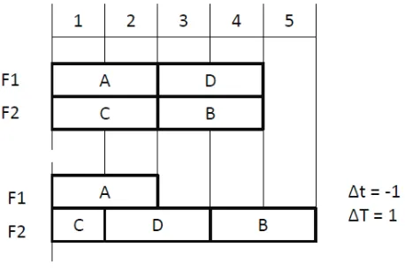
Consider a processor with two functional units F1 and F2. F1⊂F2, i.e., F2 can execute a superset of the instructions that can be executed in F1.
Figure 2.1: Anomaly where ∆t >0 results in ∆T >∆t
units F1 and F2, respectively. They finish execution in cycle 2 making operands ready for instructions B and D, respectively. In cycle 3, B is issued to F2 (since it can run only on F2) and D to F1. The sequence takes 5 cycles to execute. Now consider what happens when A takes 3 cycles to execute instead of 2. The entire sequence takes 7 cycles. This is an anomaly because an increase in the execution time of A by 1 cycle (∆t= 1) resulted in the whole sequence taking 2 cycles (∆T = 2) more.
Figure 2.2: Anomaly where ∆t <0 results in ∆T >0
Figure 2.2 shows another anomaly. Here, reduction in the execution time of C by 1 cycle results in the whole sequence taking 1 more cycle to execute.
2.2.3 Domino Effects
A domino effect is a phenomena where a small interference at the beginning of a sequence can result in an unbounded increase in run time. Lundqvist and Stenstrom [17] were the first to give an example of a domino effect. Berg [20] showed that a small change in cache state (and not necessarily the pipeline state) can result in domino effects. Domino effects have an interesting side effect — the overall runtime of a loop cannot be extrapolated using the run-time of the first few iterations of the loop. This is because a slight change in instruction scheduling can affect the execution of the the rest of the loop.
2.2.4 Timing Anomalies and WCET analysis
Hitherto, I have defined and given examples of timing anomalies. In this section, I will discuss the effects of timing anomalies on traditional WCET analysis methods.
Static timing analysis takes into account the architecture (pipeline) and the in-struction set. Given a program (usually in assembly), the technique computes the WCET by performing pipeline analysis at the instruction and the basic block level. Later, the WCETs of the basic blocks are combined to provide the WCET of the entire program. Also, whenever a variable latency instruction is encountered, its execution is emulated us-ing its maximum latency. This follows from the assumption that the local worst case always leads to a global worst case. Similarly, if a cache access cannot be classified as a hit or a miss, a cache miss is assumed. It has to be noted that, because of the nature of the analy-sis, these decisions are made at the instruction or basic block level. However, with timing anomalies, the assumption is no longer true. It is impossible to determine the exact latency of a variable latency instruction that results in the global worst case at the basic block level4
. Also, timing anomalies manifest at run-time and the impact may be enhanced by dynamic scheduling decisions. Such considerations are beyond the scope of static analysis. Hence, static analysis cannot provide safe bounds for architectures that exhibit timing anomalies. Dynamic timing analysis also has issues addressing timing anomalies. For variable-latency instructions whose execution time depends on the actual inputs, the analysis has to not only consider all inputs but also all combinations of inputs. Cache states also impact analysis. It has been shown that timing anomalies and and even domino effects can occur as a result of cache behavior [5, 20]. Current dynamic analysis techniques, typically, do not consider cache states while determining WCET. Hence, dynamic analysis falls short of
4
providing safe bounds on processors exhibiting anomalies.
2.3
WCET techniques to address anomalies
A lot of research has been done to provide safe estimates for out-of-order archi-tectures. One approach is the use of a Virtual-Simple Architecture (VISA) [21]. In this technique, any task that is run on the complex processor is divided into sub-tasks and dead-lines for the sub-tasks are verified at run-time using checkpoints. If a checkpoint is missed, the processor is likely to miss the deadline for the task, and hence, the out-of-order processor is switched to a simple-mode within VISA. The simple-mode provides predictable execution using an in-order pipeline. The WCET analysis for the task is performed on the simple VISA pipeline using traditional static timing analysis technique. Hence, the approach pro-vides predictable execution on out-of-order architectures effectively circumventing direct WCET analysis on them.
Jack Whitham and Neil Audsley take another approach to predictable execution on complex architectures [22]. In their technique, execution by an out-of-order processor is made predictable through trace-based execution. During trace based execution, the CPU is controlled by a Virtual Trace Controller (VTC). These and other architectural enhancements avoid timing anomalies by eliminating sources of timing noise in the pipeline making WCET analysis safe.
2.4
Summary
Chapter 3
Hybrid Timing Analysis through
CheckerMode
3.1
Introduction
The previous chapter discussed the drawbacks of static and dynamic analysis tech-niques. This chapter presents a new technique, categorized as hybrid timing analysis, that aims at addressing the drawbacks of static and dynamic analyses. Unlike static analysis, the presented technique can analyze out-of-order architectures. Unlike dynamic analysis, the technique can provide safe bounds. Also, the technique can analyze processors that exhibit timing anomalies, if resources are assigned statically.
The thesis is a continuation of prior related work [6, 23, 7]. The rest of the chapter is organized as follows. Section 3.2 provides an overview of the technique. Section 3.3 delineates my contributions from prior work. Section 3.4 states the assumptions. Section 3.5 discusses the desing and implementation. Section 3.6 discusses how timing anomalies are handled by the technique. Section 3.7 discusses the WCET estimates obtained using the technique.
3.2
Overview
is estimated by running the task on the actual processor. Like the static analysis technique, hybrid analysis constructs control-flow graphs and uses them to direct the actual execution on the processor ensuring that all paths are exercised before determining the WCET. This ensures that the WCET is safe.
In order to estimate the WCET of a task, it is run on a special mode of the proces-sor calledCheckerMode. Running a task inCheckerMode is different from running it under the normal deployment mode (the behavior of the processor is unaltered in the deployment mode). CheckerMode supports timing analysis and requires certain architectural enhance-ments (Section 3.5). In CheckerMode, all paths of the task are systematically executed and timed one after the other. Specifically, whenever a conditional branch is encountered, the processor executes (and times) both the taken and the not-taken paths. The alternate paths are executed in isolation from each other usingsnapshots. Snapshots capture proces-sor pipeline information. When alternate paths join, the pipeline snapshots at the join are merged to produce a snapshot that depicts the effective processor state at the join. The largest execution time up to that point and the merged snapshot are used for timing the rest of the task.
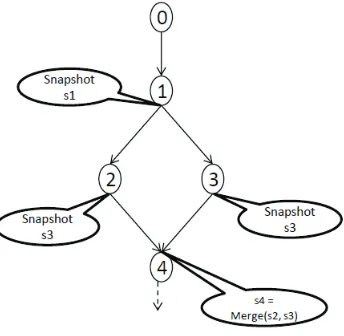
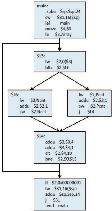
Figure 3.1: A Simple CFG.
execution continues through one of the paths, say 1→2 and another snapshot,S2, is taken at the end of it. To time the other path, snapshotS1 is restored and execution is restarted from the beginning of basic block 1. Restoring snapshot S1 ensures pathological timing behavior. Execution continues down the other path, 1 → 3 and another snapshot S3 is taken. Before proceeding through basic block 4, snapshotsS2 andS3 are merged to obtain snapshot S4. Now, snapshot S4 needs to be restored before continuing down basic block 4. The two paths are timed during execution, the longer of which is used for the WCET estimate.
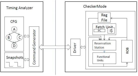
Figure 3.2: CheckerMode Block Diagram.
During the timing of the entire task, the CheckerMode is assisted by a timing analyzer (TA) and a CheckerMode driver. Figure 3.2 shows the block diagram.
The setup consists of two parts, a TA and a CheckerMode processor. The TA is shown on the left side of the block diagram. Given a task (program) in assembly1
, it breaks down the task into basic blocks2
and constructs control-flow graphs (CFGs). The TA uses the CFGs and generates commands, which in turn drive the execution in CheckerMode, as shown in Figure 3.1. The TA stores the snapshots in a snapshot buffer. It times the various paths and derives the WCET estimate. The CheckerMode architecture is shown on the
1
An executable can be disassembled and used to the same effect.
2
right side of Figure 3.2. It consists of a driver that uses the commands issued by the TA and drives the processor pipeline. The pipeline itself is enhanced so that the it can capture and restore snapshots. More details of CheckerMode operation are provided in Section 3.5.
3.3
Contributions of this thesis
Hybrid timing analysis using CheckerMode has been discussed in a number of publications [6, 23, 7, 8]. This section delineates the contributions of this thesis from existing work.
CheckerMode [6, 23, 7] devised the initial snapshot capture, restore and merge tech-niques and proved that the technique preservers timing anomalies. This thesis continued the work, completing the implementation of snapshot capture on the SimpleScalar simula-tor.Snapshot merge and restore techniques were implemented. A command language, for the interaction between the TA and CheckerMode processor, was developed. SimpleScalar was transformed from a program-driven processor to one that responds to the command language described in Section 3.5.2.
3.4
Assumptions
In this research, we are concerned with analyzing out-of-order pipelines. The behavior of caches is known to affect WCET estimates of a task [20]. However, behavior of caches or the complete memory hierarchy in general are not considered in this work. Similarly, the effect of branch prediction is also not not analyzed. Tasks are analyzed in isolation.
The WCET analysis is done during pre-deployment. Overall performance of the hardware during timing analysis is not considered critical. On the other hand, we have tried to keep the hardware enhancements to a minimum.
not modified. It has to be noted that we are only concerned about the timing behavior of the program (during analysis) and not about its logically-correct behavior (in terms of I/O relations). The program needs to be tested for its logical correctness independent of timing analysis.
3.5
Design and Implementation
This section discusses the design and implementation of the hybrid timing analysis technique. Section 3.5.1 discusses the architectural changes required to support Checker-Mode execution on an out-of-order processor. Section 3.5.2 discusses the timing analyzer that generates commands for obtaining WCET bounds.
3.5.1 Hardware Enhancements: CheckerMode
As stated earlier, during timing analysis, the program analyzed is run in a special mode of the processor called CheckerMode. Any inputs that the program takes are deemed unknown and conceptually denoted as a special top value, NaN (not-a-number), similar to the special value used in floating-point units. If one operand of an instruction is unknown, the result is unknown. For example, multiply is redefined as follows:
rresult{N aN if r
a=N aN or rb=N aN
ra∗rbotherwise (3.1)
The reason for using NaNs become apparent while analyzing variable latency in-structions (inin-structions whose execution time depends on their operands). Pathological timing behavior is enforced on variable latency instructions operating on NaNs so as to ensure safe WCET bounds.
During CheckerMode execution, the control flow is determined by the TA and not the program’s inputs. The behavior of certain control-transfer instructions (conditional branches) were modified appropriately.
At the core of hardware enhancements is the ability to capture, restore and merge snapshots. As stated before, a snapshot saves processor state along with some timing information. A snapshot
1. preserves structural and data dependencies across instructions belonging to adjacent basic blocks;
2. preserves timing anomalies and pathological timing behavior for static resource as-signments;
3. provides path isolation while running alternate paths; and
4. reduces the number of combinations of paths that need to be timed in order to deter-mine the WCET of a task.
Above, 1 and 2 are very much interrelated. Timing anomalies can be preserved by maintaining structural and data dependencies across instructions belonging to different basic blocks. More information about preserving timing anomalies is provided in Section 3.6.
Details of the snapshot capture, restore and merge have been published earlier [23, 7]. There is some overlap in the concepts presented, mainly for completeness of discussion. However, the discussion provided in this thesis is more relevant to the SimpleScalar pipeline.
Snapshot Capture
It was stated earlier that snapshots contain pipeline state and timing information. The state information includes the following:
• the PC at which the snapshot is taken;
• the state of the register file; and
Additionally, the state information may contain any other architecture specific information that is used to restart execution form the snapshot. For example, for SPARC architecture, this includes the state of the register window mechanism.
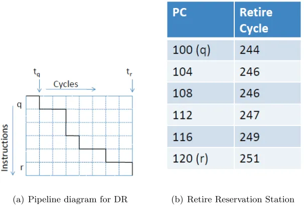
The timing information in the snapshot is captured using a minimally intrusive procedure called the Drain-Retire (DR) technique. Instead of capturing the state of each instruction in each stage of the pipeline (which would be very intrusive), the DR-technique captures only the retire times of each instruction. An example makes the idea clear.
Figure 3.3: Analysis Model for the DR technique
(a) Pipeline diagram for DR (b) Retire Reservation Station
Figure 3.4: Drain Retire Technique for Snapshot Capture
of the data captured by the DR technique. Figure 3.4(b) shows the actual data structure, referred to as the retire reservation station.
Structural and Data Dependencies
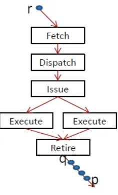
The snapshot capture and restore mechanism has to maintain structural and data
dependencies across instructions belonging to different basic blocks so as to keep the WCET
estimates safe. An example makes the point clear. Consider Figure 3.6. It shows
instruc-tions p and q belonging two different basic blocks A and C, respectively. Let q be data dependent on p. During normal execution,q stalls in the pipeline until p completes execu-tion. Letta,tb and tc be the WCET estimates of the basic block A, B and C, respectively.
Combined WCET of basic blocks A and C, without considering the stall time of instruction q then amounts to:
(T1) =ta+tc (3.2)
Combined WCET of basic blocks A and C, taking q’s stall time into account is:
Figure 3.5: Dependencies.
Combined WCET of basic block B and C is:
(T2) =tb+tc (3.4)
Overall, WCET bound depends onq’s stall time if:
T1< T2< T1′ (3.5)
Equations (3.2), (3.3), (3.4), (3.5) build up a specific situation when the WCET estimate would be incorrect if the data dependency betweenp and q is not captured. Also, it has to be noted that the same example would hold if there were to be a structural dependency between p and q instead of a data dependency. Hence the snapshot capture technique must account for structural and data dependencies.
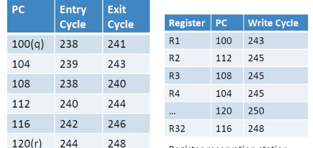
Capturing Structural Dependencies
In order to capture structural dependencies, a data structure calledIssue Reserva-tion StaReserva-tion, shown in Figure 3.6(a)3
is used. It captures the utilization of each functional unit per instruction. One drawback of the design is that the program counter (PC) is used
3
(a) Issue Reservation Station (b) Register Reservation Station
Figure 3.6: Capturing Structural and Data dependencies
to identify instructions. As a side effect, it is not possible to distinguish between different dynamic instances of a single instruction in a loop. The TA will have to run only one iteration at a time. This design was chosen in order to keep hardware extensions to a minimum.
Capturing Data Dependencies
Data dependencies are tracked using a data structure called Register Reservation Stationshown in Figure 3.6(b)3
. This data structure stores, for each register, the instruction that updates the register (PC) and the register write cycle. In architectures that use register renaming [24], this data structure maintains one entry for each logical register instead of for each physical register4
.
To summarize, the snapshot capture mechanism records:
• the PC at which the snapshot was captured;
• the snapshot capture cycle;
• register file state at the end of Drain-Retire;
4
• retire times of all instructions in the pipeline (using the DR technique);
• functional unit usage times of the same set of instructions (captures structural depen-dencies); and
• register usage information that can determine any data dependencies with future instructions that enter the pipeline.
Snapshot Restore
It was stated earlier that a snapshot
• preserves structural and data dependencies across instructions belonging to adjacent basic blocks; and
• preserves pathological timing behavior.
The snapshot restore mechanism uses the information recorded in the snapshot to enforce the above conditions. Consider Figure 3.3. It has to be noted that the snapshot capture mechanism has recorded the retire times, functional unit usage times and register usage times of all instructions, q through r. The idea is to delay the execution of instructions following r such that any potential structural and data hazards are maintained. This is enforced by restarting execution from the previous snapshot5
and carefully replaying the execution of instructions from q through r using the snapshot information. Specifically, instructions from q through r are not allowed to exit the reservation stations earlier than as specified by the snapshot. The instructions cannot use the register values earlier than, as recorded in the snapshot. Instruction retire time-stamps are also enforced6
. The snapshot restore mechanism requires hardware modifications to manage the instruction flow in the pipeline as specified by a snapshot.
Some readers may question as to how the restore mechanism is much different com-pared to simply restarting execution at an earlier point and continuing normal instruction execution down a specific path. There are two key differences.
5
Execution may be restarted from instruction q. However, since the timing analysis is being performed on an out-of-order architecture, restarting from q may result in loose bounds. Execution is restarted from the previous snapshot, enabling the pipeline to fill up while the snapshot instruction is reached.
6
• Snapshot/restore preserves pathological timing behavior. Between the initial run and the replay, the pathological case is automatically considered for the WCET estimate.
• More importantly, once the snapshot information is captured, it may be altered (say, by a snapshot merge technique explained below) and the restore mechanism will ensure reliable replay as defined by the new snapshot. The snapshot merge technique enables snapshot restore atjoin points as shown in Figure 3.1.
Snapshot Merge
Figure 3.7: Merge of two paths
Consider Figure 3.7. Paths blocks A and B end with SnapshotsSAandSB
respec-tively. Before continuing execution of instructions from path C, SA and SB are merged to
produce snapshot SM. The merge technique will combine the pipeline timing information
from the two snapshots. The restore of snapshotSM ensures that, while executing
instruc-tions from path C, the structural and data dependencies from either paths (A and B) are maintained. The snapshot merge technique has been proved to preserve timing anomalies [23, 7].
The thesis describes the merge of retire reservation stations, issue reservation sta-tions and register reservation stasta-tions for completeness. More information about snapshot merge can be obtained from [23, 7].
Drain-Retire Merge
The merge of two retire reservation stations follows a simple algorithm described below.
Figure 3.8: Drain-Retire Merge
Figure 3.9: Merging Issue Reservation Stations
2. Find a set B of instructions in the other reservation station that retire earliest (among all instructions in the second reservation station). Each set will contain a minimum of one instruction.
3. The union of the sets A and B now retire at the maximum of the two retire times in the merged reservation station.
The above set of steps are applied until no instruction is left in either reservation station. An example is provided in Figure 3.8.
The above algorithm ensures that when the merged snapshot is restored (figure 3.7), instructions from path C are automatically delayed until the longer of the paths complete.
Merging Issue Reservation Stations
Merging of issue reservation stations is best demonstrated by an example (Figure 3.9). The maximum entry cycle and maximum exit cycle for each reservation station entry is used in the merged result.
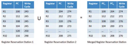
Merging Register Reservation Stations
Figure 3.10 shows the merge of two register reservation stations. The later of the update times of each register is used in the merge result.
3.5.2 Timing Analyzer
Interaction Between the timing analyzer and CheckerMode Driver
Using the CFG, the TA sends commands to the CheckerMode driver. The driver executes the commands using the CheckerMode hardware and sends back the results. The results are used for the WCET estimate. This section discusses the command language that is used for communication between the TA and the CheckerMode driver.
Commands can be classified into two groups:
(I) Setup Commands: These commands populate the pipeline. No instructions are executed in the pipeline as a result of these commands.
(II) Execution Commands: These commands trigger execution of instructions from the current state of the pipeline. The state itself is only influenced by setup commands. Results from the execution are returned to the TA.
Setup Commands
The setup commands are:
1. put snapshot<Snapshot ID>: This command restores a snapshot. The snapshot
to restore is identified by a unique snapshot ID. If the snapshot is not cached by the CheckerMode driver, the CheckerMode driver obtains the snapshot from the TA which has a larger buffer that stores all previous snapshots.
2. put timing <Snapshot ID>: This command replays a snapshot identified by
<Snapshot ID>. If the snapshot is not cached by the CheckerMode driver, it is obtained from the TA.
3. put PC <Branch PC><Next PC><T/NT>: This command overrides the
outcome of control flow instructions and thereby forces branches to evaluate such that control flow is directed along the desired path. It has three arguments: the branch PC, the PC of the target instruction and the branch outcome — taken/not taken.
Execution Commands
These commands result in execution of instructions through the pipeline.
1. get snapshot <Snapshot PC>: The command captures snapshots. It initiates
execution from the current “state” of the pipeline. The “state” itself is affected by the commands above. When <Snapshot PC>is fetched from the instruction stream a snapshot is captured and returned to the TA. Note that a PC specification does not uniquely identify a single point during program execution. PCs repeat iteratively within loops or when functions are called at different call sites (or within loops). However, snapshots have to be uniquely identified with points during program execu-tion. This is realized by ensuring that all “put PC” commands are completed before a unique point in execution is reached and a snapshot is captured. For example, in order to take a snapshot at the beginning of the third iteration of a loop the “put PC” command is issued twice before the “get snapshot” command. The two “put PC” directives steer execution into the third iteration of the loop before a snapshot is captured.
2. get timing<PC1><PC2>: This command captures execution times for program
paths. Execution of instructions is initiated from the current “state”. Subsequently, the time taken to execute all instructions between the specified PCs (and hence for that particular path) is returned to the TA.
3.6
Timing Anomalies and Hybrid Timing Analysis
However, the technique has a drawback. NaNs were introduced to handle the timing behavior of variable latency instructions. Variable latency instructions with NaN operands are forced to exhibit pathological timing behavior during analysis. This is done in order to ensure safeness of the WCET bound. However, such a mechanism is a classic example of the assumption that a local worst case leads to a global worst case, and may produce unsafe bound in the presence of timing anomalies.
One way to solve the issue is to ensure static allocation of resources: each in-struction in the program has to be allocated statically to the same functional unit across multiple executions of the program. The solution follows from the Resource Allocation Criterion (RAC) [18].
3.7
Results
The hardware enhancements from Section 3.5.1 were made to a processor simulator called SimpleScalar [25]. SimpleScalar supports both in-order and out-of-order execution of instructions. The processor features the PISA (Portable Instruction Set Architecture) instruction set, which is similar to the MIPS ISA. The authors also provide a GCC cross compiler for PISA and associated tools [26]. Enhancements were made to SimpleScalar to capture snapshots, restore snapshots and merge them. SimpleScalar was also modified from being program driven to being command driven.
The experimental setup is similar to the block diagram shown in Figure 3.2. The TA generates the commands (Sections 3.5.2 and 3.5.2) and the CheckerMode infrastructure executes the commands thus generating the WCET results. In order to restore a snapshot (Section 3.5.1) at a particular point in the program, execution is restarted from an earlier point and the snapshot at the point of restore is replayed. For the tightest bounds possible using this technique, the point of restart should be far enough back to let the pipeline be filled completely with instructions by the time the restore point is reached. However, in this section, we restart execution from the previous snapshot for simplicity. Also, there is no static allocation of instructions to functional units as noted in Section 3.6. Hence, the current implementation does not preserve all anomalies.
simplest benchmark to exercise the snapshot merge. toy consists of an if-then-else block with a simple loop in the else block. cnt counts the number of positive and negative integers in an array of size 10. factorial calculates 5! andfibonacci determines the Fibonacci number of 30. cnt,factorial and fibonacci are from the C-Lab benchmark suite [27].
SimpleScalar has separate instruction and data caches at L1 stage and a com-bined L2 cache. Both were disabled as cache behavior is beyond the scope of this work. SimpleScalar uses dynamic branch prediction and speculative execution, which are again non-deterministic. Since there is no simple way to turn off branch prediction, perfect predic-tion was used. Perfect predicpredic-tion works by obtaining the branch targets from a funcpredic-tional simulator (within SimpleScalar) that runs ahead of the timing simulator.
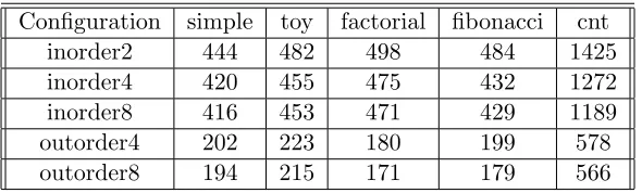
Table 3.1 shows the WCET bounds for each benchmark. The benchmarks were run in both in-order and out-of-order configurations of the simulator. Each row in the table specifies a particular configuration. For example, row 1 (inorder2) lists the results for an in-order configuration with a pipeline width of 2, i.e., the fetch rate, the dispatch rate, the issue width and the retire width were all set to 2. Similarly, row 4 shows results for an out-of-order configuration with a pipeline width of 4. All configurations use an ROB of size 64 and an issue queue of size 16.
Table 3.1: WCET bounds on CheckerMode Configuration simple toy factorial fibonacci cnt
inorder2 444 482 498 484 1425
inorder4 420 455 475 432 1272
inorder8 416 453 471 429 1189
outorder4 202 223 180 199 578
outorder8 194 215 171 179 566
It may be noted that the WCET bound for cnt is considerably larger than that of other benchmarks. The CFG ofcnt features an if-then-else path within a loop requiring a merge at the end of each iteration. Such a CFG can be considered as a worst-case input for our analysis technique. Consequently, our technique produces relatively loose WCET bounds for such input program.
3.8
Summary
Chapter 4
CheckerCore: Enhancing FPGA
Softcore for WCET Analysis
4.1
Introduction
The previous chapter discussed hybrid timing analysis through CheckerMode. One of the criticisms of CheckerMode has been that the enhancements are made to a processor simulator. Mohan’s dissertation [7] discusses the feasibility of hardware enhancements to modern processors. To make a more convincing arguments about the plausibility of the CheckerMode approach, researchers at Penn State University (PSU) and North Carolina State University (NCSU) worked on an FPGA Soft Core enhancement that can perform WCET analysis. Work on the FPGA soft core was done at PSU and the software compo-nents were developed at NCSU. This chapter gives an overview of the methodology without going into the implementation details of the hardware. For a more detailed discussion, the readers are referred to [8]. The chapter is organized as follows. Section 4.2 gives an overview of the CheckerCore system. Section 4.3.1 discuss the WCET analysis results.
4.2
Overview of CheckerCore
Figure 4.1: CheckerCore framework
TA is responsible for deriving the WCET of a program. It uses the program disassembly to construct a control flow graph (CFG). The CFG is then used to drive the back-end to measure the timing of all paths of the program. These timing values are combined to find the longest path(s) in the program and then derive the overall WCET. The back-end is a physical processor with support for a CheckerMode whose purpose is to support check-pointing and restarting executions while preserving timing. In this paper, such a mode was implemented within CheckerCore, an extension to an FPGA soft-core.
The TA used here is essentially the same that was used with the CheckerMode sim-ulator, except for minor modifications. The CheckerMode, built on top of the simplescalar simulator runs PISA instruction set. The FPGA softcore ran SPARC instructions. Hence the TA was enhanced to work with SPARC programs. The standardized communication API 3.5.2 was useful here.
drives the hardware during WCET analysis, and a snapshot buffer that caches snapshots.
4.3
Experiments and Results
4.3.1 Experimental Setup
The baseline architecture is configured to support the full SPARC V8 specification, except for co-processor and floating-point instructions. Both the I-cache and D-cache are also turned off and, as explained previously, we stall all memory instructions for a pre-programmed number of cycles. Cache and memory analysis is orthogonal to our framework and can be added as part of future work.
The enhancements applied to the baseline architecture and implemented on a Xil-inx ML505 FPGA evaluation board, which hosts a XilXil-inx Virtex 5 FPGA chip (XC5VLX110T). We connect the board to a computer using the 10/100 Mbps Ethernet physical interace and use the Ethernet debug interface shown in Figure 3.2 for communication between the front-end and the back-front-end.
WCET Estimation Results
We derive the WCET estimation of 6 benchmarks. (Table 4.1): simple andtoyare synthetic benchmarks that we constructed;cnt,bs,factorial, andfibonacci are from C-Lab benchmark suite [27]. Benchmark simple has only an if-then-else block. It is the simplest benchmark that exercises our merge algorithm. Benchmark toy has a simple if-then-else block and a loop of 10 iterations within the else block. The CFG of toy is a bit more complex than simple but requires fewer snapshot merges than cnt. Benchmark cnt finds the sum of positive and negative numbers in an array of size 10. Benchmarkbs is a binary-search in an array of size 15 elements. Benchmarkfactorial finds 5! using an iterative loop. Benchmark fibonacci finds the fibonacci number of 30 using an iterative loop. To execute each benchmark, we first fast-forward to the start of the “main” function, and then start the process of capturing the WCET until the end of that function. Fast-forwarding is enabled by CheckerCore. Anew command to initiate fast-forwarding is added to the driver besides those mentioned in the command language API (Section 3.5.2).
set of results to study the impact of memory latency. Rows 2-5 of the table show four sets of results corresponding to the memory stall cycles of 0, 8, 16, and 32, respectively. This is carried out for all six benchmarks. We notice that for all the benchmarks the WCET increases, as expected, with the increased memory latency.
Table 4.1: WCET bounds on CheckerCore Stall
simple cnt bs factorial fibonacci toy Cycle
0 173 6610 2029 467 623 2139
8 188 7258 2134 563 886 2434
16 224 8500 2682 722 936 3022
32 309 11484 3874 1066 1336 4189
Chapter 5
Conclusion
Static timing analysis provides safe and tight bounds for simple in-order pipelines but fails for more complex processors with out-of-order and speculative execution. Dynamic timing analysis can analyze such complex processors but fails to provide tight bounds. Neither of the analysis techniques is applicable to processors that exhibit timing anomalies. This thesis discusses a hybrid timing analysis technique that aims to provide safe and tight bounds for complex out-of-order processors that exhibit timing anomalies.
Hybrid timing analysis technique involves both hardware and software enhance-ments. Hardware enhancements included the ability to:
• capture, restore and merge snapshots; and
• steer execution by a combination of control-transfer instructions and external com-mands.
The software, also called the timing analyzer, divides the program into control-flow graphs and uses them to systematically execute and time alternative paths in the program to calculate the WCET bounds.
In order to make a more convincing arguments about the plausibility of the Check-erMode approach, the thesis demonstrated timing analysis using CheckerCore, a mode en-hanced FPGA soft-core.
timing anomalies, the handling of NaNs in the pipeline may result in unsafe bounds in the presence of anomalies. One solution to this problem has been discussed.
Bibliography
[1] Wikipedia. Anti-lock Braking System (ABS), 2008.
[2] J. Liu. Real-Time Systems. Prentice Hall, 2000.
[3] R. M. Tomasulo. An efficient algorithm for exploiting multiple arithmetic units. pages 13–21, 1995.
[4] James E. Smith. A study of branch prediction strategies. In ISCA ’98: 25 years of the international symposia on Computer architecture (selected papers), pages 202–215,
New York, NY, USA, 1998. ACM.
[5] Thomas Lundqvist and Per Stenstrom. Timing anomalies in dynamically scheduled microprocessors. Real-Time Systems Symposium, IEEE International, 0:12, 1999.
[6] Sibin Mohan and Frank Mueller. Hybrid timing analysis of modern processor pipelines via hardware/software interactions. In IEEE Real-Time Embedded Technology and Applications Symposium, pages 285–294, 2008.
[7] Sibin Mohan and Frank Mueller. Merging state and preserving timing anomalies in pipelines of high-end processors. In IEEE Real-Time Systems Symposium, December 2008.
[8] Jin Ouyang, Raghuveer Raghavendra, Sibin Mohan, Tao Zhang, Yuan Xie, and Frank Mueller. Checkercore: enhancing an FPGA soft core to capture worst-case execution times. InCASES ’09: Proceedings of the 2009 international conference on Compilers, architecture, and synthesis for embedded systems, pages 175–184, New York, NY, USA,
[9] J. Engblom.Processor Pipelines and Static Worst-Case Execution Time Analysis. PhD thesis, Dept. of Information Technology, Uppsala University, 2002.
[10] S. Mohan, F. Mueller W. Hawkins, M. Root, D. Whalley, and C. Healy. Paramet-ric timing analysis and its application to dynamic voltage scaling. page (accepted), September 2007.
[11] F. Mueller. Timing analysis for instruction caches. 18(2/3):209–239, May 2000.
[12] Iain Bate and Ralf Reutemann. Worst-case execution time analysis for dynamic branch predictors. InECRTS ’04: Proceedings of the 16th Euromicro Conference on Real-Time Systems, pages 215–222, Washington, DC, USA, 2004. IEEE Computer Society.
[13] V. Braberman, M. Felder, and M. Marre. Testing timing behavior of real-time software. 1997.
[14] Joachim Wegener and Matthias Grochtmann. Verifying timing constraints of real-time systems by means of evolutionary testing. Real-Time Syst., 15(3):275–298, 1998.
[15] Joachim Wegener and Frank Mueller. A comparison of static analysis and evolutionary testing for the verification of timing constraints. Real-Time Syst., 21(3):241–268, 2001.
[16] Reinhard Wilhelm, Jakob Engblom, Andreas Ermedahl, Niklas Holsti, Stephan Thesing, David Whalley, Guillem Bernat, Christian Ferdinand, Reinhold Heckmann, Tulika Mitra, Frank Mueller, Isabelle Puaut, Peter Puschner, Jan Staschulat, and Per Stenstr¨om. The worst-case execution-time problem—overview of methods and survey of tools. ACM Trans. Embed. Comput. Syst., 7(3):1–53, 2008.
[17] Thomas Lundqvist. A WCET analysis method for pipelined microprocessors with cache memories. 2002.
[18] I. Wenzel, R. Kirner, P. Puschner, and B. Rieder. Principles of timing anomalies in superscalar processors. In Quality Software, 2005. (QSIC 2005). Fifth International Conference on, pages 295–303, September 2005.
Frank Mueller, editor, 6th Intl. Workshop on Worst-Case Execution Time (WCET) Analysis, Dagstuhl, Germany, 2006. Internationales Begegnungs- und
Forschungszen-trum f”ur Informatik (IBFI), Schloss Dagstuhl, Germany.
[20] Christoph Berg. PLRU cache domino effects. In Frank Mueller, editor, 6th Intl. Workshop on Worst-Case Execution Time (WCET) Analysis, Dresden, number 06902
in Dagstuhl Seminar Proceedings. Internationales Begegnungs- und Forschungszentrum fuer Informatik (IBFI), July 2006.
[21] Aravindh Anantaraman, Kiran Seth, Kaustubh Patil, Eric Rotenberg, and Frank Mueller. Virtual simple architecture (VISA): exceeding the complexity limit in safe real-time systems. SIGARCH Comput. Archit. News, 31(2):350–361, 2003.
[22] Jack Whitham and Neil Audsley. Predictable Out-of-order Execution Using Virtual Traces. InProc. RTSS, pages 445–455, 2008.
[23] S. Mohan. Exploiting Hardware/Software Interactions for Analyzing Embedded Sys-tems. PhD thesis, Dept. of CS, North Carolina State University, August 2008.
[24] Mayan Moudgill, Keshav Pingali, and Stamatis Vassiliadis. Register renaming and dynamic speculation: an alternative approach. InMICRO 26: Proceedings of the 26th annual international symposium on Microarchitecture, pages 202–213, Los Alamitos,
CA, USA, 1993. IEEE Computer Society Press.
[25] D. Burger, T. Austin, and S. Bennett. Evaluating future microprocessors: The sim-plescalar toolset. Technical Report CS-TR-96-1308, University of Wisconsin - Madison, CS Dept., July 1996.
[26] SimpleScalar LLC. Simplescalar tools, 2004.