Analysis and experimental evaluation of rate adaptation with transmit buffer information

(1)

R E S E A R C H

Open Access

Analysis and experimental evaluation of rate

adaptation with transmit buffer information

Yongjiu Du

*

, Dinesh Rajan and Joseph Camp

Abstract

In hardware, packet loss may happen due to overflow at a finite-depth transmit buffer in addition to the packet corruption in the channel. To reduce such losses and further improve spectral efficiency via rate selection, we exploit either statistical or instantaneous knowledge of transmit buffer occupancy and source packet distribution in

IEEE 802.11-based systems, which have highly variable frame durations. We consider a traditional method of rate adaptation based on channel quality information and evaluate the throughput gain in hardware when the buffer occupancy and source packet distribution information are known. Our optimization objective is to maximize the throughput with constant transmit power since most wireless standards (e.g., 802.11, Bluetooth, ZigBee) operate in this manner. We study both cases with and without probe packets during the transmission. By evaluating the effect of diverse buffer sizes with different packet arrival distributions, both our theoretical analysis and our experimental results show that the throughput can be improved as much as 35% when the source packet distribution and buffer status information are exploited.

Keywords: Rate adaptation; Transmit buffer information; Markov chain; SNR; FPGA; Implementation

1 Introduction

Rate adaptation is widely used to increase spectrum efficiency in time-varying wireless channels. Packet loss/success-based rate adaptation protocols have been well studied and widely implemented in the past decade [1-5]. This kind of protocol uses packet loss/success statistics to select the perceived best rate to transmit data packets. However, packet-level information is coarse-grained and usually takes tens of transmis-sions to get a reasonable estimate of the channel quality. As a result, the performance of loss-based rate adapta-tion protocols is known to degrade as the Doppler shift increases. To enable rate adaptation with high mobility, a variety of SNR-based rate adaptation protocols have been developed that can adapt to fast-fading channels [6-9]. However, the SNR is not always an accurate indicator of packet error rate (PER) for orthogonal frequency division multiplexing (OFDM) systems in frequency-selective channels. To address this problem, soft information from SISO (soft-in soft-out) decoders has been used to deter-mine the best rate, which has a much better performance

*Correspondence: [email protected]

Department of E.E., Southern Methodist University, Dallas, Texas, 75206, USA

in multi-path channels [8]. Additional improvements have come from a novel effective signal-to-noise ratio (SNR) metric for rate adaptation, achieving better perfor-mance than protocols that are solely based on SNR [9]. These SNR-based schemes have yet to be widely used in commercial systems.

Traditional rate adaptation protocols usually assume a fully backlogged transmit buffer. However, in real hard-ware, the buffer depth is always finite and the buffer occu-pancy is time-varying. The packet loss in a system without retransmissions results from either packet overflow at the transmit buffer, receive buffer, or packet corruption in the channel. Note that the wired network connected to the receiver usually has a much higher capacity than the wire-less channel, which could prevent packet overflow at the receive buffer. Consequently, using both transmit buffer information and channel information for rate adaptation may achieve superior performance [10-14]. These works use either statistical or instantaneous information of the buffer occupancy and channel quality to adaptively change the transmission rate, which allows significant perfor-mance gain. However, all of these works aforementioned leverage simulation to illustrate the importance of buffer status information without implementation in hardware,

(2)

which may lead to a less accurate evaluation of the sys-tem’s complexity and channel activity. Moreover, each work assumes a constant frame duration, within which various packet numbers and/or sizes are sent for differ-ent rates to equalize the frame duration. Since the packet arrival probability and channel state transition probability during one frame highly depend on the frame duration, in these constant-frame-duration systems, both the packet arrival probability and the channel state transition proba-bility are much simpler than variable-frame-duration sys-tem. For HSPA (high-speed packet access) and DO (data optimized) systems in 3G networks, transmit buffer infor-mation and channel quality inforinfor-mation of the users are jointly used for user scheduling by the base station [15,16]. However, to the best of our effort, no publication was found considering buffer status information for rate adaptation in HSPA and DO systems. We acknowledge that proprietary buffer-assisted rate adaptation for HSPA could exist and be in operation in commercial devices. However, we are unable to implement and/or directly compare rate decisions of such schemes to our own.

In reality, many protocols use variable frame durations (e.g., IEEE 802.11, HIPERLAN/2, IEEE 802.15.3, ZigBee, and IEEE 802.16), which have been widely used in com-mercial applications. In these systems, only one packet is transmitted in each frame slot with a given packet size according to the application. As a result, the frame dura-tion in these protocols varies for different packet sizes and transmission rates. In this system model, the chan-nel state transition probability varies with different frame slot durations, and the frame slot duration depends on the buffer status. The packet arrival probability is also a vari-able for different frame slots. The varivari-able channel state transition probability and variable packet arrival proba-bility are essentially different from the existing constant-frame-duration systems. Therefore, we are not able to apply the optimization model of constant-frame-duration systems to variable-frame-duration systems. We will dis-cuss such a variable-frame-duration mechanism based on the IEEE 802.11 PHY standard in this paper, and the method and result described can be directly applied to other variable-frame-duration systems. Moreover, for many devices and low-cost transceivers, packet-level power adaptation is not available. Thus, we only discuss rate adaptation with constant transmit power in this work. In this paper, we optimize rate adaptation strategies with either statistical or instantaneous buffer information. For statistical buffer information, we use knowledge of offered load distribution, buffer size, and fading channel model, and leverage a steady-state analysis of a joint buffer and channel quality Markov chain to obtain the opti-mal set of rate adaptation thresholds. For instantaneous buffer information, we use the instantaneous occupancy information and offered load information and derive the

packet loss rate (including both packet overflow at the transmit buffer and packet corruption in the channel) for each rate to obtain the optimal rate adaptation thresh-old set for each buffer status. Then, before selecting the transmit rate, the transmitter first selects the threshold set according to the instantaneous buffer status and decides the optimal rate based on the instantaneous channel gain and selected threshold set.

The main contributions of our work are as follows:

1. We formulate and analyze a cross-layer rate adaptation system with variable frame durations, which is the prevalent scenario in commercial wireless networks.

2. We provide solutions for rate adaptation with the knowledge of either statistical buffer information or instantaneous buffer information. Furthermore, we also analyze systems either with or without packets which probe the channel quality, in combination with either statistical or instantaneous buffer status. We achieve as much as 7% throughput improvement in cases with probe packets, and a much larger improvement of 35% in cases without probe packets. 3. We use Matlab to obtain one set of optimal

thresholds based on our proposed model and use real hardware experiments to achieve another set of optimal thresholds empirically. We show that both sets of thresholds converge to nearly identical thresholds for rate adaptation in the same scenario. 4. We experimentally evaluate the throughput

performance and empirically verify the theoretical analysis on a diverse set of wireless channels. With buffer status information, we show the throughput improvement as much as 35% compared to systems without buffer status information.

The paper is organized as follows. Section 2 presents a system model based on the IEEE 802.11 PHY standard and theoretically analyzes the methodology to choose the rate adaptation thresholds to optimize the throughput. The methodology for both statistical and instantaneous buffer information is provided. The experimental evaluation sys-tem settings are introduced in Section 3. Compared to purely link-layer rate adaptation systems, we experimen-tally show that far better performance can be achieved by considering either statistical or instantaneous buffer infor-mation in Sections 4 and 5, respectively. Related work is presented in Section 6. Finally, in Section 7, some con-cluding remarks and suggestions for future research are presented.

2 System model

(3)

Figure 1Rate adaptation system with offered load distribution and buffer status provided.

as shown in Figure 1. Packets arrive from the higher lay-ers into the transmit buffer according to a certain random process (e.g., a Poisson or Bernoulli distribution). The transmitter selects a packet from the buffer and sends it over the channel with one of the transmission rates in each frame slot. The receiver demodulates and decodes the received signal and also estimates and sends the channel information back to the transmitter through the feedback channel.

In this paper, we use a constant transmission power, although there are several works that consider power adaptation [12,17,18]. Our results are applicable in the low-cost transmitters that usually use the default power settings and do not change the transmit power at a packet level.

2.1 Dynamic transmit rate

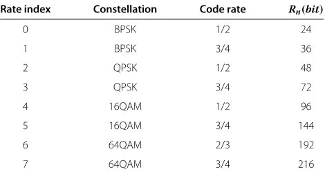
We use a frame structure as described in the IEEE 802.11 standard. One frame is composed of a short preamble, a long preamble, a header symbol, and several data sym-bols [19], as shown in Figure 2. Both the short preamble and the long preamble have a duration of two OFDM sym-bols. The header has a duration of one symbol. We assume the packet isLbytes. In the data symbols, there are 16-b service data and six convolutional code tail 16-bits. LetRn denote the number of data bits that can be transmitted in one OFDM symbol at raten, as shown in Table 1 [19]. The transmitter sends one packet every frame slot. The packet length could be from 1 to 2,047 B. The number of symbols in a frame is

Ns(n)= 5+

(8L+16+6) Rn

(1)

Let Ts denote the duration of one OFDM symbol. In this paper, we assume a constant payload size. Moreover,

if there are no packets in the buffer, the transmitter may still send probe frames that only include the preamble and header symbol to enable the receiver to continue to mea-sure the channel quality. The frame slot duration, Tf, is

Tf(m,n)=

5Ts+Td if m = 0

TsNs(n)+Td otherwise (2)

where Td is a fixed-time delay including demodulation, decoding, and feedback. The number of packets in the buffer equalsm.

The variation of PER with SNR,γ, for ratenis denoted by PERn(γ ). Since it is challenging to get a closed form expression of PERn in a coded system, we use the fol-lowing approximation from [14] to denote the PER as

PERn(γ )=min(1,anexp(−γ /gn)) (3)

wherean andgn are the parameters to describe PER for raten, andγ is the SNR value. The parameters for packet lengthL=1, 024 B are shown in Table 2.

2.2 Diverse offered load

In general, we assume that the packets arrive randomly at the buffer. Although long-range dependence in network traffic is well accepted in literature, recent studies show that current network traffic can be well represented by the Poisson model for sub-second time scales [20]. In this paper, we model the arrivals as a Poisson process with an average packet arrival rate ofλpackets per second. In one time intervalt, the probability ofkpackets arriving,

pK(K =k|t), is given by [21]

pK(K=k|t)=

(λt)k

k! exp(−λt) k=0, 1, 2. . . (4)

(4)

Table 1 Transmission rate parameters for IEEE 802.11 a/g systems

Rate index Constellation Code rate Rn(bit)

0 BPSK 1/2 24

Hence, during a packet transmission at raten, if there arempackets in the buffer, the probability ofk packets arriving,pK(K=k|m,n), is given by

pK(K =k|m,n)=pK(K=k|Tf(m,n))

= (λTf(m,n))k

k! exp(−λTf(m,n)) (5)

2.3 Dynamic channel quality

For the wireless channel, a Rayleigh fading model is a good approximation and agrees well with empirical obser-vations for mobile wireless links [22]. Let γ denote the received SNR. The distribution of γ can be expressed as [22]

whereγ¯is the expected value of SNR.

We divide the whole SNR region into N

non-overlapping regions. The number of feasible rates in which packets can be transmitted is alsoN. We define the thresh-olds asγ0 = 0 < γ1· · ·< γN = ∞. If the instantaneous SNR falls into the region betweenγnandγn+1, we say the channel is in statenand we use ratento transmit.

Assume pγn is the probability that the channel qual-ity falls into the region [γ_n,γ_n₊₁). We can calculatepγn

Table 2 PER approximation parameters for each rate in our system model

Rate 0 1 2 3 4 5 6 7

an 1.2 4 6 8 20 20 18 6

gn 1.8 1.2 1.3 2 2.8 7 20 50

For simplicity, we assume the channel is block-fading. LetCidenote the channel state in theith frame slot with a duration T. The channel keeps the current state or changes to the adjacent states according to the following crossover probability (as in [23,24]), which is suitable for slow-fading wireless channels.

Here, Nn is the level-cross-rate of the fading channel, denoted as [24] of the relative velocity between the transmitter and the receiver and the carrier wavelength.

(5)

2.4 Rate adaptation with statistical buffer information In this section, we investigate the offered load distribution, buffer size, and fading channel model. To do so, we lever-age a steady-state analysis of a joint buffer and channel quality Markov chain to get the optimal rate adaptation thresholds and apply this threshold set for rate adaptation. We model the buffer state transition as a queue service process. If we assume that the buffer is able to accom-modateMpackets, the buffer stateBi ∈ {0, 1, ...,M}. We assume(Bi,Ci)is the joint buffer and channel state. We then define a transition matrix P, as in (12), where the elementp(m,n)→(s,t) denotesp(Bi+1 = s,Ci+1 = t|Bi =

m,Ci = n), the transition probability from state(Bi =

m,Ci=n)to state(Bi+1=s,Ci+1=t).

Let πi,j denote the probability of buffer state i and channel statejand define the row vectorπas

π =[π0,0,. . .,π0,N−1,. . .,πM,N−1] (13)

For the steady state of this system, we have

π =πP (14)

and

0≤i≤M,0≤j≤N−1

πi,j=1 (15)

If the buffer is empty, the transmitter will send probe packets. Clearly, the transmitter will send a packet at the rate corresponding to the current channel state. Hence, the probability distribution of the next channel state depends on both the current channel state and the cur-rent buffer status. This dependence is essentially differ-ent from the constant-frame-duration model in previous works, in which the channel state transition probabil-ity only depends on the current channel state. Also, the buffer state transition depends both on the offered load distribution and the current channel state. Thus, we have

p(m,n)→(s,t)=p(Bi+1=s|Ci+1=t,Bi=m,Ci=n)

×p(Ci+1=t|Bi=m,Ci=n)

=p(Bi+1=s|Bi=m,Ci=n)

×p(Ci+1=t|Bi=m,Ci=n)

(16)

Now, we first discuss the buffer state transition proba-bilityp(Bi+1 = s|Bi = m,Ci = n). If the buffer is empty, the next state can be any state from 0 toM, and the buffer state transition only depends on the packet arrival pro-cess, as described by (5). If the incoming packets exceed M, all subsequent packets will be dropped due to over-flow. However, if there is at least one packet in the buffer, there will be one packet transmitted when a new transmis-sion starts. As a result, the next state can be any state from

m−1 toM. Since the system can transmit at most one data packet in one frame, there is a constraint ofs−m≥ −1.

The transition probability of the buffer states is:

p(Bi+1=s|Bi=m,Ci=n)

According to the input packet distribution, we have

pK(K≥x|m,n)=

For the channel state transition, if the channel is in state 0, it can go to state 1 or stay in the current state. Similarly, if the channel state isN−1, it can go to stateN−2 or stay in the current state. For the simplicity of the model, we assume that the channel can only stay in the current state or change to the adjacent states in other cases. We have the following transition probability:

p(Ci+1=t|Bi=m,Ci=n)

Now, we can solve (14) and obtain the steady-state dis-tribution. Our objective is to minimize the total packet loss due to both buffer overflow and channel corruption. The packet loss due to buffer overflow is

poverflow(m,n)=

v≤k≤∞

(k−v)pK(K=k|m,n) (20)

wherevis the available packet space in the buffer and can be described as

v=

M ifm=0

M−m+1 otherwise (21)

Assumepf(n)is the average PER of the transmission in channel staten, which can be expressed as

pf(n)= γn+1

γn

PERn(γ )f(γ )dγ (22)

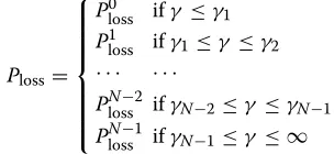
The packet loss objective function could be described as

(6)

whereqm,n is the average number of slots in state (m,n) per second. When the buffer is empty, we only send probe packets. As a result, there is only the packet overflow probability without packet corruption in the channel. In other states, packets suffer from both buffer overflow and channel corruption. minimize the total packet loss:

arg min

γ1,...,γN−1

Ploss(γ1,. . .,γN−1) (25)

This problem can be solved using any numerical opti-mization tools. In our research, we rely on Matlab to achieve the best threshold set for rate adaptation by the following methods: (i) We first sample the SNR with a step of 3 dB within the measured SNR range. (ii) We exhaus-tively take each combination of the SNR samples as the rate adaptation threshold and calculate the packet loss rate to obtain the optimal set of thresholds. (iii) The threshold search window is narrowed down to 6 dB (a range of 6 dB around the coarse-grained optimal threshold obtained in step ii as the center, based on the fact that the packet loss rate is a convex function of SNR). Then, we apply a finer-grained step (e.g. 1 dB) to the optimal threshold searching window obtained in step iii. We repeat this process till we achieve the expected SNR resolution for the thresholds.

Moreover, similar to the Matlab method, we also empir-ically search the corresponding threshold set for rate adaptation on an FPGA-based platform with repeatable controlled channel. The difference between the two meth-ods is that in Matlab, we apply the Markov model to calculate the packet loss rate. In hardware experiments, we directly measure the throughput to determine the opti-mal threshold. However, we show that the results from the two methods converge.

2.5 Rate adaptation with instantaneous buffer information

With instantaneous buffer information available for rate adaptation, the transmitter could potentially make bet-ter rate decisions by applying different channel quality thresholds according to different levels of buffer occu-pancy. Assume that the transmitter has access to the instantaneous buffer status and the channel information before each packet transmission. We continue to use the available packet space notation defined in (21). If the channel is in staten, the packet loss rate,Pn_loss, is expressed as follows:

Here, the first term is the packet overflow at the buffer, and the second term accounts for the packet corruption over the channel. minimize the total packet loss:

arg min

γ₁,...,γN−1

Ploss(γ1,. . .,γN−1) (28)

We can search the optimal threshold as shown in Figure 3. Given a buffer status, we can calculate the packet loss rate for each transmission rate over the entire range of SNR value, as in (26). Then, we plot the packet loss rate versus SNR on the same figure. We then select the crossover point between the two adjacent rates as the opti-mal threshold between the two channel states. For each value ofv, we obtain a set ofγ1toγN−1. As a result, we achieve a two-dimensional threshold matrixγv,n for the transmitter to decide which rate to use with the given channel gain and buffer status.

3 Experiment settings

The FPGA-based platform we use for our experimental evaluation is the Wireless Open-Access Research Platform (WARP). WARP is a useful wireless communication sys-tem supporting a fully customized cross-layer design [13]. WARP is used by a number of academic and industrial research labs for protocol implementation. Mainly, the physical layer implementation is in the FPGA logic fab-ric, and the higher layers exist as code on an embedded PowerPC.

(7)

−100 −5 0 5 10 15 20 25 30 35 100

200 300 400 500 600 700

SNR (dB)

Packet Loss Rate (Packet/s)

Packet Loss Rate for Rate 0 Packet Loss Rate for Rate 1

γ₁

Figure 3Illustration of process for determining the threshold between two channel states.

blocks in both the transmitter and the receiver are com-mon to any OFDM implementation. These blocks include FEC encoding, digital modulation, IFFT, and output fil-tering in the transmitter and input filfil-tering, FFT, channel estimation, equalization, digital demodulation, and FEC decoding in the receiver [19,25].

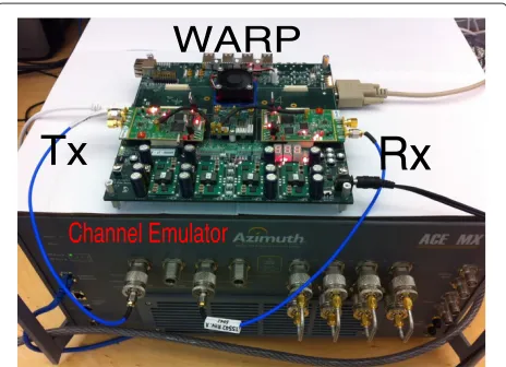
The PowerPC houses the embedded code for the MAC controller in this system. We implement the baseband processing of both the transmitter and the receiver in the same WARP board and use different daughter boards for the RF transmission and reception. As a result, we have an ideal feedback channel. However, the forward channel is time-varying and noisy, and the channel esti-mation method at the receiver is practical. We use the Azimuth ACE-MX channel emulator (Azimuth Systems, Acton, MA, USA) to generate channel effects, which can provide similar effects as complex over-the-air channels. Figure 4 illustrates the structure of our evaluation sys-tem. The equipment on the bottom is an Azimuth channel emulator and the board on the channel emulator is a WARP.

In our evaluation, we set the packet lengthL = 1, 024 B. Note that it is easy to find the optimal parame-ters for other packet lengths by following the process in Section 2. In order to cover all the SNR regions for all 8 rates, we set up a Rayleigh fading channel with an average SNR γ¯ = 15 dB and a Doppler frequency of 10 Hz. We generate the distribution of a packet source according to Poisson random process with three differ-ent average packet rates, λ ∈ {244, 977, 3906} packets

per second, corresponding to{2.0, 8.0, 32.0}Mbps, respec-tively. For easy illustration, in the analytical model, we set the buffer size to 2 and 8 packets (2,048 and 8,192 B), respectively, to examine the effect of different buffer sizes. In order to show the practical impact of this work, we also experimentally evaluated a normal buffer size of 256 packets (2 Mb) and showed the results. For a given offered load and rate adaptation scheme, we define the

throughput efficiency as the throughput with a certain threshold normalized by the throughput with the optimal threshold.

Tx

_Rx

Channel Emulator

WARP

(8)

4 Experimental results with statistical buffer information

In this section, we show how the statistical buffer infor-mation and offered load distribution affect the rate adap-tation strategy and the resulting throughput.

4.1 Experimental evaluation of rate adaptation with probe packets

In this section, we evaluate the system performance when probe packets are used. The transmitter keeps send-ing probe packets when there are no data packets in the buffer. Probe packets can provide more accurate and updated channel status information but induce additional overhead into the system.

4.1.1 Effect of diverse offered load

To demonstrate the effect of diverse offered load and buffer size, we now dynamically select the modulation and coding scheme between rate 0 and rate 4 (refer to Table 1) according to the channel status. Figure 5 shows the offered load effect when the buffer size is 2 packets. For differ-ent offered loads, the optimal rate adaptation threshold varies. For a 32-Mbps stream, the best SNR threshold is approximately 10 dB. Conversely, a 11.5-dB SNR threshold will enable the system to obtain the highest throughput when using a 8-Mbps stream. Similarly, the optimal SNR threshold for a stream of 2 Mbps is 12.5 dB. As discussed before, a system that does not consider the buffer size and buffer status will always assume a full occupancy of the buffer. In our experimental scenario, a 32-Mbps stream will predominantly keep the buffer full because the aver-age channel capacity is around 16 Mbps. However, if we do not take the offered load distribution and buffer sta-tus information into account, we would use 10-dB SNR as

the adaptation threshold. As a result, there will be about 3% throughput degradation for the 8-Mbps stream and 5% degradation for the 2-Mbps stream.

In Tables 3, 4, and 5, we list the different optimal thresh-olds for 8-rate, 4-rate, and 2-rate rate adaptations for different offered load and buffer size. We use all 8 rates in IEEE 802.11g standard for the 8-rate adaptation exper-iments. For 4-rate adaptation, we use rate 0, rate 2, rate 4, and rate 6. Rate 0 and rate 4 are used in 2-rate rate adap-tation experiments (refer to Table 1 for more information about each rate). For each threshold, the value inside the brackets is calculated from our Matlab model and the value outside is trained in hardware. We can see that by entirely different optimization methods, the thresholds converge, although there are small variations between the software model result and the hardware testing result due to the approximation in the model and the variations in hardware. We can see that for different offered load, the best rate adaption thresholds vary dramatically.

4.1.2 Effect of diverse buffer size

We examined the different optimal thresholds for differ-ent buffer sizes with the same offered load. We set the offered load to 8 Mbps in our experiments and adap-tively change the transmission rate between rate 0 and rate 4. Clearly, in Figure 6, for an 8-packet buffer, we find a different optimal adaptation threshold from the case of a 2-packet buffer. With an 8-Mbps stream, the best threshold is 12.5 dB for 8-packet buffer, while the best threshold is 11.0 dB for a 2-packet buffer. The intuitive explanation is that, compared to the 8-packet buffer, the 2-packet buffer is more likely to overflow due to the dynamic offered load and dynamic channel capacity. In order to get a balance between the overflow loss and the channel

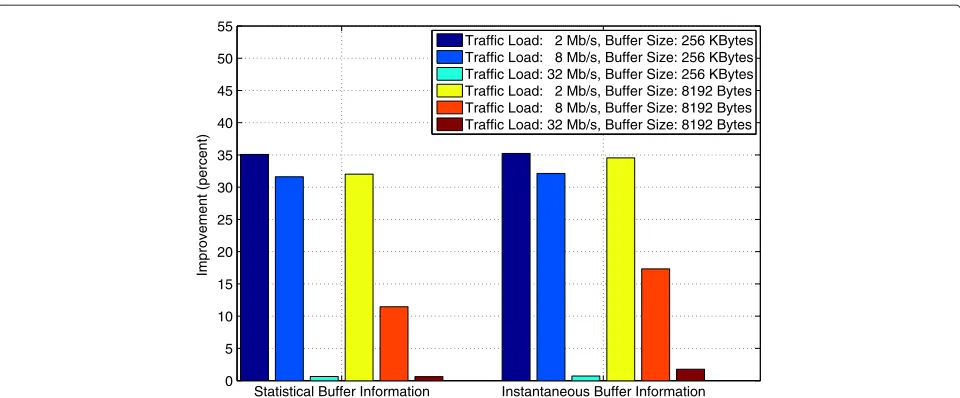
Statistical Buffer Information Instantaneous Buffer Information 0

2 4 6 8 10 12

Improvement (percent)

Traffic Load: 2 Mb/s, Buffer Size: 256 KBytes Traffic Load: 8 Mb/s, Buffer Size: 256 KBytes Traffic Load: 32 Mb/s, Buffer Size: 256 KBytes Traffic Load: 2 Mb/s, Buffer Size: 8192 Bytes Traffic Load: 8 Mb/s, Buffer Size: 8192 Bytes Traffic Load: 32 Mb/s, Buffer Size: 8192 Bytes

(9)

Table 3 The 8-rate adaptation thresholds

Offered load Buf. size (byte) Adaptation threshold (dB)

γ₁ γ₂ γ₃ γ₄ γ₅ γ₆ γ₇

2 Mbps 2,048 10.0(9.8) 11.0(11.0) 12.0(12.8) 14.0(15.0) 18.0(18.2) 20.0(21.2) 22.5(22.2)

8,192 11.0(10.4) 12.0(11.8) 14.5(13.6) 15.0(14.2) 19.0(18.2) 22.0(21.4) 23.0(22.4)

8 Mbps 2,048 6.0(5.8) 8.0(8.0) 10.0(9.2) 13.0(12.6) 16.0(14.8) 20(19.4) 22.5(21.2)

8,192 6.5(6.2) 9.0(8.4) 11.0(10.0) 14.0(13.2) 17.0(16.4) 22.0(20.2) 23.0(21.6)

32 Mbps 2,048 4.0(4.4) 5.5(5.4) 8.0(7.6) 11.5(10.8) 14.5(13.6) 19.0(18.4) 22.5(21.8)

8,192 4.5(4.4) 6.0(5.6) 8.5(8.0) 12.0(11.4) 15.0(14.0) 19.5(18.8) 23.0(22.2)

No buf./load info. 4.0(4.2) 5.3(5.2) 8.0(7.8) 11.2(10.8) 14.6(13.8) 19.3(18.6) 22.7(21.4)

The value inside the brackets is calculated from our Matlab model and the value outside is obtained using WARP.

corruption loss, the threshold should be lowered in order to transmit more packets in the channel to maximize total throughput.

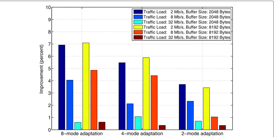
4.1.3 Performance evaluation

We evaluate buffer-information-assisted rate adaptation and show the results in Figure 7. With the consideration of other systems with different number of rate options, we consider different adaptation schemes. For 8-rate adap-tation, we use all 8 rates listed in Table 1. Rates 0, 2, 4, and 6 are used for 4-rate adaptation. Lastly, we select between rate 0 and rate 4 in 2-rate evaluation. Clearly, we can see that the improvement increases as the offered load decreases. For a packet rate of 2 Mbps, the performance may be improved as much as 7 percent with only the sta-tistical offered load and buffer information known. The improvement will be even higher for a lower offered load than 2.0 Mbps.

Table 4 The 4-rate adaptation thresholds (between rates 0, 2, 4, and 6)

Offered load Buffer size (bytes) Adaptation threshold (dB)

γ₁ γ₂ γ₃

2 Mbps 2,048 10.0(9.2) 15.0(14.6) 19.0(17.8)

8,192 12.0(10.8) 14.5(14.4) 20.0(18.2)

8 Mbps 2,048 6.5(6.2) 12.5(11.4) 19.0(17.8)

8,192 7.5(7.0) 13.5(12.8) 20.5(17.6)

32 Mbps 2,048 5.0(5.0) 10.0(9.8) 18.5(16.8)

8,192 5.0(5.2) 11.0(10.4) 19.0(17.2)

No buffer/load information

4.7(4.6) 10.5(10.0) 18.6(16.6)

The value inside the brackets is calculated from our Matlab model and the value outside is trained in hardware.

4.2 Experimental evaluation of rate adaptation without probe packets

Although probe packets can provide more accurate and updated channel status information for the transmitter to select the proper transmit rate, it costs more energy and time resources compared to the case without probe pack-ets. In this section, we evaluate the system performance, when the transmitter remains idle when there are no pack-ets in the buffer, and compare it with the system with probe packets.

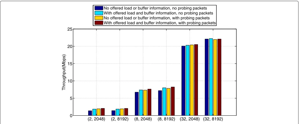
We directly compare the throughput efficiency between cases with and without probe packets enabled, as shown in Figure 8. Compared to the case with probe packets, the throughput efficiency improves more with offered load distribution and buffer information considered for the case without the probe packets. As shown in Figure 8, con-sidering offered load distribution and buffer information, instead of using 10 dB as the threshold, we will use 12

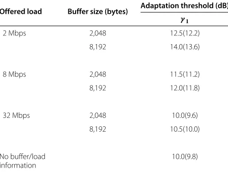
Table 5 The 2-rate adaptation thresholds (between rate 0 and rate 4)

Offered load Buffer size (bytes) Adaptation threshold (dB) γ₁

2 Mbps 2,048 12.5(12.2)

8,192 14.0(13.6)

8 Mbps 2,048 11.5(11.2)

8,192 12.0(11.8)

32 Mbps 2,048 10.0(9.6)

8,192 10.5(10.0)

No buffer/load information

10.0(9.8)

(10)

Statistical Buffer Information Instantaneous Buffer Information 0

5 10 15 20 25 30 35 40 45 50 55

Traffic Load: 2 Mb/s, Buffer Size: 256 KBytes Traffic Load: 8 Mb/s, Buffer Size: 256 KBytes Traffic Load: 32 Mb/s, Buffer Size: 256 KBytes Traffic Load: 2 Mb/s, Buffer Size: 8192 Bytes Traffic Load: 8 Mb/s, Buffer Size: 8192 Bytes Traffic Load: 32 Mb/s, Buffer Size: 8192 Bytes

Figure 6Throughput efficiency with different SNR threshold with 8-packet buffer.Throughput efficiency is defined as the throughput with a certain threshold normalized by the throughput with the optimal threshold.

dB for probing case and 20 dB for non-probing case, which results in nearly 5% and 21% throughput improve-ment for the probing and non-probing cases, respectively. Consequently, with offered load distribution and buffer information considered, there is considerable through-put compensation for the case without probe packets compared to that with probe packets.

Figure 9 shows the actual throughput improvement when probe packets are not applied in the system. The

throughput can improve as much as 35% in this case. Clearly, when channel probing is disabled, the improve-ment by exploiting offered load and buffer information is much higher than that in the case with probe packets.

5 Experimental results with instantaneous buffer information

With instantaneous buffer information, the transmitter is able to adapt the transmit rate more accurately to

−5 0 5 10 15 20 25 30

0.4 0.5 0.6 0.7 0.8 0.9 1 1.1

Adaptation SNR Threshold (dB)

Throughput Efficiency

Traffic Load: 2 Mb/s, buffer size: 2048 Byte Traffic Load: 8 Mb/s, buffer size: 2048 Byte Traffic Load: 32 Mb/s, buffer size: 2048 Byte No buffer information

(11)

−5 0 5 10 15 20 25 30 0.65

0.7 0.75 0.8 0.85 0.9 0.95 1

Adaptation SNR Threshold (dB)

Throughput Efficiency

Traffic Load: 8 Mb/s, buffer size: 2048 Byte Traffic Load: 8 Mb/s, buffer size: 8192 Byte

Figure 8Comparison of throughput efficiency of systems with and without probe packets.

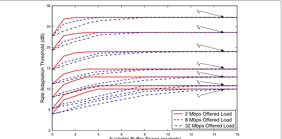
achieve a better performance. We show the different optimal rate adaptation thresholds with different offered loads and available buffer space in Figure 10. First, the rate adaptation thresholds increase with more available space in the buffer. Intuitively, the transmitter can wait for a better channel state to transmit the packet. Thus,

with more available space in the buffer, the buffer over-flow probability decreases. As a result, increasing the rate adaptation threshold to decrease the packet corruption probability in the channel leads to a better overall per-formance. Second, for the same available buffer space, when offered load is increasing, the buffer overflow rate

8−mode adaptation 4−mode adaptation 2−mode adaptation 0

1 2 3 4 5 6 7 8 9 10

Traffic Load: 2 Mb/s, Buffer Size: 2048 Bytes Traffic Load: 8 Mb/s, Buffer Size: 2048 Bytes Traffic Load: 32 Mb/s, Buffer Size: 2048 Bytes Traffic Load: 2 Mb/s, Buffer Size: 8192 Bytes Traffic Load: 8 Mb/s, Buffer Size: 8192 Bytes Traffic Load: 32 Mb/s, Buffer Size: 8192 Bytes

(12)

(2, 2048) (2, 8192) (8, 2048) (8, 8192) (32, 2048) (32, 8192) 0

5 10 15 20 25

Throughput(Mbps)

No offered load or buffer information, no probing packets With offered load and buffer information, no probing packets No offered load or buffer information, with probing packets With offered load and buffer information, with probing packets

Figure 10Rate adaptation threshold with different buffer status and offered load distributions.

increases. Then, a decrease in the rate adaptation thresh-old will result in a higher packet transmission rate, which could counteract the packet overflow rate with greater channel corruption risk to reduce packet loss. Also, we can see that when the available buffer space reaches a cer-tain value, the rate adaptation threshold converges to a constant level. In this situation, the packet corruption rate in the channel decreases to a negligible level by using a much more robust rate, and the packet overflow rate also decreases to a small value because of the large available buffer space.

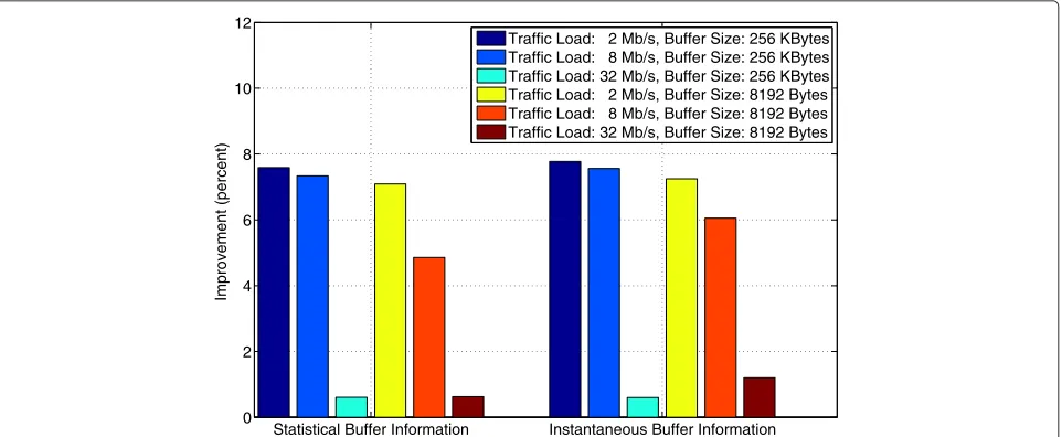
With experimental evaluation on WARP, we compare the throughput improvement between using statistical and instantaneous buffer information, with and without probe packets, as shown in Figures 11 and 12, respec-tively. We set the buffer size to 8 and 256 packets (64 Kb and 2 Mb), respectively. The transmitter adaptively select the data rate from 8 rates according to the SNR and the instantaneous buffer information. We can see that systems using instantaneous buffer information outperform those using statistical buffer information, especially when the offered load is close to the channel capacity. Note that if

8−Mode Adaptation 4−Mode Adaptation 2−Mode Adaptation 0

5 10 15 20 25 30 35 40 45

Traffic Load: 2 Mb/s, Buffer Size: 2048 Bytes Traffic Load: 8 Mb/s, Buffer Size: 2048 Bytes Traffic Load: 32 Mb/s, Buffer Size: 2048 Bytes Traffic Load: 2 Mb/s, Buffer Size: 8192 Bytes Traffic Load: 8 Mb/s, Buffer Size: 8192 Bytes Traffic Load: 32 Mb/s, Buffer Size: 8192 Bytes

(13)

0 2 4 6 8 10 12 14 16 0

5 10 15 20 25 30

Available Buffer Space (packets)

Rate Adaptation Threshold (dB)

2 Mbps Offered Load 8 Mbps Offered Load 32 Mbps Offered Load

γ₇

γ₆

γ₅

γ₄

γ₃

γ₂

γ₁

Figure 12Performance comparison between instantaneous buffer information and statistical buffer information without probe packets.

the offered load is far smaller than the channel capacity, the buffer will be empty most of the time. As a result, the instantaneous buffer information converges to the statis-tical buffer information. Similarly, if the offered load is far greater than the channel capacity, the buffer will be full most of the time. Hence, the instantaneous buffer infor-mation also converges to the statistical buffer inforinfor-mation. As a result, in these two extreme cases, instantaneous buffer information provides little benefit compared to statistical buffer information.

6 Related work

Dynamic resource allocation (e.g., transmit power and transmit rate) has been shown to be an effective solu-tion to improve system performance in wireless net-works [26,27]. Rate adaptation has been studied using loss-based and channel-quality-based mechanisms. The problem of combining finite buffer and rate adaptation has also been addressed in several papers. In [10], the authors considered a constant-frame-duration system in which the number of packets transmitted during one PHY frame is different for different transmission rates. Moreover, the authors formulated the system based on a Markov chain to reduce the packet loss rate. In [11], the authors analyzed the buffer-assisted rate adaptation problem with the constraint of a constant total power con-sumption. The authors found that in a correlated fading channel, the structure of the optimal buffer and channel adaptive transmission policies can be in sharp contrast to the water-filling strategy. The author of [12] also dis-cussed rate adaptation with transmit buffer information

in the system with partial channel information at the transmitter along with no transmitter buffer information, statistical transmit buffer information, and instantaneous transmit buffer information at the receiver, respectively. All the works above aim to maximize the total throughput with the constraint of a maximum average transmit power, which tends to add more delay to save power.

In [14], the authors relaxed the maximum average transmit power constraint and generally analyzed the procedure of buffer-assisted rate adaptation in a constant-frame-duration system, studying the packet loss rate. The complexity of this algorithm is low. However, this method cannot guarantee optimal levels of throughput. Moreover, they did not consider the idle time when there are no packets in the buffer. In contrast to that algorithm, we con-sider and analyze a variable-frame-duration system and jointly consider every threshold to directly find the set of thresholds to get the optimal throughput [28].

7 Conclusion

(14)

thresholds for systems with and without probe packets. We showed substantial improvement with the considera-tion of offered load distribuconsidera-tion and buffer informaconsidera-tion in the system.

In future work, extension to variable packet length and user scenarios could be considered. For multi-user rate adaptation, the optimization objective will be maximizing the throughput of the entire network, which requires a different strategy compared to the single-user system. Moreover, evaluation of both power and rate adaptation is challenging but important for mobile devices in the future.

Competing interests

The authors declare that they have no competing interests.

Received: 11 December 2013 Accepted: 7 April 2014 Published: 23 April 2014

References

1. JC Bicket, Bit-rate selection in wireless networks. MS Thesis, MIT, (2005) 2. S Wong, S Lu, H Yang, V Bharghavan, Robust rate adaptation for 802.11

wireless networks, inProceedings of the 12th Annual International Conference on Mobile Computing and Networking (MobiCom ‘06) (Los Angeles, CA, USA, 2006), pp. 146–157

3. M Lacage, M Hossein, T Turletti, IEEE 802.11 rate adaptation: a practical approach Master’s Thesis, (2004)

4. A Kamerman, L Monteban, WaveLAN II: a high-performance wireless LAN for the unlicensed band. Bell Labs Techn. J, 118–133 (1997)

5. Kim J, Kim S, Choi S, Qiao D, CARA: collision-aware rate adaptation for IEEE 802.11 WLANs, inProceedings of the 25th IEEE International Conference on Computer Communications (INFOCOM 2006)(Barcelona, Catalunya, Spain, 2006), pp. 1–11

6. B Sadeghi, V Kanodia, A Sabharwal, E Knightly, Opportunistic media access for multirate ad hoc networks, inProceedings of the 8th Annual International Conference on Mobile Computing and Network (MobiCom ‘02) (Atlanta, Georgia, USA, 2002), pp. 24–35

7. G Holland, N Vaidya, P Bahl, A rate-adaptive MAC protocol for multi-hop wireless networks,, inProceedings of the 7th Annual International Conference on Mobile Computing and Network (MobiCom ‘01) (Rome, Italy, 2001), pp. 236–251

8. M Vutukuru, H Balakrishnan, K Jamieson, Cross-layer wireless bit rate adaptation. SIGCOMM Comput. Commun. Rev.39(4), 3–14 (2009) 9. D Halperin, W Hu, A Sheth, D Wetherall, Predictable 802.11 packet delivery from wireless channel measurements. SIGCOMM Comput. Commun. Rev.41(4) (2010)

10. H-C Yang, S Sasankan, Analysis of channel-adaptive packet transmission over fading channels with transmit buffer management. IEEE Trans. Veh. Tech.57(1), 404–413 (2008)

11. AT Hoang, M Motani, Cross-layer adaptive transmission: optimal strategies in fading channels. IEEE Trans. Comm.56(5), 799–807 (2008) 12. D Rajan, Exploiting transmit buffer information at the receiver in

block-fading channels. EURASIP J. Adv. Signal Process.2009, 235–245 (2009)

13. J Camp, E Knightly, Modulation rate adaptation in urban and vehicular environments Cross-layer implementation and experimental evaluation. IEEE/ACM Trans. Netw.18(6), 1949–1962 (2010)

14. Q Liu, S Zhou, GB Giannakis, Queuing with adaptive modulation and coding over wireless links: cross-layer analysis and design. IEEE Trans. Wireless Comm.4(3), 1142–1153 (2005)

15. JP Tapia, J Liu, Y Karimli, M Feuerstein,HSPA Performance and Evolution: A Practical Perspective, 1st edn. (Wiley, USA, 2009)

16. HSPA. http://www.3gpp.org/technologies/keywords-acronyms/99-hspa (03/04/2014)

17. AJ Goldsmith, Chua S-G, Variable-rate variable-power MQAM for fading channels. IEEE Trans. Comm.45(10), 1218–1230 (1997)

18. AJ Goldsmith, S-G Chua, Adaptive coded modulation for fading channels. IEEE Trans. Comm.46(5), 595–602 (1998)

19. IEEE 802.11, Wireless LAN Medium Access Control (MAC) and Physical Layer (PHY) Specifications. IEEE-SA. 12 Jun 2007

20. T Karagiannis, M Molle, M Faloutsos, A Broido, A nonstationary Poisson view of internet traffic, inProceedings of the twenty-third Annual Joint Conference of the IEEE Computer and Communications Societies (INFOCOM 2004), vol. 3 (Hong Kong, 2004), pp. 1558-1569

21. A Leon-Garcia,Probability and Random Process for Electrical Engineering, 2nd edn. (Addison-Wesley, 1994)

22. GL Stuber,Principles of Mobile Communications, 2nd edn. (Kluwer, Norwell, 2000)

23. HS Wang, N Moayeri, Finite-state Markov channel-a useful model for radio communication channels. IEEE Trans. Veh. Tech.44(1), 163–171 (1995) 24. J Razavilar, KJR Liu, SI Marcus, Jointly optimized bit-rate/delay control

policy for wireless packet networks with fading channels. IEEE Trans. Comm.50(3), 484–494 (2002)

25. PO Murphy, Design, implementation and characterization of a cooperative communications system. PhD Thesis, Rice University, (2010) 26. D Lopez-Perez, X Chu, AV Vasilakos, H Claussen, On distributed and

coordinated resource allocation for interference mitigation in self-organizing LTE networks. IEEE/ACM Trans. Netw.21(4), 1145–1158 (2013)

27. D Lopez-Perez, X Chu, AV Vasilakos, H Claussen, Power minimization based resource allocation for interference mitigation in OFDMA femtocell networks. IEEE J. Sel. Area Comm.32(2), 333–344 (2014)

28. Y Du, D Rajan, J Camp, Analysis and experimental evaluation of rate adaptation with transmit buffer information, inProceedings of the 9th International Wireless Communications and Mobile Computing Conference (IWCMC 2013)(Cagliary, Sardinia, Italy, 2013), pp. 194–200

doi:10.1186/1687-1499-2014-62

Cite this article as:Duet al.:Analysis and experimental evaluation of rate adaptation with transmit buffer information.EURASIP Journal on Wireless

Communications and Networking20142014:62.