R E S E A R C H
Open Access
Stochastic bifurcation analysis in Brusselator
system with white noise
Changzhao Li
1*and Juan Zhang
2*Correspondence:
1Faculty of Civil Engineering and
Mechanics, Kunming University of Science and Technology, Kunming, China
Full list of author information is available at the end of the article
Abstract
In this paper, we mainly study the stochastic stability and stochastic bifurcation of Brusselator system with multiplicative white noise. Firstly, by a polar coordinate transformation and a stochastic averaging method, the original system is transformed into an Itô averaging diffusion system. Secondly, we apply the largest Lyapunov exponent and the singular boundary theory to analyze the stochastic local and global stability. Thirdly, by means of the properties of invariant measures, the stochastic dynamical bifurcations of stochastic averaging Itô diffusion equation associated with the original system is considered. And we investigate the phenomenological bifurcation by analyzing the associated Fokker–Planck equation. We will show that, from the view point of random dynamical systems, the noise “destroys” the
deterministic stability. Finally, an example is given to illustrate the effectiveness of our analyzing procedure.
Keywords: Stochastic bifurcation; Stochastic averaging; Largest Lyapunov exponent; Singular boundary theory; Brusselator system
1 Introduction
The determined Brusselator is a coupled differential equation written as
⎧ ⎨ ⎩
u=A– (B+ 1)u+u2v,
v=Bu–u2v, (1.1)
whereu(t) andv(t) are the concentrations of reactants at timet, respectively.A> 0 and
B> 0 are external system parameters describing the (constant) supply of “reservoir” chem-icals. As a theoretical model for a type of autocatalytic reaction, the Brusselator model has attracted the attention of many scholars since it was proposed by Prigogine and Lefever [1]. Abundant dynamical behaviors have been reported for several decades; see [2–6].
Unfortunately, it is generally recognized that the effects of “external fluctuations” (envi-ronmental noises) are inevitable in dynamical systems due to various factors, such as pos-sible changes of system parameters, variations in excitations, errors in modeling schemes. Therefore, to be more realistic, there is need to take into account stochastic systems which consider external influences in complex physical systems. There are a lot of papers about the stochastic Brusselator model. Tu and You [7] considered the existence of random
tractor. In [8], Arnold et al. performed mainly a numerical study of the bifurcation behavior of the Brusselator under parametric white noise. For other results, see [9–11].
There exist two ways to develop a stochastic model corresponding to a deterministic model to study the effect of fluctuating environment on its dynamical behavior. The first one is to replace the time independent parameters involved with the deterministic model system by some random parameters. For example, according to the orthogonal polynomial approximation in Hilbert space, Ma [12] considered the stochastic Hopf bifurcation of the following stochastic Brusselator model:
⎧ ⎨ ⎩
dx
dt = (B¯– 1)x+A
2y+Bx¯ 2
A + 2Axy+x
2y,
dy
dt = –Bx¯ –A2y–
¯
Bx2
A – 2Axy–x2y,
whereB¯is a random parameter. The obtained critical value of the stochastic Hopf bifur-cation isBc=A2+ 1 –
√ 3δ
2 .
And the second one is to add randomly fluctuating driving force directly to the deter-ministic equations without affecting any particular parameter to incorporate the effect of randomly fluctuating environment ([13,14]). This type of stochastic perturbation tech-nique to study the effect of fluctuating environment was first introduced by Beretta et al. [15] on a population model system, and Shaikhet [16] and then other researchers used it [17].
In this paper, following the second method, we assume that stochastic perturbations of the state variables around their steady-state valuesE∗(u∗,v∗) are of Gaussian white noise type which are proportional to the distances of u,vfrom their steady-state values E∗, respectively. So, in order to study the effect of environmental fluctuation, the deterministic model system (1.1) can be extended to a stochastic differential equation system as follows:
⎧ ⎨ ⎩
u= (A– (B+ 1)u+u2v) dt–δ(u–u∗) dW(t),
v= (Bu–u2v) dt+δ(v–v∗) dW(t), (1.2)
where (u∗,v∗) = (A,AB),A,Bandδare the deterministic parameters;W(t) is standard real-valued Wiener process on the complete probability space (Ω,F,P).
Therefore, in this paper, by applying the stochastic average method, singular boundary theory and invariant measure theory, we aim to analyze stochastic stability and bifurcation of system (1.2).
2 Preliminaries
For the reader’s convenience, firstly, we present the following results about singular boundary theory. To learn more about the classification of singular boundary, see [18] and [19], the reference cited therein.
According to [18] and [19], denote byxsthe boundaries of one-dimensional Itô
stochas-tic differential equation
dρ=m(ρ) dt+σ(ρ) dWρ(t).
The subscriptscan be eitherlorr, denoting the left or right boundary.
Singular Boundary of the First Kind:Consider a singular boundaryxsof the first kind,
namely, the diffusion termσ(xs) = 0. The boundary is said to be a shunt ifm(xs)= 0, and a
trap ifm(xs) = 0.
We introduce the following definitions.
(i) αsis the diffusion exponent ofxs, if
σ2(x) =O|x–xs|αs(x→xs), αs≥0.
(ii) βsis the drift exponent ofxs, if
m(x) =O|x–xs|βs(x→xs), βs≥0.
(iii) csis the drift exponent ofxs, given by
cl= lim x→x+l
2m(x)(x–xl)αl–βl
σ2(x) , cr= –xlim→x–
r
2m(x)(xr–x)αr–βr
σ2(x) .
Singular Boundary of the Second Kind:We call the boundaryxsthe singular boundary
of the second kind if the drift termm(xs) is unbounded and|xs|<∞.
(i) αsis the diffusion exponent ofxs, if
B2(x) =O|x–xs|–αs(x→xs), αs≥0.
(ii) βsis the drift exponent ofxs, if
m(x) =O|x–xs|–βs(x→xs), βs≥0.
(iii) csis the drift exponent ofxs, given by
cl= lim x→x+l
2m(x)(x–xl)βl–αl
σ2(x) , cr= –xlim→x–
r
2m(x)(xr–x)βr–αr
σ2(x) .
We also give some definitions as regards stochastic stability and bifurcation.
Definition 2.1(D-Bifurcation [18,20]) Dynamical bifurcation is concerned with a family random dynamical systems which is differential and has invariant measureμα. If there
exists a constantαD satisfying the condition in any neighborhood ofαD, there exist
an-other constantαand the corresponding invariant measureνα=μαsatisfyingνα→μαas
Definition 2.2(P-Bifurcation [18,20]) Phenomenological bifurcation is concerned with the change in the shape of stationary probability density of a family random dynamical sys-tems with the change of the parameter. If there exists a constantα0satisfying the condition
in any neighborhood ofαD, there exist two other constantsα1,α2and their corresponding
invariant measurespα1,pα2 wherepα1andpα2are not equivalent. Then the constantα0is a point of phenomenological bifurcation.
Definition 2.3(Stochastically Stable [18–20]) The trivial solutionx(t,t0,x0) of stochastic
differential equation is said to be stochastically stable or stable in probability if for every pair ofε∈(0, 1) andα> 0, there exists aδ=δ(ε,δ,t0) > 0 such that
Px(t,t0,x0)<α,∀t≥t0
≥1 –ε,
whenever|x0|<δ. Otherwise, it is said to be stochastically unstable.
Next, we will apply polar coordinate transformation and stochastic averaging method to obtain an averaging Itô diffusion equation from system (1.2).
Note that system (1.2) has the same steady-state valuesE∗(A,AB) as system (1.1). By ap-system (1.2) becomes
⎧
Hence, to analyze stochastic stability and bifurcation of system (1.2) atE∗is equivalent to consider the stochastic stability and bifurcation of system (1.2) at (0, 0).
According to the Khasminskii limiting theorem [18–20], the stochastic response process ρ(t),θ(t) of system (2.2) weakly converges to a two-dimensional Markov diffusion process. Therefore, by using the stochastic averaging method introduced in Chap. 5, Sect. 5.1 of Ref. [18], we obtain the averaged Itô stochastic differential equation for system (2.2):
⎧
whereWρ(t) andWθ(t) are independent and standard Wiener processes, the drift coeffi-cientsmi(ρ) (i= 1, 2) and the square of diffusion coefficientsσi(ρ) (i= 1, 2) are
Therefore, system (2.4) can be rewritten as ⎧
Here, we can find that the average amplitudeρ(t) is a one-dimensional Markov diffusion process. Thus, it is efficient to consider the averaging amplitude equation of system (2.5) to obtain the critical point of stochastic stability and bifurcation phenomena of system (1.2). That is, we only need to investigate the following equation:
dρ=
The essential idea of this section is to consider the stability properties of the trivial solution ρ= 0 of the stochastic model (2.6), which also addresses the asymptotical stability of the fixed pointE∗(A,BA) of system (1.2). Hereafter, we always assumeB<A2+ 1.
3.1 Local stochastic stability
calculating the largest Lyapunov exponent of the associated linearized system. We obtain the following results.
Theorem 3.1
(i) Whenδ2<A2+ 1 –B,the trivial solution of the linear Itô stochastic differential
equation(2.6)is stable in the meaning of probability,i.e.,the stochastic system(1.2)is stable at the equilibrium pointE∗.
(ii) Whenδ2>A2+ 1 –B,the trivial solution of the linear Itô stochastic differential
equation(2.6)is unstable in the meaning of probability,i.e.,the stochastic system
(1.2)is unstable at the equilibrium pointE∗.
Proof To evaluate the largest Lyapunov exponent of averaged Itô equation (2.6), we con-sider the stability of linear Itô stochastic differential equation at the trivial solutionρ= 0 first. Then one can obtain the following linearized Itô differential equation:
dρ=1
of which the solution is
ρ(t) =ρ(0)exp
so the associated largest Lyapunov exponent is
λ= lim
Based on Oseledet’s multiplicative ergodic theorem [21] (see Chap. 3 in [20] for more details), the necessary and sufficient conditions for asymptotic stability with probability one of the trivial solution of system (1.2) require that the largest Lyapunov exponent in Eq. (2.6) should be negative. Consequently, the trivial solution is locally asymptotic stable if and only ifλ< 0, i.e.,δ2<A2+ 1 –B.
This completes the proof.
3.2 Global stochastic stability
It is worth to mention that the largest Lyapunov exponent based on the multiplicative ergodic theorem is effective to estimate local stability, but it is incapable of global stability. Alternatively, we use the singular boundary theory associated with Eq. (2.6) to examine the global behaviors of the trivial solution of the system.
Generally, the boundaries of diffusion process are singular, and the boundary classifica-tion is often determined by the diffusion exponent, the drift exponent and the character value [18].
Theorem 3.2 Ifδ2<A2+ 1 –B,the trivial solution of system(2.6)is globally stable,i.e.,
Proof Asρ→0+, it is found that the asymptotic expressions for the drift termm
1(ρ) and
the square of the diffusion termσ1(ρ) are of the forms
m1(ρ) =
1 2
B–A2– 1 +3δ
2
2
ρ+O(ρ),
σ12(ρ) =δ
2ρ2
2 .
From the above equations, we know that the diffusion exponent αl (l denotes the left
boundary), drift exponentβland character valueclare, respectively,
αl= 2, βl= 1, cl= lim
ρ→0+
2m1(ρ)(ρ– 0)αl–βl
σ12(ρ) =
2(B–A2– 1 +3δ2
2 )
δ2 .
Hence, the left boundaryρ= 0 of the averaged Itô (2.6) is a trap belong to the singular boundary of the first kind. In addition, according to the classification for singular boundary in Ref. [18] (see Table 2.8-2 in Sect. 2.8.2 for details), we know that the left boundary ρ= 0 is repulsively natural if cl> 1, i.e.,δ2>A2+ 1 –B, a strictly natural ifcl= 1, i.e.,
δ2=A2+ 1 –B, and an attractively natural ifc
l< 1, i.e.,δ2<A2+ 1 –B.
Similarly, for the right boundaryρ→+∞, it is found that the asymptotic expressions for the drift termm1(ρ) and the square of the diffusion termσ1(ρ) are of the forms
m1(ρ) = –
1 8ρ
3, σ2 1(ρ) =
δ2ρ2
2 .
So, it is a singular boundary of the second kind. Accordingly, the diffusion exponentαr
(rdenotes the right boundary), the drift exponentβrand character valuecrfor the right
boundaryρ→+∞are, respectively,
αr= 2, βr= 3, cr= – lim
ρ→+∞
2m1(ρ)ραr–βr
σ12(ρ) =
1 2δ2 > 0,
i.e., for anyδ> 0,cr> –1. According to the classification for singular boundary in [18] (see
Table 2.8-4 in Sect. 2.8.2 for details), we know the right boundaryρ= +∞is a repulsively natural. Therefore, ifδ2<A2+ 1 –B, the boundaryρ= 0 is attractively natural and the
boundaryρ= +∞is exclusively natural. All solution curves enter the inner system from the right boundary and will be attracted by the left boundary, which implies that the trivial solution of system (2.6) is globally stable, i.e., the stochastic system (1.2) is globally stable at the equilibrium point.
This completes the proof.
Remark3.1 Note that ifδ2<A2+ 1 –Bholds, the stochastic system (1.2) is not only locally
but also globally stable at the equilibrium point. And the high-order-term coefficients of the drift term have no effects on the global stability of the trivial solution.
4 Stochastic bifurcation
4.1 Stochastic D-bifurcation
In this subsection, similar to the discussions in [20,22], we will prove that the stochastic system (2.6) undergoes a D-bifurcation whenδ2=A2+ 1 –B. One can see Example 4.2.15 in [20] for detailed introductions.
Supposevt= (18)
1
2ρ, we rewrite system (2.6) as
dvt=
1 2
B–A2– 1 +3δ
2
2
vt–v3t
dt+
δ2
2 1
2
vtdWr(t),
which is equivalent to the following Stratonovich stochastic differential equation:
dvt=
αvt–v3t
dt+vt◦dW(t), (4.1)
whereα=B–A22–1+δ2,= (δ22)12. As is well known, (4.1) is solved by
v→ψα(t,ω)v=
vexp(αt+Wt(ω))
(1 + 2v2t
0exp[2(αs+Ws(ω))] ds)
1 2
, (4.2)
wherevis the initial value ofvt. We now determine the domainDα(t,ω), whereDα(t,ω) :=
{φ∈R|(t,ω,φ)∈D} ⊂X(D= R×Ω×X) is the (in general possibly empty) set of initial valuesv∈Rfor which the trajectories still exist at timetand the rangeRα(t,ω) ofψα(t,ω) : Dα(t,ω)→Rα(t,ω).
We obtain
Dα(t,ω) = ⎧ ⎨ ⎩
R, t≥0;
(–dα(t,ω),dα(t,ω)), t< 0.
Here
dα(t,ω) = 1
(2|0texp(2αs+ 2Ws(ω)) ds|)
1 2
> 0
and
Rα(t,ω) =Dα–t,υ(t)ω= ⎧ ⎨ ⎩
(–rα(t,ω),rα(t,ω)), t> 0;
R, t≤0,
where
rα(t,ω) =dα–t,υ(t)ω= exp(αt+Wt(ω)) (2|0texp(2(αs+Ws(ω))) ds|)
1 2
> 0.
We can now determine
Eα(ω) :=
and obtain
The ergodic invariant measures are
• forα≤0, the only invariant measures isμα
1,ω=δ0,
• forα> 0, we have the three invariant forward Markov measuresμα
1,ω=δ0,
μα2,ω=δ–d–
α(ω)andμ
α
3,ω=δd–
α(ω); the functions are the solutions of the corresponding
Fokker–Planck equations (FPK).
Next, we will calculate the Lyapunov exponent for each of these measures. The linearized random dynamical system (RDS)φt=Dψα(t,ω,v)φis as follows:
on the condition that the integrability condition (IC)v2∈L1(P) is satisfied.
Therefore, we conclude to the following.
(i) Forα∈R, the IC forμα1,ω=δ0is trivially satisfied and we have
of which the unique probability density solution is
Since
Eμα
2,ωv
2= E–dα
–
2
=
∞
0
v2p2(v) dv<∞,
the IC is satisfied. The calculation of the Lyapunov exponent is accomplished by observing that
d–α(υtω)
2
= exp(2αt+ 2Wt(ω))
2–∞t exp(2αs+ 2Ws(ω)) ds
= Ψ
(t)
2Ψ(t),
where
Ψ(t) =
t
–∞
exp2αs+ 2Ws(ω)
ds.
Then by the ergodic theorem
Ed–α2=1 2tlim→∞
1
tlogΨ(t) =α,
therefore,
λμα2,ω= –2α< 0,
which implies the invariant measureμα
2,ωis stable forα> 0.
(iii) Forα> 0,μα
3,ω=δd–
α(ω)isF
0
–∞measurable and because of its probability density
p3(v)is equal top2(v),
E–dα– 2
= Ed–α 2
=α,
thenλ(μα
3,ω) =λ(μ α
2,ω) = –2α< 0. Likewise, we conclude that the invariant measure
μα3,ωis stable forα> 0.
Hence, the following result is obvious.
Theorem 4.1 Ifα< 0,i.e.,δ2<A2+ 1 –B,the RDSψ
α(t,ω)possesses exactly one invariant measureμα1,ω,which is stable.Ifα> 0,i.e.,δ2>A2+ 1 –B,the RDSψ
α(t,ω)possesses three
random Dirac measuresμα1,ω,μ2,αω,μα2,ω,whereμα1,ωis unstable,whileμα2,ωandμα3,ωare stable.Therefore,the RDSψα(t,ω)undergoes a D-bifurcation at the pointαD= 0,i.e.,the
stochastic system(2.6)undergoes a stochastic pitchfork bifurcation(for more details,see
[20])whenδ2passes through A2+ 1 –B.
Remark4.1 Note that ifδ= 0,αD= 0 is equivalent toB=A2+ 1, which is just the critical
condition for the Hopf bifurcation of the determined system (1.1).
4.2 Stochastic P-bifurcation
Namachivaya’s theory ([20,23]), the extreme value ofPst(ρ) gives essential information on
the stationary behavior of the Fokker–Planck equation arising from nonlinear stochastic systems.
More specifically, ifPst(ρ) has a maximum value atρ∗, the sample trajectory will stay
for a longer time in the neighborhood ofρ∗, i.e.,ρ∗is stable in the meaning of probability (with a bigger probability). IfPst(ρ) has a minimum value (zero), it is just the opposite.
Notice that the averaged FPK equation associated with Eq. (2.6) is
∂P(ρ)
whereP(ρ) is the probability density of diffusion processρ(t) and the stationary probabil-ity densprobabil-ityPst(ρ) satisfies the following degenerate equation:
0 = – ∂
For the above equation, its exact stationary solutionPst(ρ) can be expressed as follows:
Pst(ρ) =Cρ
To obtain the extreme value point of the probability densityPst(ρ), we need to solve
dPst(ρ)
For the roots of Eq. (4.3), there are three cases to discuss.
(i) Ifδ2< 2(A2+ 1 –B), for Eq. (4.3), there are no real roots. The probability density
functionPst(ρ)tends to infinite asρ→0+. In this case, the random trajectories of
system (2.6) are concentrated in a neighborhood of the pointρ= 0. (ii) Whenδ2= 2(A2+ 1 –B), for (4.3), there is only one root,ρ= 0, for which
i.e., the probability density functionPst(ρ)possesses the maximum value at the
i.e.,Pst(ρ)possesses a maximum value at the pointρ=ρ∗. Meantime,Pst(ρ)attains
the minimum value at the pointρ= 0, but the derivative ofPst(ρ)does not exist at
the pointρ= 0. In this case, the random trajectories of system (2.6) are concentrated in a neighborhood of the pointρ=ρ∗.
Therefore, we obtain the following result.
Theorem 4.2 If A2+ 1 –B> 0,Eq. (2.6)undergoes stochastic P-bifurcations when the
pa-rameterδ=2(A2+ 1 –B),i.e.,system(1.2)undergoes phenomenological bifurcations at
the critical parameter valueδ=2(A2+ 1 –B).
5 Numerical simulations
In this section, we consider an illustrative numerical example to verify the analytic results obtained above.
Example5.1 For (2.6), the values of the parameters in simulations are chosen as follows:
A= 1,B= 1.88. In this case,A2+ 1 –B= 0.12 > 0. Following the discussion in Sect.4.2, we
have stationary probability density function
Pst(ρ) =
ρδ 2–0.24
δ2 e– ρ2
4δ2
Γ(δ2–0.12 δ2 )[(2δ)
2(δ2–0.12)
δ2 ]
,
and by solving dPst(ρ)
dρ = 0, we need to solve
ρ–0.24δ2 ρ2– 2δ2– 0.24= 0. (5.1)
Hence, we have the following.
Case1. Whenδ2 < 0.24, Eq. (5.1) has no real roots. The probability density function
Pst(ρ)tends to infinity asρ→0+. In this case, the random trajectories of system
(2.6) are concentrated in a neighborhood of the pointρ= 0. See Fig.1.
Figure 1Portraits ofPst(ρ) whenA= 1,B= 1.88,δ
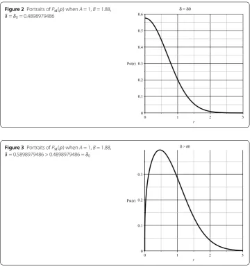
Figure 2Portraits ofPst(ρ) whenA= 1,B= 1.88,
δ=δ0= 0.4898979486
Figure 3Portraits ofPst(ρ) whenA= 1,B= 1.88,
δ= 0.5898979486 > 0.4898979486 =δ0
Case2. Whenδ2= 0.24, Eq. (5.1) has only one rootρ= 0. And
d2P st(ρ)
dρ2
ρ=0
< 0,
the probability density functionPst(ρ)becomes smooth and possesses the maximum
value at the pointρ= 0. See Fig.2, for details.
Case3. Whenδ2> 0.24, there is one positive rootρ=ρ∗= 0.4647140841of (5.1).Pst(ρ)
possesses a maximum value at the pointρ=ρ∗. In the meantime,Pst(ρ)attains the
minimum value at the pointρ= 0, but the derivative ofPst(ρ)does not exist at the
pointρ= 0. In this case, the random trajectories of system (2.6) are concentrated in a neighborhood of the pointρ=ρ∗. See Fig.3.
Therefore, we find the critical point
δ0=
2A2+ 1 –B= 0.4898979486.
Finally, we investigate the dynamics of system (1.2). We mainly consider the joint prob-ability density(x,y) to Cartesian coordinatesxandy. By the relation(x,y) =|J|(ρ,θ) andP(r) =
π
2 –π
2 (ρ,θ) dθ, where the determinant of the Jacobian matrixJof the nonlinear
transformation is given by|J|= 1ρ and is the joint probability density toρandθ (see [24]), we obtain
(x,y) = (x
2+y2)δ2–0.242δ2 e–
x2+y2
4δ2
π Γ(δ2–0.12δ2 )[(2δ) 2(δ2–0.12)
δ2 ]
.
By similar discussions, we can draw the following conclusions.
Case1. Whenδ2< 0.24, the joint probability density function(x,y)tends to infinite as
x→0andy→0. The result is shown in Fig.4.
Case2. Whenδ2= 0.24, a maximum value appears at the pointO(0, 0). See Fig.5for details.
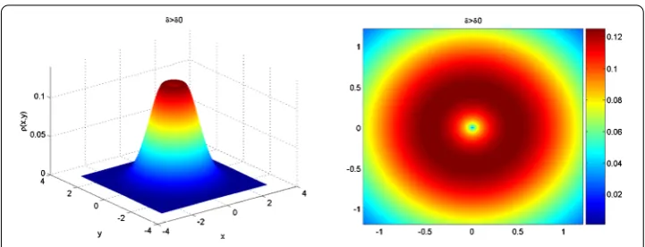
Case3. Whenδ2> 0.24, a maximum value appears at the points of stable limit cycle
x2 +y2= 0.4319183600, and a minimum value arises at the pointO(0, 0). In the
meantime, we notice that the partial derivatives of joint probability density(x,y)
are discontinuous at the original pointO(0, 0). See Fig.6.
Figure 4Portraits of(x,y) (left) and distribution of invariant densities (right) whenA= 1,B= 1.88,
δ= 0.3898979486 < 0.4898979486 =δ0
Figure 5Portraits of(x,y) (left) and distribution of invariant densities (right) whenA= 1,B= 1.88,
Figure 6Portraits of(x,y) (left) and distribution of invariant densities (right) whenA= 1,B= 1.88,
δ= 0.5898979486 > 0.4898979486 =δ0
Therefore, we find the critical point
δ0=
2A2+ 1 –B= 0.4898979486.
As a result, we conclude that Eq. (1.2) undergoes a stochastic phenomenological bifurca-tion atδ=δ0.
6 Conclusions
In this paper, by applying the stochastic average method, singular boundary theory and invariant measure theory, we study the stochastic stability and stochastic bifurcation of the Brusselator system with multiplicative white noise. Finally, an example is given to illustrate the effectiveness of our analyzing procedure.
Throughout the paper, we always assume thatB<A2+ 1. In this case, as is well known, the deterministic system (1.1) is stable. But for the stochastic case, system (1.2) undergoes stochastic D-bifurcation whenδ=√A2+ 1 –Band the stochastic P-bifurcation occurs if
δ=2(A2+ 1 –B). Therefore, we conclude that the noise will destabilize the system under
some condition.
Furthermore, we find that, for some small noise whenδ<√A2+ 1 –B, system (1.2) is
globally stable. We conclude that the small noise cannot affect the dynamical behaviors of system (1.2).
However, to the best of our knowledge, most of the existing results as regards the stochastic bifurcation analysis are mainly reported for the lower-dimensional stochastic models, especially one- or two-dimensional ones (see [24]). There are very few results about the high-dimensional stochastic systems because of the difficulty of the model re-duction of high-dimensional ones. Moreover, besides the noise effects, many other factors such as time delays and impulsive input may affect the dynamical behaviors of the models. These factors we will consider in the future.
Acknowledgements
The authors are grateful to anonymous referees for their constructive comments and suggestions which have greatly improved this paper.
Funding
Competing interests
The authors declare that they have no competing interests.
Authors’ contributions
The authors contributed equally and significantly in writing this article. Both authors read and approved the final manuscript.
Author details
1Faculty of Civil Engineering and Mechanics, Kunming University of Science and Technology, Kunming, China.2Faculty of
Science and Technology, Kunming University of Science and Technology Oxbridge College, Kunming, China.
Publisher’s Note
Springer Nature remains neutral with regard to jurisdictional claims in published maps and institutional affiliations.
Received: 14 March 2019 Accepted: 9 August 2019
References
1. Prigogine, L., Lefever, R.: Symmetry-breaking instabilities in dissipative systems. J. Chem. Phys.48, 1695–1700 (1968) 2. Li, B., Wang, M.X.: Diffusion-driven instability and Hopf bifurcation in Brusselator system. Appl. Math. Mech.29(6),
825–831 (2008)
3. Zuo, W., Wei, J.: Multiple bifurcations and spatiotemporal patterns for a coupled two-cell Brusselator model. Dyn. Partial Differ. Equ.8(4), 363–384 (2011)
4. Brown, K.J., Davidson, F.A.: Global bifurcation in the Brusselator system. Nonlinear Anal.24, 1713–1725 (1995) 5. Yu, P., Gumel, A.B.: Bifurcation and stability analysis for a couple Brusselator model. J. Sound Vib.244, 795–820 (2001) 6. Li, X.H., Hou, J.Y., Shen, Y.J.: Slow-fast effect and generation mechanism of brusselator based on coordinate
transformation. Open Phys.14(1), 261–268 (2016)
7. Tu, J.Y., You, Y.C.: Random attractor of stochastic Brusselator system with multiplicative noise. Discrete Contin. Dyn. Syst., Ser. A36(5), 2757–2779 (2016)
8. Arnold, L., Bleckert, G., Schenk-Hoppé, K.R.: The stochastic brusselator: parametric noise destroys Hopf bifurcation. In: Stochastic Dynamics, pp. 71–92. Springer, New-York (1999)
9. Xu, Y., Ma, S.J., Zhang, H.Q.: The stability analysis in stochastic Brusselator system with random parameter. Sci. Sin. Phys. Mech. Astron.41(10), 1203–1209 (2011)
10. Tambe, S.S., Inamdar, S.R., Kulkarni, B.D.: Diffusive broadening of limit cycle in presence of noise: a case study of reversible Brusselator. Math. Comput. Simul.39, 115–124 (1995)
11. Bashkirtseva, I.A., Ryashko, L.B.: Sensitivity analysis of the stochastically and periodically forced Brusselator. Physica A
278, 126–139 (2000)
12. Ma, S.J.: The stochastic Hopf bifurcation analysis in Brusselator system with random parameter. Appl. Math. Comput.
219, 306–319 (2012)
13. Bandyopadhyay, M., Chattopadhyay, J.: Ratio-dependent predator–prey model: effect of environmental fluctuation and stability. Nonlinearity18, 913–936 (2005)
14. Bandyopadhyay, M., Chakrabarti, C.G.: Deterministic and stochastic analysis of a nonlinear preypredator system. J. Biol. Syst.11, 161–172 (2003)
15. Beretta, E., Kolmanovskii, V., Shaikhet, L.: Stability of epidemic model with time delays influenced by stochastic perturbations. Math. Comput. Simul.45, 269–277 (1998)
16. Shaikhet, L.: Stability of predator–prey model after effect by stochastic perturbations. Stab. Control: Theory Appl.1(1), 3–13 (1998)
17. Saha, T., Chakrabarti, C.: Stochastic analysis of prey–predator model with stage structure for prey. J. Appl. Math. Comput.35, 195–209 (2011)
18. Zhu, W.Q.: Nonlinear Stochastic Dynamics and Control: Framework of Hamiltonian Theory. Science Press, Beijing (2003)
19. Lin, Y.K., Cai, G.Q.: Probabilistic Structural Dynamics, Advanced Theory and Applications. McGraw-Hill, New York (2004)
20. Arnold, L.: Random Dynamical Systems. Springer, New York (1998)
21. Oseledets, V.I.: A multiplicative ergodic theorem. Lyapunov characteristic numbers for dynamical systems. Trans. Mosc. Math. Soc.19, 197–231 (1968)
22. Huang, Z.T., Yang, Q.G., Cao, J.F.: Stochastic stability and bifurcation for the chronic state in Marchuk’s model with noise. Appl. Math. Model.35, 5842–5855 (2011)
23. Sri Namachchivaya, N.: Stochastic bifurcation. Appl. Math. Comput.38(2), 101–159 (1990)