Algorithms and Hardness
Thesis by
Euiwoong Lee
In Partial Fulfillment of the Requirements for the Degree of
Master of Science
California Institute of Technology Pasadena, California
c
2012
Acknowledgements
Abstract
We study a generalization of the famous k-center problem where each object is an affine subspace of dimension ∆, and give either the first or significantly improved algorithms and hardness results for many combinations of parameters. This generalization from points (∆ = 0) is motivated by the analysis of incomplete data, a pervasive challenge in statistics: incomplete data objects in Rd
can be modeled as affine subspaces. We give three algorithmic results for different values of k, under the assumption that all subspaces are axis-parallel, the main case of interest because of the correspondence to missing entries in data tables.
1) k= 1: Two polynomial time approximation schemes which runs inpoly(∆,1/)nd. 2) k= 2: O(∆1/4)-approximation algorithm which runs inpoly(n, d,∆)
3) Generalk: Polynomial time approximation scheme which runs in 2O(∆klogk(1+1/2))nd We also prove nearly matching hardness results; in both the general (not necessarily axis-parallel) case (for k ≥ 2) and in the axis-parallel case (for k ≥ 3), the running time of an approximation algorithm with any approximation ratio cannot be polynomial in even one of k and ∆, unless P = NP. Furthermore, assuming that the 3-SAT problem cannot be solved subexponentially, the dependence on both k and ∆ must be exponential in the general case (in the axis-parallel case, only the dependence on k drops to 2Ω(√k)). The simplicity of the first and the third algorithm
Contents
Acknowledgements iii
Abstract iv
1 Introduction 1
1.1 Related Work . . . 3 1.2 Our Results . . . 4
2 Preliminaries 6
3 Two algorithms for 1-center for axis-parallel flats 8
4 Clustering Hardness 16
5 Clustering Algorithms 24
6 2-Clustering of axis-parallel flats 27
7 Conclusions and Future Work 31
Chapter 1
Introduction
Clustering is one of the most important problems in computational theory. Due to its wide range of applications, it has been investigated for decades and continues to be actively studied not only in theoretical computer science, but in other disciplines such as statistics, data mining and machine learning. Generally speaking, the goal of clustering is to partition a given set of n data objects intok groups so that the objects within each group are similar. One way to represent data objects and measure similarity is to regard each data object with d features as a point in the Euclidean space Rd, where each coordinate corresponds to each feature; two objects are similar when the
Euclidean distance between them is small. Based on this observation, the famousk-means clustering (minimizing the sum of the squared distance from each point to the nearest center), k-median clustering (minimizing the sum of the distances), andk-center clustering (minimizing the maximum distance) problems have been suggested and studied both theoretically and practically.
However, in reality, data objects often do not come fully equipped with a mapping into Euclidean space. A simple and ubiquitous example can be found in a questionnaire where a few questions are left blank. Likewise, in a longitudinal medical study, a patient’s missed appointment creates missing real-valued entries in their record.
Assume that the answers to these unanswered questions, or unmeasured values, actually exist (but are not known to us). Then a “true” data point exists, and lies on the axis-parallel affine subspace fixed by the answers or measurements which wedopossess. No more information, however, can be retrieved from the incomplete data object.
heuristics. They include substituting with the sample mean and replacing a missing element using a learning algorithm or criterion (EM, max likelihood). While these methods work better than the simple deletion methods in practice [1], little is known about their theoretical performance, except in the very special and almost-never–satisfied case that the data is “missing at random”—with no correlation with the underlying missing entries. It is unusual that the experimenter even has any good probabilistic model for the “missingness” of entries, and the absence of such a model precludes guarantees of the type one is accustomed to for statistical procedures in the theoretical statistics literature.
As an alternative, Gao et al. [13] first suggested a new approach rooted in the geometry of a data set. A data object that is lacking information about one or more features corresponds to an affine subspace, also known as a flat, in Rd, whose dimension is the number of missing features.
Since the distance between a flat and a point (we still model each center as a point) is well-defined, the classical clustering problems such ask-means,k-median, and k-center can be defined on a set of flats; we simply need to find kcenters to minimize the objective function, based on the distance between each flat to its nearest center. This approach has the strong theoretical guarantee that if we find the optimal clustering of a set of flats with respect to some objective, we automatically compute the set of points, one in each flat, such that it minimizes the objective over all such sets of points. In terms of clustering incomplete data, this method computes the best guess about incomplete entries (i.e., guess about a true point in each flat) that gives the most-clusterable complete data among all guesses. Therefore, if the set of data objects is guaranteed to be well-clustered, this geometric approach yields the correct clustering as well as the correct guesses for missing entries.
1.1
Related Work
Different clustering problems have been studied extensively. Thek-median problem has been often studied in a finite metric space, where the problem can be solved exactly in polynomial time if k is fixed. For general k, there is a known (1 + 2/e)-hardness of approximation result [21] and substantial work on approximation algorithms [18, 7, 2, 21, 9], with the best guarantee a 3 + approximation. The k-means problem has been often studied in the Euclidean space, and even 2-means problem was shown to be NP-hard [8]. Instead, many PTAS’s have been suggested for the Euclideank-means and k-median problem, with the best running time polynomial in nand d but exponential ink[25, 26, 6, 9, 19, 23, 10]. Recently, the focus has been on the well-clusterable
or stable instances and approximation schemes with better running times have been suggested for those instances[27, 4, 3, 22].
The k-center problem has relatively simple history where a simple 2-approximation algorithm and an almost matching hardness result were provided for general k[17, 11]. As in the Euclidean k-means and k-median, there is a PTAS which runs in time exponential in k [6]. However, while the 1-mean problem in the Euclidean space and the 1-median problem in a finite metric space can be solved trivially, the 1-center problem in the Euclidean space, which tries to find the smallest ball containing all data points, is nontrivial. There are several approximation schemes for this 1-center problem, also known as the Minimum Enclosing Ball problem [5, 29, 28], with the best running time O(nd
) to find an enclosing ball of radius at most (1 +) times the optimal radius.
In [13], Gao et al. first suggested the problem of clustering flats as a means to cope with incomplete data, and studied the 1-center problem. They proved the existence of a −core set of size O(∆4); there is a subset of O(∆4) flats of which the optimal radius is at least 1+1 of the optimal radius of the entire set. Their main result is based on anIntrinsic-dimension Helly theorem, which says that there is a 1-core set of size ∆ + 2. However, their algorithm to find such a core set requires time exponential in ∆, so they suggested two alternative algorithms for the problem. The first algorithm using convex programming requires time ˜O(√n(d3+d2n)poly(∆)) to get a constant additive approximation, and the second algorithm using LP-type programming requires expected time O(n(poly(∆)d+ 2poly(∆))) to get a constant multiplicative approximation. In the subsequent
1.2
Our Results
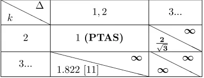
We present the algorithms and hardness results for clustering flats for many possible combinations ofkand ∆, where each of them either is the first result or significantly improves the previous results for the given values forkand ∆. Our algorithms and hardness results are summarized in Table 1.1 and 1.2 respectively. They can be classified into three categories.
1) Improved algorithms for k= 1 and the first algorithm for generalk: In Section 3, we revisit the casek= 1 where all flats are axis-parallel and suggest two PTAS’s; both are simple to describe but their running times are linear in n and d, which are even better than the fastest known algorithm, which uses a convex programming solver. We also partially explain why the problem gets harder as ∆ increases. The key lemma to many 1-center algorithms, which shows an upper bound on the distance between any point and the optimal center in terms of the radius of the minimum intersecting ball centered at that point, gets relaxed as ∆ increases. Extending one of these algorithms, in Section 5, we present a PTAS for fixedkand ∆ for the axis-parallel case. The running time to get a (1 +)-approximation is 2O(∆klogk(1+12))nd, which is tight in the sense that
it is exponential in bothkand ∆ but linear in bothnandd.
2) The first and almost matching lower bounds on approximation ratio and running
time: In Section 4, we show that actualk-center clustering(k≥2) is greatly harder than finding the minimum intersecting ball. In fact, we show that the running time of any approximation algorithm has to depend exponentially on both k and ∆; for fixed k ≥2 there is no polynomial (in n, d,∆) time algorithm that guarantees any approximation ratio, and for fixed ∆≥1 there is no polynomial (in n, d, k) time approximation algorithm either. In the axis-parallel case, the same result holds fork ≥3 and ∆≥3, meaning that the axis-parallel case is not much easier than the general case whenk and ∆ become large. Furthermore, assuming that the 3-SAT problem cannot be solved in subexponential time, our reductions also show that there cannot be any approximation algorithm for the general case whose running time is subexponential in eitherk or ∆; our algorithm is almost tight in each parameter.
3) Axis-parallel vs General, Connection to Graph Coloring, and New Helly-type
theorem Finally, in Section 6, we study axis-parallel 2-center, where our inapproximability ratio drops from∞in the general case to √2
3. The fact that axis-parallel 2-center is greatly easier than
an example where the optimal radius is Ω(d14r).
H H
H H
H k
∆
1 2...
1 (R
∗+δ, O(√n(d3+d2n)poly(∆) log (n/δ))) [13]
((1+)R∗,O(nd∆2 log
∆
))
2 ((1 +)R∗, O(ndlog 1/+nlognlog 1/)) [14] (O(∆1/4)R∗,O(dn2logn)) 3 ((1 +)R∗, O(ndlog 1/+nlog2nlog 1/)) [14] ((1+)R∗,2O(∆(1+1/2))nd)
[image:10.612.115.537.98.187.2]4... ((1+)R∗,2O(klogk(1+1/2))nd) ((1+)R∗,2O(∆klogk(1+1/2))nd) Table 1.1: Algorithms for differentkand ∆. Each pair (x, y) indicates that it takes timeyuntil the objective is less thanx, whenR∗ denotes the optimum. Prior work is indicated by plain text and a citation, and applies to general flats; results of this paper are indicated by boldface, and apply to axis-parallel flats. Algorithms in column 2...work for any value of ∆, and algorithms in row 4... work for any value ofk.
H H
H H
H k
∆
1,2 3...
2 1(PTAS) HH
H H
HH 2
√
3 ∞
3... XXXXXX XX
XX 1.822 [11]
∞ H H
H H
H ∞
∞
[image:10.612.225.424.291.367.2]Chapter 2
Preliminaries
A ∆-flat in Rd(d > ∆) is a ∆-dimensional affine space. LetL={l1, ..., ln} be the set of flats that
we want to cluster. For simplicity, we consider the situation where all of them are of dimension ∆. All our algorithms and analyses work even when Lcontains flats of different dimensions and ∆ is taken to be the greatest dimension of any flat.
For c ∈ Rd and r ∈ R+, let Bc,r be the closed ball of radius r centered at c. The ball Bc,r
intersectsLif it intersects each flat inL. LetR∗(L) be the minimum radius of any intersecting ball ofL. A minimum intersecting ball is Bc,R∗ for some c∈Rd that intersectsL. Unlike the situation
where L consists of points, there can be more than one minimum intersecting ball. LetC∗(L) be the set of points such thatc∈C∗(L) if and only ifcis the center of a minimum intersecting ball of
L. When it is clear from the context, we do not useLin these notations.
Letd(p, q) be the Euclidean distance between two pointspandq,d(p, l) = minq∈ld(p, q) be the
distance between a point p and a set of points l, and R(c,L) = maxli∈Ld(c, li) be the minimum radius of any intersecting ball centered at c. Note that R∗ ≤R(c) for allc ∈Rd. For a flatli and
its translation l0
i that contains the origin(i.e., li0 is a subspace of Rd), letdli(p, q) be the length of the vector p−q projected to l0i, and dl⊥
i (p, q) be the length of the vector p−q projected to the orthogonal complement ofl0i. By the Pythagorean theorem, (d(p, q))2= (d
li(p, q))
2+ (d
l⊥
i(p, q))
2.
Sometimes we consider the situation where all flats are axis-parallel. In this case, each flat li
is represented asli =(x1, ..., xd)|(xj1, ..., xj∆)∈R
∆ where eachx
u(u /∈ {j1, ..., j∆}) is fixed. We
sometimes writeli as a d-dimensional vector, writing∼in thejth coordinate when it is not fixed.
For example,lj = (∼,5,∼,3,1) =(x1,5, x3,3,1)|(x1, x3)∈R2 represents a 2-flat that is parallel to the first and third unit vector. Calljth coordinate trivial when there is no flat that has the fixed jth coordinate. We can assume that no coordinate is trivial since otherwise simply removing this coordinate from all flats will decrease ∆ anddby 1 while not affecting the clustering cost for any k. Letmj andMj be the minimum and the maximum of thejth coordinate over all flats that have
the fixedjth coordinate, respectively. Since the diameter of the minimum intersecting ball must be at least the largest difference in thejth coordinate for any j,R∗(L)≥maxj
Mj−mj
when the jth coordinate of c is outside of [mj, Mj] (say cj < mj), changing cj to mj does not
increased(c, li) for any li, which means that there is an optimal centerc∗ ∈ C∗ in the hypercube
[m1, M1]×...×[md, Md]. Therefore, any pointc in this hypercube satisfiesR(c,L)≤2 √
Chapter 3
Two algorithms for 1-center for
axis-parallel flats
We give two approximation schemes for the case k = 1, which is finding the smallest ball that intersects every flat. The first algorithm resembles Lloyd’s method for thek-means problem [24]; in each iteration we find the closest point to the current center in each flat, and move the current center to minimize the maximum distance to these points. However, unlike Lloyd’s method fork >1, the convergence time of this iterative method to the global optimum can be shown to be fast, as we shown in Theorem 3.1. First, we take the initial center to be any point inli∩([m1, M1]×...×[md, Md]) for
anyi. For any optimal centerc∗ in the hypercube,dl⊥
i (c, c
∗)≤d
l⊥
i (c, li) +dl⊥i (li, c
∗)≤0 +R∗≤R∗
andd2
li(c, c
∗)≤∆·max
j(Mj−mj)2≤∆·4(R∗)2. Therefore, (d(c, c∗))2≤O(∆(R∗)2) andR(c)≤
O(∆(R∗)2).
Algorithm 1Lloyd-Type Algorithm
Given a set of ∆-flats L = {l1, ..., ln} and the initial center c ∈ l1 ∩ ([m1, M1] × ... ×
[md, Md])
1: Fori= 1, ..., n, findpi∈liwhich is closer tocthan any other point inli (i.e. pi is the projection
ofc toli).
2: Find an approximate minimum enclosing ball for p1, ..., pn using an existing algorithm (see
Section 1.1). Update cto be the center of the minimum enclosing ball.
3: Iterate 1 and 2 for the precomputed number of iterations.
The convergence of Algorithm 1 depends on how fast R(c,L) is improved in each iteration. Given c and its projections p1, ..., pn to l1, ..., ln respectively, we show that there exists c0 such
that R(c0,{p1, ..., pn}) is significantly less thanR(c,{p1, ..., pn}) = R(c,L). Since in each step an
(approximate) minimum enclosing ball of{p1, ..., pn} is found, we are guaranteed that our updated
center reduces R(c,L) significantly, leading to the convergence of the algorithm. This c0 is found from the line segment joining the current centercand one of the optimal centersc∗∈C∗.
Theorem 3.1. If all flats are axis-parallel, Algorithm 1 satisfiesR(1−0)< R∗ inO(∆ log ∆ +∆2 0
)
Proof. We findc0 on the line segment joining the current center c and one of the optimal centers such that R(c0,{p1, ..., pn}) is significantly less than R(c,{p1, ..., pn}) = R(c,L). Let c∗ ∈ C∗ be
the optimal center which is the closest to c. Let c0 = c+ kc∗s−ck(c∗−c) for somes that will be
determined later. In other words, we consider the point obtained by movingc by stowardsc∗. If c0 is significantly better than c for{p1, ..., pn}, so will the new center computed by the minimum
enclosing ball algorithm, and it implies thatR(c) is significantly improved.
Fix one iteration between Line 1 and Line 2 of Algorithm 1 and let R =R(c) be the current radius. Suppose R∗ = βR for some β ∈ (0,1). We classify each flat into one of three different categories. The first category consists of li’s such that d(c, pi)≤ R∗. Since we moved the center
by s, d(c0, pi) ≤ R∗+s by using the simple triangle inequality. The second category consists of
li’s such that R∗ < d(c, pi) ≤ αR for some constant α ∈ (β,1) that will be determined later.
Since d(c∗, li)≤R∗ < d(c, pi), the angle ∠picc∗ =∠picc0 cannot be greater than π/2. Therefore,
d(c0, pi) ≤
p
(αR)2+s2. The third category, which consists of l
i’s such that αR < d(c, pi) ≤R,
is the only category where each member’s distance is guaranteed to be decreased by choosing the new center, and therefore needs the most involved analysis. Figure 3.1 shows the three different categories.
c0
pi
c c c
R0 αR0 R∗ c∗
c0 c0
[image:14.612.206.445.366.476.2]li
Figure 3.1: 3 possible categories depending ond(c, pi) in d= 2,∆ = 1
Fix one li in the third category. Assume without loss of generality that it is parallel to the first
∆ coordinates. In other words, li = (∼, ...,∼, x∆+1, ..., xd) =
(x1, ..., xd)|(x1, ..., x∆)∈R∆ where x∆+1, ..., xd are fixed. To show that d(c0, pi) is significantly less than d(c, pi), we show an upper
bound of dli(c, c
∗) and a lower bound of d
l⊥
i (c, c
∗). This means that the vector (c∗−c) has the
significant component orthogonal toli. As shown in Figure 3.2, by choosingsappropriately, we can
maked(c0, pi) significantly less than d(c, pi).
Lemma 3.2. dli(c, c
∗)≤R√∆
Proof. Let c = (c1, ..., cd), c∗ = (c∗1, ..., c∗d), and assume without loss of generality that cj > c∗j
pi
c c∗
li
c0
dli(c, c
∗)
dl⊥
i(c, c
[image:15.612.202.445.56.167.2]∗)
Figure 3.2: Largerdl⊥
i (c, c
∗) guarantees smallerd(c0, p
i).
not increasing R(c∗), contradicting the fact that c∗ is the optimal center closest to c. Therefore, R≥max1≤j≤∆(cj−c∗j)≥
1
√
∆
p
(c1−c∗1)2+...+ (c∆−c∗∆)2= 1
√
∆dli(c, c
∗).
Lemma 3.3. dl⊥
i(c, c
∗)≥d(c, l
i)−R∗≥αR−R∗= (α−β)R.
Proof. Since d(p, li) = dl⊥
i(p, li) = dl
⊥
i (p, q) for any p ∈ R
d and its projection q on l
i, d(c, li) =
dl⊥
i(c, pi) andR
∗≥d(c∗, l
i) =dl⊥
i(c
∗, p
i). Therefore, the triangle inequalitydl⊥
i (c, c
∗)≥d
l⊥
i(c, pi)− dl⊥
i(pi, c
∗) implies the first inequality. The last inequality just follows from the assumption made on
the third category.
Lemma 3.4. Let sl⊥
i =dl⊥i (c, c
0). (d
l⊥
i(c
0, p
i))2≤R2−2Rsl⊥
i q
1−(αβ)2+ (s
l⊥
i )
2.
Proof. Since this lemma deals only with dl⊥
i , we restrict ourselves to the orthogonal complement of li0, where l0i is the translation of li that is a subspace. Figure 3.3 shows the situation projected
to (l0i)⊥. In this space, li =pi is a single point. Let θ be the angle ∠c0cli = ∠c∗cli. By the law
of cosines, (dl⊥
i (c
0, p
i))2 ≤ R2−2Rsl⊥
i cosθ+ (sl
⊥
i)
2. Since d
l⊥
i (c
∗, p
i) < dl⊥
i (c, pi), we know that θ < π/2. By the law of sines, sinθ
dl⊥
i
(c∗,p
i) =
sin∠cc∗pi
dl⊥
i
(c,pi) ≤
1
αR, soθ≤arcsin R∗
αR = arcsin β
α. Therefore,
cosθ≥q1−(βα)2.
θ
pi=li
c c∗
c0
dl⊥
i (c, c
∗)≤R∗
αR≤dl⊥
i (c, c
∗)≤R
sl⊥
i (c, c
0)
Figure 3.3: The whole space projected to (l0i)⊥
Finally, we are ready to combine the results ondli anddl⊥
i to compute how we can get close to pi by moving along c∗−c. By Lemma 3.2 we have dli(c, c
[image:15.612.200.416.545.646.2]dl⊥
i(c, c
∗)≥(α−β)R. Therefore, if we make c0=c+ s
kc∗−ck(c∗−c), (dli(c, c
0))2≤s2 ∆
∆+(α−β)2 and
dl⊥
i(c, c
0)2≥s2 (α−β)2
∆+(α−β)2. Takesto beR
q (α−β)2
∆+(α−β)2
q
1−(αβ)2.
(d(c0, pi))2 = (dli(c
0, p
i))2+ (dl⊥
i(c
0, p
i))2
≤ s2 ∆
∆ + (α−β)2 +R 2
−2Rsl⊥
i r
1−(β α)
2+ (s
l⊥
i)
2
= s2 ∆
∆ + (α−β)2 +R 2
−2Rs s
(α−β)2
∆ + (α−β)2
r 1−(β
α)
2+s2 (α−β)2
∆ + (α−β)2
= R2−2Rs s
(α−β)2
∆ + (α−β)2
r 1−(β
α)
2+s2
= R2−s2
Combining all three categories, (d(c0, pi))2 ≤max((R∗+s)2,(αR)2+s2, R2−s2). R2−s2 ≥
(αR)2+s2 if and only ifs2 ≤ (1−α2)
2 R
2, and R2−s2≥(R∗+s)2 if and only ifs≤ −β+
√
2−β2
2 R.
α = 1/2 and β ≤ 1/4 makes q 1 16∆+1(
3
4)R ≤ s ≤
q
1
4∆+1R and satisfies these two inequalities,
meaning that the maximum distance to each flat is still attained in a flat in the third category. We can apply the above analysis for the third category to argue that R2(c) is decreased by at
least (1−Ω(∆1))R2 in each iteration untilR <4R∗. From the inequality (1− c
∆)
∆ ≤e−c for any
0< c <∆,R2decreases exponentially in everyO(∆) iteration. Since we can take the initialcsuch
thatR(c) =O(√∆R∗), we need onlyO(∆ log ∆) iterations untilR <4R∗. This analysis also shows that R(c) converges to R∗, and to get 1−1
0-approximation we need
O(∆2 0
) iterations. For each iteration after R <4R∗, choosebe such that RR∗ =β = 1−2and let α= 1−, making s2 = 3(2−3)
(∆+2)(1−)2R
2. R <4R∗ implies that < 3
8. As above, we need to check
that the maximum distance to each flat is attained in a flat in the third category. (1−2α2) becomes
(2−) 2 , and
(
3(2−3)
(∆ +2)(1−)2)/(
(2−)
2 ) =
23(2−3)
(∆ +2)(1−)2(2−)
= 2
2(2−3)
(∆ +2)(1−)2(2−)
≤ 2
2
(∆ +2)(1−)2
≤ 2(
(1−))
2
≤ 2(3 5)
2
shows that the maximum distance in the second category cannot exceed the maximum distance in the third category. For the first category, we have −β+
√
2−β2
2 =
2−1+√1+4−42
2 R≥R.
(
3(2−3)
(∆ +2)(1−)2)/(
2) = (2−3)
(∆ +2)(1−)2
≤ (2−3)
(1−)2
≤ 1
since 2−32
(1−)2 < 1 for all 0< < 3/8. Therefore, the maximum distance in the third category
again dominates, and we can apply the same argument to show that R2(c) is decreased by s2 ≥
3(2−3)
(∆+2)(1−)2R
2= Ω(3
∆)R 2.
Therefore, as long asR > 1−1
0R
∗,R2 is decreased by Ω(30
∆). If we start fromR <4R
∗, we need
O(∆3 0
) iterations untilR > 1−1
0R
∗. SinceR anddecrease together and in the early iterations is
much bigger than 0, using the idea of Gao et al. [13], we can prove a better upper bound on the
number of iterations. Assume0= 1/2m. For eachi= 1, ..., m,β can be reduced from (1−1/2i−1)
to (1−1/2i) in justO((11//22ii)3∆) =O(2
2i∆) iterations. Summing over i= 1, ..., m, the last term is
greater than the sum of the other terms, so the total running time isO(22m∆) =O(∆2 0
). Combining the first part of iterations that make R < 4R∗, the number of iterations until R(1−
0) < R∗ is
O(∆ log ∆ +∆
2 0
).
Since Algorithm 1 uses an algorithm for finding the minimum enclosing ball for points as a sub-routine, its overall time complexity depends on the algorithm we use. Currently, the best algorithm for the Minimum Enclosing Ball problem runs in timeO(nd ) to get a (1 +)-approximation [29, 28]. Since we aim to reduce R2 by Ω(1
∆) in the first phase to have R <4R
∗ and Ω(3 0
∆) in the second
phase to have R < 1R−∗, we need a (1 + Ω(∆1))-approximation in the first phase and (1 + Ω(30
∆
))-approximation in the second phase. Therefore, the total running time is O(nd(∆2log ∆ + ∆52 0
)). Even though the running time is better than that of the algorithm which uses a convex program-ming solver in terms ofn,d, and ∆, it has the relatively bad dependence on. The next algorithm, inspired by the work of Panigrahy [28], shows that finding a minimum intersecting ball for flats can be done nearly as fast as finding the minimum enclosing ball for points except the natural penalty depending on ∆. This algorithm starts from guessing the optimal radius, which can be done easily by using binary search. With the ball of radius (1 +)R∗, we find a flat that is not covered by the ball, move the ball until it hits the flat. Its convergence is guaranteed by the fact that d(c, c∗) will be decreased in each iteration.
Algorithm 2Moving Center Algorithm
Given a set of ∆-flats L={l1, ..., ln}, the initial center c∈l1∩[m1, M1]×...×[md, Md], and the
optimal radiusR∗=R∗(L),
1: Find the farthest flat li from the current center c. Find pi ∈li such that d(c, li) =d(c, pi) (i.e.
pi is the projection ofctoli).
2: Ifd(c, li)<(1 +)R∗, we found a (1 +)-approximate minimum intersecting ball. Stop. 3: Movec towardspi untilBc,R∗ containspi (can compute in closed form).
4: Iterate 1, 2, and 3 for the precomputed number of iterations.
Proof. Letli be the flat chosen in theith iteration. Letcbe the center before we move it towardsli,
andc0 be the center after the move. Sincec0 is on the line segment joiningcand its projectionpi to
li and every distance from a pointli is defined inl⊥i , we can restrict our attention to the orthogonal
complement of li0. In this space, li = pi becomes a single point. d(c∗, li) = dl⊥
i (c
∗, l
i) ≤ R∗,
d(c, li) =dl⊥
i (c, li)>(1 +)R
∗,d(c0, l
i) =dl⊥
i(c
0, l
i) =R∗
Sincedl⊥
i(c
∗, l
i)≤dl⊥
i (c, li),∠lic
0c∗ is acute and
∠cc0c∗ is obtuse as shown in Figure 3.4. There-fore, (dl⊥
i (c
∗, c0))2 ≤ (d
l⊥
i (c
∗, c))2−(d
l⊥
i(c, c
0))2 ≤ (d
l⊥
i (c
∗, c))2−2. Therefore, in each iteration,
(dl⊥
i (c
∗, c))2 is decreased by 2, and so is (d(c∗, c))2. Since we take the initial center c such that
d(c, c∗)≤O(√∆)R∗, so we need onlyO(∆
2) iterations. Each iteration only consists of computing
the distance and the projection to each flat from the current center, which takes timeO(nd). The total running time isO(nd2∆).
c
pi
c∗ c0
≤R∗ R∗
[image:18.612.249.371.397.552.2]≥R∗
Figure 3.4: The center of the ball gets closer to the optimal position in each iteration
Note that our initial center also satisfies R(c) ≤ O(√∆R∗). Therefore, to guess the optimal
radius with error< , we need at most O(log∆
) times of guessing. Therefore, the overall running
time isO(nd2∆log
∆
).
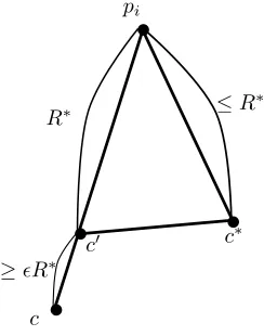
lemma first proved in [16]; when c and c∗ are the current and the optimal center respectively, we can find a point p such that d(c∗, p) = R∗ and d(c, p)2 ≥ (R∗)2 +d(c, c∗)2, which implies
d(c, c∗)2≤R2−(R∗)2. Many algorithms for the Minimum Enclosing Ball problem [6, 28] used this
lemma to improve their running time. Also in our algorithms, this lemma would guarantee a tighter bound of the distance between the current center and the optimal center, giving a better running time. However, the next lemma shows that the bound of this key lemma gets gradually relaxed as ∆ increases. When ∆ is big, d(c, c∗) can be nearly as big as R∗, which does not improve our convergence analyses.
Lemma 3.6. Letcbe the current center,c∗∈C∗ be the closest optimal center toc, andR=R(c,L)
be the radius of the minimum intersecting ball centered atc. There is an instance where(d(c, c∗))2≥
(R2−(R∗)2)2∆1 (R∗)(2− 2 2∆).
Proof. Our counterexample has n = d = ∆ + 2, and consists of n flats of different dimensions. Note that this can be easily extended to the case where all flats have the same dimension ∆, by adding at most ∆ coordinates and giving either the same fixed value or a free variable to each added coordinate.
L={l1, l2, p1, ..., p∆}. l1 andl2are of dimension ∆ and eachpi is of dimension less than ∆. Let
l1 = (−I,0,∼, ...,∼), l2 = (+I,0,∼, ...,∼) and pi = (0, ...,0, I,0,∼, ...,∼) where I > 0 appears in
thei+ 1th coordinate. In other words,pi has the firsticoordinates 0,i+ 1th coordinateI,i+ 2th
coordinate 0, and the remaining coordinates∼.
Claim 3.7. The origin is the center of unique the minimum intersecting ball, i.e. C∗={O}. Proof. Since the first coordinate ofl1andl2differ by 2I,R∗≥I. It is obvious thatBO,I intersects
all flats, since each flat has only one nonzero and nonfree coordinate of which the value is I. We argue that there is no other centercthat achievesI.
By l1 andl2, it is obvious that to achieve the radiusI, the first coordinate ofc must be zero.
We considerp1, ..., p∆ in this order. Inductively, when we look atpi and the firsticoordinates are
fixed to 0, it means that the distance fromc to each ofl1, l2, p1, ..., pi−1 in the firsticoordinates is
I. Since the value of (i+ 1)th coordinate of each of these flats is 0 or ∼, cmust have the the i+ 1 coordinate 0. Again, the distance fromcto pi in the firsti+ 1 coordinates isI, so the induction is
Letc0= (0, x2∆
, x2∆−1, ..., x2, x)I.
(d(c0, l1))2 = (1 +x2
∆+1
)I2 (d(c0, p1))2 = ((1−x2
∆
)2+x2∆)I2= (1 +x2∆+1−x2∆)I2 (d(c0, p2))2 = (x2
∆+1
+ (1−x2∆−1)2+x2∆−1)I2= (1 +x2∆+1+x2∆−x2∆−1)I2 ...
(d(c0, pi))2 = (x2
∆+1
+...+x2∆−i+3+ (1−x2∆−i+1)2+x2∆−i+1)I2= (1 +x2∆+1+...+x2∆−i+2−x2∆−i+1)I2
1 +x2∆+1+...+x2∆−i+2−x2∆−i+1 ≤1 for smallx, so (R(c0))2 = (d(c0, l1))2 = (1 +x2
∆+1
)I2. (R(c0))2−(R∗)2=x2∆+1
I2, but
(d(c∗, c0))2 ≥ x2I2
≥ (x2∆+1)2∆1 I 2 2∆I2−
2 2∆
Chapter 4
Clustering Hardness
Ak-clusteringC= (L1, ...,Ln, c1, ..., ck) is a partition ofLinto disjoint subsets (clusters) L1, ...,Lk
with centersc1, ..., ck. LetR(C) = maxiR(ci,Li) be the maximum radius of any cluster ofC, which
we also call the radius of the clustering C. Let R∗(k,L) be the optimal radius of anyk-clustering. Again, we do not useLorC in these notations when it is clear from the context.
While we have a FPTAS for the 1-center problem, that is not the case when we have a real clustering problem with k ≥2. The fundamental concept of clustering - partitioning objects into k groups so that the objects in each group are similar - has been considered in even the earliest problems in computational theory when each object corresponds to a vertex in a graph and there is an edge when two objects are similar or related; the VERTEX COVER and DOMINATING SET problem ask to findkcentersthat cover their relationships (incident edges) or directly similar objects (neighbors), respectively. k-COLORING, which is finding a partition of the vertex set intokdisjoint sets such that the subgraph induced by each set is a coclique (here, the existence of an edge means that the two vertices are different), looks more like a version of the clustering problem. Even more boldly, some variants of the 3-SAT problem can be said to look for a partition of a set of variables into 2 disjoint sets (those assigned true or false) to satisfy the given constraints, if flipping true and false does not change the satisfiability (i.e., clusters are symmetric).
Theorem 4.1. For fixed k ≥ 3 and any I, there is no algorithm that computes a I-approximate
k-clustering and runs in time polynomial of n, d,∆ unless P=N P.
Proof. We reduce the GRAPH k-COLORING problem(k ≥3) to our problem. Given G= (V, E) withV =
v1, ..., v|V| andE=
(v1,1, v1,2), ...,(v|E|,1, v|E|,2) , we construct the set ofn=|V|flats
L={l1, ..., ln} in d=|E|-dimensional coordinates. Each flat li corresponds to each vertexvi and
eachjth coordinate corresponds to each edge (vj,1, vj,2). For each 1≤i≤nand 1≤j≤m, (li)j is
decided as the following:
• vi∈/ (vj,1, vj,2): (li)j=∼, i.e. si does not have a fixed value in thejth coordinate. • vi=vj,1: (li)j=−1
• vi=vj,2: (li)j= +1
Gis k-colorable if and only if there is a k-clustering where each cluster does not have two flats that have the fixed values−1 and +1 in the same coordinate, which ensuresR∗(k,L) = 0. Therefore, G is k-colorable if and only if there is a k-clustering with R∗(k,L) = 0. If there is an algorithm that computes aI-approximatek-clustering and runs in time polynomial ofn, d,∆, we can solve the GRAPHk-COLORING problem, implyingP =N P.
Note that all the flats used in the above theorem are axis-parallel, so both axis-parallel and general case are hard whenk≥3. Since 2-COLORING is in P, a harder version of coloring(HYPERGRAPH 2-COLORING) is used to show that 2-clustering in the general (not necessarily axis-parallel) case is still hard.
Theorem 4.2. There is no algorithm that computes aI-approximate2-clustering and runs in time polynomial of n, d,∆ for anyI unless P =N P.
Proof. We reduce the SET SPLITTING problem, also known as the HYPERGRAPH 2-COLORING problem, to our problem. The SET SPLITTING problem, given a collectionSof subsets of a finite set U, decides whether there is a partition ofU into two subsetsU1 andU2 such that no subset in
S is entirely contained in eitherU1orU2. This problem remains NP-complete even if alls∈S have
|s| ≤3. Therefore, we assume that|s|= 3 for alls∈S without losing NP-completeness.
Let U = {u1, ..., un} be the given finite set, and S ={s1, ..., sm} be the collection of subsets.
For each j, sj = {uj,1, uj,2, uj,3} ⊆ S. Given such an instance, we construct the set of n flats
L = {l1, ..., ln} in d = 2m-dimensional coordinates. Think (2j−1)th and (2j)th coordinates are
associated with sj. For each 1 ≤ i ≤ n and 1 ≤ j ≤ m, (li)2j−1 and (li)2j are decided as the
following. LetA= (0,1), B= (−
√
3 2 ,−
1
2), C = (
√
3 2 ,−
1
2) be the vertices of the triangle that contains
• ui∈/sj: (li)2j−1= (li)2j=∼, i.e. si does not have a fixed value in these coordinates. • ui=uj,1: {(li)2j−1,(li)2j} ⊆R2is the line passing AandB.
• ui=uj,2: {(li)2j−1,(li)2j} ⊆R2is the line passing AandC.
• ui=uj,3: {(li)2j−1,(li)2j} ⊆R2is the line passing B andC.
... (2i−1,2i) ... (2j−1,2j) ...
l1 ... / ... ∼ ...
l2 ... \ ... / ...
l3 ... ... \ ...
[image:23.612.223.427.185.249.2]l4 ... ∼ ... ...
Table 4.1: An example whereSi ={u1, u2, u3} andSj ={u2, u3, u4}. Three lines in the same two
columns form a regular triangle around the origin.
Let (C1, C2) be a 2-clustering ofL. Iflj,1, lj,2, lj,3are in the same cluster for anyj, the minimum
intersecting ball for that cluster must cover the triangle formed in (2j−1)th and (2j)th coordinates, forcing R∗(k,L)≥1/2. Iflj,1, lj,2, lj,3 are split for every j, each cluster has at most 2 of them and
we can place the center on the intersection of those two lines, so R∗ = 0. Therefore, R∗(k,L) = 0 if and only if the given instance of the SET SPLITTING problem has a satisfactory partitioning. If there is an algorithm that computes aI-approximate 2-clustering and runs in time polynomial of n, d,∆, we can solve the SET SPLITTING problem with|s|= 3 for alls∈S, implyingP=N P.
This construction is not axis-parallel. By replacing three edges of a triangle with three vertices with some additional changes similar to the NP-hardness of 2-means[8], we can make each flat used in the reduction axis-parallel. However, in this case the inapproximability ratio reduces from infinity to a constant less than 2. In Section 6, we show a O(∆1/4)-approximation algorithm for
k= 2, indicating the fundamental difference between the axis-parallel case and the general case in 2-clustering.
Theorem 4.3. When all flats are restricted to be axis-parallel, there is no algorithm that computes a √2
3-approximate2-clustering and runs in time polynomial of n, d,∆unless P =N P.
Proof. We reduce the NOT ALL EQUAL 3-SAT problem, which is quite similar to the SET SPLIT-TING PROBLEM introduced above, to our problem. Given a set of variablesx1, ..., xn and a set
of clauses C ={C1, ..., Cm} where each Cj consists of three literals xj,1, xj,2, xj,3, negated or
un-negated, the problem asks to find the truth assignment to eachxisuch that no clause has three true
Given an instance of the NOT ALL EQUAL 3-SAT problem, we construct the set of 6m flats
L=
li,j, l0i,j|xi∈Cj ind= (n+ 2m)-dimensional coordinates. The number of flats is 6msince we
generate two flats,li,j for the literal andli,j0 for its negation, per each appearance of a literal. The
purpose of the firstncoordinates is to make sure that allli,j’s for fixediare in the same cluster and
all l0i,j’s in the other, and the purpose of remaining 2m coordinates is to penalize the clause with the three literals with the same value. For the firstncoordinates, (li,j)i= 0, (l0i,j)i=M for a large
M, and (li,j)i0 = (l0i,j)i0 =∼wheni6=i0. Therefore,li,j andl0i,j0 cannot be in the same cluster even
ifj6=j0. Since we have only two clusters, for fixedi, allli,j’s have to gather in the one cluster and
alll0
i,j’s have to gather in the other.
The (n+ 2j−1)th and (n+ 2j)th coordinates are associated withCj. For each 1≤i≤nand
1≤j, j0 ≤msuch thatxi ∈Cj (i.e. li,j ∈ L), (li,j)2j0−1, (li,j)2j0, (l0i,j)2j0−1and (li,j0 )2j0 are decided
as the following:
• j 6=j0: (li,j)2j−1= (li,j)2j= (li,j0 )2j = (l0i,j)2j=∼, i.e. li,j andl0i,j does not have a fixed value
in these coordinates.
• xi=xj,1: (li,j)2j−1= 0,(li,j)2j= 1. (l0i,j)2j−1=−
√
3 2 ,(l
0
i,j)2j =−12. Swap the role ofli,j and
l0i,j ifxj,1is negated.
• xi=xj,2: (li,j)2j−1=−
√
3
2 ,(li,j)2j =− 1 2. (l
0
i,j)2j−1=
√
3 2 ,(l
0
i,j)2j =−12. Swap the role ofli,j
andl0
i,j ifxj,2is negated.
• xi =xj,3: (li,j)2j−1=
√
3
2 ,(li,j)2j =− 1 2. (l
0
i,j)2j−1 = 0,(l0i,j)2j = 1. Swap the role ofli,j and
l0i,j ifxj,3is negated.
1 2 3 ... (2j−1,2j) ... l1,j 0 ∼ ∼ ... ↑ ...
l10,j M ∼ ∼ ... → ... l2,j ∼ 0 ∼ ... ← ...
l20,j ∼ M ∼ ... → ... l3,j ∼ ∼ 0 ... ← ...
l0
[image:24.612.227.421.480.578.2]3,j ∼ ∼ M ... ↑ ...
Table 4.2: An example whereCj= (x1,¬x2, x3). (0,1),(−
√
3 2 ,−
1 2),(
√
3 2 ,−
1
2) are represented as up,
left, right arrow vectors, respectively.
The above table shows the example of a clauseCj which consists ofxj,1=x1,¬xj,2=¬x2, xj,3=
x3. Sinceli,j andli,j0 must be separated, there are at most 23= 8 clusterings (if we do consider the
order of the clusters), and we cannot have the three same points in one cluster. Furthermore, there are exactly two cases where we can have three different points in one cluster, namelyl1,j, l02,j, l3,j in
it becomes one case). They are exactly the two assignments that make all the literals true or false at the same time. By symmetry, this argument holds for any clause with arbitrary negated or unnegated literals.
When all li,j’s gather in the one cluster and all l0i,j’s gather in the other for fixedi, the first n
coordinates do not affect the radius of the clustering at all. For each two coordinates corresponding to Cj, there are only 6 flats with fixed values, 3 for each cluster. And these flats do not have
fixed values for any other coordinate corresponding toCj0 6=Cj. Therefore, the (n+ 2j−1)th and
(n+ 2j)th coordinates of the center are decided by these coordinates of the 3 flats (either three points or two points) only, and the distances of these flats to the center are also decided by only those two coordinates. It implies that the radius of a clustering is 1 if and only if there is a clause for which each cluster corresponds to the assignment resulting in three literals with the same value. Otherwise, the radius of clustering is
√
3 2 .
Therefore, there exists a satisfying assignment to an instance of the NOT ALL EQUAL 3-SAT problem if and only if the optimal radius is
√
3
2 . If there is an algorithm that computes a 2
√
3-approximate 2-clustering and runs in time polynomial of n, d,∆, we can solve the NOT ALL
EQUAL 3-SAT problem, implyingP =N P.
The three theorems above show that it is impossible to find a good approximation algorithm that runs in time polynomial inn, d,∆, even for fixedk. We also study the case where ∆ is fixed. Similarly to what we have proved, it is impossible to find any approximation algorithm that runs in time polynomial inn, d, k, even for fixed ∆. The reduction is from the VERTEX-COVER problem.
Theorem 4.4. For fixed ∆≥1, there is no algorithm that computes a I-approximate k-clustering and runs in time polynomial ofn, d, k for anyI unlessP =N P.
Proof. We reduce the famous VERTEX COVER problem to our problem with ∆ = 1. Given G= (V, E) withV =v1, ..., v|V| andE=
(v1,1, v1,2), ...,(v|E|,1, v|E|,2) , we construct the regular
d= (|V| −1)-simplex whose|V|vertices corresponds to each vertex inV. Lconsists ofn=|E|lines where each line corresponds to each edge;li is the line passingvi,1 andvi,2.
If there is a vertex cover of size k, using the vertices in the vertex cover as centers ensures R∗(k,L) = 0, since each line contains at least one center. Conversely, if there is a k-clustering with R∗(k,L) = 0, we can move each center to some vertex while maintaining R∗ = 0 since there is no intersection of any two lines except the vertices of the simplex. Therefore, there is a vertex cover of sizek if and only if there is ak-clustering withR∗(k,L) = 0.
Again, the flats used in the reduction are not axis-parallel. By allowing a slightly larger dimension and more involved analysis, we can use the same idea to extend the proof to the axis-parallel case.
Theorem 4.5. When all flats are restricted to be axis-parallel, for fixed∆≥3, there is no algorithm that computes aI-approximatek-clustering and runs in time polynomial of n, d, kfor any I unless
P =N P.
Proof. We reduce the 3-REGULAR VERTEX COVER problem to our problem. First, we prove that the problem remains NP-hard even though all graphs are restricted to have no cycle of length
≤4. For any given graphG= (V, E), construct the graphG0 with|V|+ 2|E|vertices and 3|E|edges by splitting each edge ofGinto three edges and adding two vertices of degree two in each junction. IfGhas a vertex cover of sizek,G0has a vertex cover of sizek+|E|since if an edge ofGis covered, at least one edge ofG0 corresponding to the original edge is covered, so we need only one vertex to cover the remaining two edges ofG0 corresponding to the original edge.
For the other direction, supposeG0has a vertex cover of sizek+|E|and this vertex cover contains k0 vertices ofG. Since this vertex cover has to cover each middle edge (the middle of three pieces of the original edge) that does not contain any vertex of G(there are|E| of them), k0 ≤k. Also, if the two endpoints of any middle edge are in the vertex cover, moving one of them to the nearest vertex of Gstill ensures that all edges of G0 are covered (it is okay even if the nearest vertex was already in the cover). This may increasek0, but stillk0≤k. Now we claim that thesek0 vertices of Gform a vertex cover of G. If there is an uncovered edge of Gby these vertices, the only way to cover the three edges ofG0 is to include two new vertices into the vertex cover ofG0, but we already removed these cases. Therefore,Ghas a vertex cover of size k if and only ifG0 has a vertex cover of sizek+|E|, completing the first reduction.
Given G= (V, E) withV =
v1, ..., v|V| andE=e1, ..., e|E| , we construct the set ofn=|E|
flatsL={l1, ..., ln}ind=|V|-dimensional coordinates. Thinkjth coordinate is associated withvj.
For each 1≤i≤nand 1≤j≤m, (li)j is decided as the following: • vj is an endpoint ofei: (li)j= 1.
• vj is a neighbor of an endpoint ofei: (li)j=∼. • Otherwise: (li)j= 0.
Note that in a graph of which the maximum degree is ≤3, one edge can have at most 4 vertices (excluding its endpoints) that are adjacent to its vertices. However, using the reduction above to split each edge into three, we are sure that no adjacent vertices are both of degree 3, so each edge can have at most 3 such vertices.
For fixed j, ifc∈Rd is such thatcj= 1 andcj0 = 0 forj0 6=j,cintersects all flats corresponding
C withR(C) = 0. If there is no vertex cover of size k, for any partition of the flats(edges) into k clusters, there must be a cluster whose edges are not covered by a single vertex. There are two cases.
• There exists ei= (vx, vy), ei0 = (vz, vw) such thatx, y, z, ware different:
Note that (li)x = (li)y = 1. However, it is impossible that (li0)x =∼,(li0)y =∼, because this
implies both vx and vy are adjacent to at least one of vz and vw, which results in a cycle of
length 3 or 4. There must be at least one coordinate in whichliis 1 andli0 is 0, implying that
R∗(k,L)>0.
• Each pair of edges shares an endpoint:
Take any edge (vx, vz) from this cluster. Since this cluster is not covered by either vx or vz,
there must be an edgeei= (vx, vy) andei0 = (vz, vw) for somey6=zandw6=x. y=wmeans
a cycle of length 3, soy6=w, implying that x, y, z, ware all different again.
Therefore,Gadmits a vertex cover of sizekif and only ifR∗(k,L) = 0. If there is an algorithm that computes aI-approximatek-clustering and runs in time polynomial ofn, d, kfor anyI, we can solve the 3-REGULAR VERTEX COVER problem, implyingP =N P.
Note that our reductions do not increase the size of each instance much. Therefore, if we assume the exponential time hypothesis formalized in [20], which implies that the 3-SAT problem cannot be solved in 2o(n), our reductions also imply that we cannot expect an algorithm whose running time
is subexponential ink or ∆, with the only exception being the axis-parallel case for fixed ∆.
Theorem 4.6. Assuming the exponential time hypothesis, for fixedk≥3, there is no algorithm that computesI-approximatek-clustering and runs in time 2o(∆)poly(n, d), both for the general and the
axis-parallel case for anyI. For fixed ∆≥1, there is no such algorithm for the general case which runs in time 2o(k)poly(n, d). In the axis-parallel case, for fixed ∆ ≥3, there is no such algorithm
which runs in time 2o(√k)poly(n, d).
Proof. Note that if there is an approximation algorithm with any factorI, the problems that have been used in our reductions will be solved because all of our reductions mapped the accepting instances to the clustering instances withR∗= 0, and the rejecting instances to those withR∗>0.
Assuming the exponential time hypothesis, the 3-SAT problem, the GRAPH 3-COLORING problem, and the VERTEX COVER problem (withk as a part of input, not a parameter) cannot be solved in time 2o(n+m), where n is the number of vertices (variables) andm is the number of
For fixed ∆, our reduction in Theorem 4.4 preserveskin the original VERTEX-COVER problem, so we cannot have a subexponential (ink) algorithm in the general case. In the axis-parallel case, the reduction from the 3-SAT problem to the 3-REGULAR VERTEX COVER problem increases the size (n+m) of the problem at most quadratically [15], and the reduction to the 3-REGULAR VERTEX COVER without any cycle of length≤4 in Theorem 4.5 increases the size of the graph linearly(n0 = n+ 2m, m0 = 3m). Therefore, an algorithm for the axis-parallel case which runs in time 2o(
√
k)poly(n, d) solves the 3-REGULAR VERTEX COVER problem in time 2o(√n+m)and the
Chapter 5
Clustering Algorithms
In the previous section, we showed that there cannot be any polynomial time approximation algo-rithm even when one ofkor ∆ is fixed. Therefore, the natural next step is to find an approximation algorithm which is fast for smallk and ∆. Using Algorithm 2 (Moving Center) for computing the minimum intersecting ball, we can obtain a PTAS whose running time is linear innanddfor fixedk and ∆. Note that algorithm 2 starts with an initial center whose distance to the closest optimal cen-ter is bounded byO(√∆R∗). However, in clustering, it is impossible, becauseR∗ can be arbitrarily small compared to maxj(Mj−mj); given two points, the radius of the minimum enclosing ball is
at least half of the distance between these points, but the radius of the optimal clustering becomes zero when we allow two clusters. Thus, we need to study how Algorithm 2 behaves if it starts with an arbitrary center. Fortunately, with some modification on the algorithm, this does not affect the running time greatly. Since the difference between the optimal center and the current center in the jth coordinate is bounded byR∗once thejth coordinate isconsidered (the center has move to a flat with a fixed value for the jth coordinate), and we have only ∆ unconsidered coordinates after the first move, we need only ∆ + 1 additional steps to move to a reasonable position. Figure 5.1 shows a simple example in which an arbitrary initial center moves to the desired position in 2 = ∆ + 1 steps.
Theorem 5.1. If all flats are axis-parallel andR∗ is given, Algorithm 2 with an arbitrary initial centerc computes an intersecting ball with radiusR < R∗(1 +)in timeO(nd∆(12 + 1)).
start
end
Proof. Letai⊆[d] be the set of the indices of the coordinates in whichlihas fixed values. |ai|=d−∆
for eachi. Since we assumed that there is no coordinate in which every flat does not have a fixed value, the union ofaiover all 1≤i≤nis [d]. Letc∗∈C∗be an arbitrary optimal center. Without
loss of generality, letli be the flat chosen in theith iteration,ci be the current center after the ith
iteration, and bi =∪ij=1ai. In other words,bi is the set of coordinates in which the current center
has moved at least once. Letdai(p, q) =dl⊥
i(p, q) = qP
j∈ai(pj−qj)
2. d
bi is also defined similarly. We classify eachith iteration into one of two categories depending on whetherai⊆bi−1 or not. If
ith iteration belongs to the former, the analysis of Algorithm 2, applied to the case where we only consider the coordinates inbi−1 =bi, shows that (dbi(ci, c
∗))2 is decreased by at least Ω(R∗ 2) from
(dbi−1(ci−1, c
∗))2. Otherwise, the same analysis cannot be applied sinceb
i−16=bi, but the fact that
(dai(ci, c
∗))≤2R∗ shows that
(dbi(ci, c
∗))2 = X
j∈ai
((ci)j−(c∗)j)2+
X
j∈bi−1−ai
((ci)j−(c∗)j)2
≤ X
j∈ai
((ci)j−(c∗)j)2+
X
j∈bi−1−ai
((ci−1)j−(c∗)j)2 ≤ 4(R∗)2+ (dbi−1(ci−1, c
∗))2
Therefore, (dbi(ci, c
∗))2 is increased by at mostO((R∗)2) from (d
bi−1(ci−1, c
∗))2. The first iteration
makes |b1| = |a1| = d−∆, so there are at most ∆ + 1 iterations of the second category and
(dbi(ci, c
∗))2 is increased at most by O(∆(R∗)2) totally during the algorithm. Since each iteration
of the first category decreases (dbi(ci, c
∗))2by Ω(R∗
2), and there are at mostO(
∆
2) iterations of the
first category. Therefore the total number of iterations isO(∆(1
2 + 1)).
Combined with the technique used in [6], where we pick a far point from the current centers and
guess the cluster to which it belongs, the above theorem enables us to find a (1 +)-approximate clustering when we know the optimal radiusR∗(k,L).
Theorem 5.2. If all flats are axis-parallel andR∗ is given, a (1 +)-approximatek-clustering can be found in time2O(∆klogk(1+12))nd.
Proof. LetC∗= (L∗
1, ...,L∗k, c∗1, ..., c∗k) be an optimal clustering. We start from the centersc1, ..., ck
at arbitrary positions.
The algorithm picks li that maximizes the minimum distance to each c1, ..., ck. If d(li, cj) ≤
(1+)R∗for everyjthen∪j∈[k]B(cj,(1+)R∗) intersects every flat inLand we are done. Otherwise,
exhaustively guess thejth cluster such thatd(cj, li)>(1 +)R∗and movecj tolias in Algorithm 2.
If we guess correctly, d(li, cj)≤ (1 +)R∗ for each li ∈ L∗j in O(∆(1 +12)) iterations where jth
guessing between at most k clusters and can be implemented in time O(nd). Therefore, the total running time is 2O(∆klogk(1+12))nd.
As in the 1-center problem, guessing the optimal radius R∗ can be done by using binary search. Finding a meaningful upper bound onR∗ uses the main algorithm with the radius 0.
Theorem 5.3. If all flats are axis-parallel, running the above clustering algorithm with the guessed optimal radius zero will find the clustering with the radius at mostO(√∆R∗)in time2O(∆klogk)nd.
Proof. As above, letli be the flat chosen in theith iteration,ai⊆[d] be the set of the indices of the
coordinates in which li has the fixed value. We also define ci,j to be the center of the jth cluster
after theith iteration, and bi,j to be the union of ak’s (1≤k≤i) that belong to the jth cluster.
For any pair of (i, j) such that bi,j 6= ∅ (i.e. at least one flat is classified to the jth cluster), let
lk(k ≤i) be the last flat to which the center of the jth cluster has moved. As the above proofs,
dak(ci,j, c
∗
j)≤R∗ and for each coordinate qin bi−ak (at most ∆ of them), |(ci,j)q−(c∗j)q| ≤R∗.
Therefore, (dbi,j(ci,j, c
∗
j))2≤∆(R∗)2.
In theith iteration, letj be the cluster thatlibelongs to in the optimal clustering. Ifai⊆bi−1,j,
d(li, ci−1,j) = dbi−1,j(li, ci−1,j) ≤ dbi−1,j(li, c
∗
j) +dbi−1,j(c
∗
j, ci−1,j)≤ O( √
∆R∗). Since li is chosen
as the flat that maximizes the minimum distance to any current center, d(li, ci−1,j) ≤O( √
∆R∗) means that the distance from any flat to its nearest center is O(√∆R∗). Otherwise, the size of
bi,j =bi−1,j∪ai grows strictly. Since the first classification makes|bi,j|=d−∆, there are only ∆ + 1
iterations for one cluster to grow bi,j strictly. Therefore, in O(k∆) iterations, we are guaranteed
to have a situation where the radius of the current clustering isO(√∆R∗). Each iteration involves guessing the correct cluster thatli belongs to, so the total running time is 2O(∆klogk)nd.
Therefore, we need O(∆) trials of binary search to guess the optimal radius with error < . Guessing the optimal radius and trying for different values of the optimal radius does not increase the asymptotic complexity of the main algorithm, so the total running time is 2O(∆klogk(1+12))nd.
Chapter 6
2-Clustering of axis-parallel flats
Section 4 shows that for fixed k ≥2 it is impossible to have any approximation algorithm in the general case. When all flats are restricted to be axis-parallel, this threshold is increased by 1. If k= 2, the lower bound of the approximation ratio for the axis-parallel case shown in Theorem 4.3 is
2
√
3, which is quite different from the other cases. This leads to the natural conjecture that there is
a polynomial time(inn, d,∆) approximation algorithm for the axis-parallel 2-center problem. One reason that makes this conjecture more plausible is the relationship between the problems we reduced to prove the hardness results of our problem. The hardness of 2-clustering in the general case is shown by the reduction from the HYPERGRAPH 2-COLORING problem, and the hardness of 3-clustering in the axis-parallel case is shown by the reduction from the GRAPH 3-COLORING problem. In these reductions, there is a natural correspondence between the number of colors/the number of centers, hypergraphs/non-axis parallel flats, and regular graphs/axis-parallel flats. Therefore, that GRAPH 2-COLORING is in P motivates us to find an approximation algorithm for this special axis-parallel 2-clustering problem, whose existence will show the fundamental difference between the axis-parallel case and the general case in terms of approximability.
In fact, we can find a polynomial time approximation algorithm for the axis-parallel 2-clustering problem by solving a problem similar to GRAPH-2-COLORING as a subroutine. To do this, we need another Helly-type theorem which holds specifically for axis-parallel flats. It extends the relatively trivial fact that pairwise nonempty intersection of some set of axis-parallel flats implies all of them intersect. Similarly, if any pairwise distance of some set of flats is small, there is a small intersecting ball.
Theorem 6.1. Let L ={l1, ..., ln} be the set of axis-parallel flats, where each li is of dimension
∆i < d. If d(li, lj)≤r for every 1≤i, j ≤n,R∗(L)<2d
1
4r. In other words, if any pair of slabs
li+BO,r
2 intersect, then all slabs
n
li+BO,d1 4r
o
largest fixed value for thejth coordinate, are defined for eachj. Let r0 = maxj(Mj−mj) be the
longest edge of the hypercube [m1, M1]×...×[md, Md]. It is clear thatr≥r0.
Let ∆ = mini∆i. Assume without loss of generality dim(l1) = ∆ and l1 has the fixed value
in 1, ...,(d−∆)th coordinate. If ∆≥d−p for some p, c = (m1+M1
2 , ...,
md+Md
2 ) makes d(c, li)≤
√
d−dim (li)r0
2 ≤
√
pr
2 for eachi, so R
∗(L)≤ √pr
2 .
If ∆ < d−p, fix (c)j = (l1)j for j = 1, ..., d−∆. (d[d−∆](c, li))2 ≤(d(l1, li))2 ≤ r2 for all i.
Since we have fixed the first d−∆ coordinates and d[d]−[d−∆](li, lj) ≤d(li, lj) ≤r, we can apply
the same argument recursively where the dimension of the entire space is ∆ < d−p. Therefore, (R∗(L))2≤r2+ (R∗(L0))2whereL0={l0
2, ..., l0n}andli0 ∈R∆is the projection oflitol1(1< i≤n).
Let p=l√dm and prove the theorem by the induction on the underlying dimensiond. When d = 1 it holds trivially. When the theorem is true for every 1, ..., d−1, R∗(L) ≤
√
pr
2 ≤ 2d
1 4r
or (R∗(L))2 ≤ r2 + (R∗(L0))2 where L0 is the set of flats in the Euclidean space of dimension
d−p≤d−√dwith the smaller pairwise distance. By the induction hypothesis,
(R∗(L))2 ≤ r2+ 4r2 q
d−√d = (1 + 4
q
d−√d)r2
≤ 4r2√d
since (1 + 4pd−√d)2 = (1 + 8pd−√d+ 16(d−√d)) ≤ 16d. Therefore, the induction is complete andR∗(L)<2d1
4r.
The next theorem shows that this Helly-type theorem for axis-parallel flats is tight in terms of the radius of an intersecting ball.
Theorem 6.2. There is a set of axis-parallel flatsL ={l1, ..., ln} in Rd such thatd(li, lj)≤rfor
every 1≤i, j≤n, andR∗(L) = Ω(d14)r.
Proof. Letd= (n−1)nand partition the coordinates intonblocks each of which consists of (n−1) coordinates. For 1≤i6=j≤n, define
p(i, j) =
j, ifj < i j−1, ifj > i
(li)j=
0, ifi=q
1, i6=qandj−(q−1)(n−1) =p(q, i)
∼, otherwise
In other words, (li) has all 0’s in theith block and exactly one 1 in each of the other blocks, but
the position of 1 in each block is different for each flat. Obviously, each pairwise distance isr=√2, since the only two coordinates whereli andlj are fixed and differ are the position in theith block
wherelj has 1 and the position in thejth block whereli has 1.
Let c = (c1, ..., cd) ∈ Rd be an arbitrary center. For each coordinate j, there is exactly one flat that has 1 in this coordinate and exactly one flat that has 0 in this coordinate. Therefore, P
1≤i≤n((li)j −(cj))2 ≥ 12 with equality if and only if cj = 12. Summing over all coordinates,
P
1≤i≤n(d(c, li))
2 ≥d/2 = n(n−1)
2 with equality ifc = ( 1 2, ...,
1
2). Therefore, max1≤i≤n(d(c, li)) 2 ≥
n−1 2 so R
∗(L)≥qn−1 2 =
√
n−1
2 r= Ω(d
1 4)r.
Equipped with this new Helly-type Theorem 6.1, we give a polynomial time approximation algorithm for the axis-parallel 2-clustering problem. Note thatd(li, lj)≤2R∗whenliandljbelong to
the same cluster in the optimal clustering. Therefore, we can construct a graph based on the pairwise distances, use a 2-COLORING algorithm to get two clusters; Within each cluster, Theorem 6.1, applied to the flats projected to one of them, ensures that they can be covered by a ball of radius O(∆1/4)R∗.
Theorem 6.3. If all flats are axis-parallel, anO(∆14)-approximate2-clustering can be found in time
O(dn2logn).
Proof. Note thatd(li, lj)≤2R∗whenli andlj belong to the same cluster in the optimal clustering.
Letr be the maximum d(li, lj) that is not larger than 2R∗. Construct a graph G= (L, E) where
(li, lj)∈E if and only ifd(li, lj)> r. ThenGis 2-colorable since there is one corresponding to the
optimal clustering. Find a 2-coloring; each color represents a cluster so thatd(li, lj)≤rfor anyi, j
in the same cluster.
Without loss of generality, let l1, ..., ln0 belong to the same cluster. Letl01,j belj projected into
l1. For any 1< j, k≤n0,dl1(l 0
1,j, l10,k) =dl1(lj, lk)≤d(lj, lk)≤2R
∗. By Theorem 6.1 applied to l
1
(of dimension ∆), there existsc∈l1such thatdl1(c, lj) =dl1(c, l 0
1,j)≤O(∆
1
4)R∗ for any 1≤j≤n0.
Since dl⊥
1(c, lj) =dl1⊥(l1, lj)≤2R
∗, so d(c, l
j)≤ O(∆
1
4)R∗ for any 1≤j ≤n0. This analysis also
works for the other cluster, so we found anO(∆14)-approximate 2-clustering.
Chapter 7
Conclusions and Future Work
We have presented the algorithms and hardness results for clustering affine subspaces. Our main algorithm for generalkand ∆ and hardness results almost match in the sense that we proved that the exponential dependence on k and ∆ is inevitable and suggested an algorithm which runs in time exponential in k and ∆ but linear in n and d. Furthermore, assuming the exponential time hypothesis, the exponent linear in ∆ (for fixedk) and quasi-linear ink(for fixed ∆) is almost tight because we cannot expect a subexponential(for any ofk and ∆) algorithm in the general case; the axis-parallel case only relaxes the dependence onkfrom 2o(k)to 2o(√k). Therefore, other than trying
to find a subexponential (ink) algorithm for the axis-parallel case, one immediate improvement of the running time will be to reduce the current quasi-multilinear exponent 2O(∆klogk) to a
quasi-linear one like 2O(∆+klogk). If this improvement is achieved, it will be nearly the theoretically
fastest algorithm. Conversely, there might be another reduction that, by considering generalkand ∆ simultaneously, proves it is impossible to have an algorithm which runs in time 2o(∆k); in this case, our algorithm will nearly match the lower bound. Since our algorithms are all deterministic and do not assume instances are easily clusterable, it is also tempting to try to exploit the power of randomness or to assumewell-clusterability or stabilityintroduced in[27, 4, 3, 22] on the instances to improve the running time.