Diffraction by a Terminated, Semi-Infinite Parallel-Plate Waveguide with Four-Layer Material Loading

DIFFRACTION BY A TERMINATED, SEMI-INFINITE PARALLEL-PLATE WAVEGUIDE WITH FOUR-LAYER MATERIAL LOADING

E. H. Shang and K. Kobayashi

Department of Electrical, Electronic, and Communication Engineering

Chuo University Tokyo 112-8551, Japan

Abstract—The plane wave diffraction by a terminated, semi-infinite parallel-plate waveguide with four-layer material loading is rigorously analyzed using the Wiener-Hopf technique. Introducing the Fourier transform for the unknown scattered field and applying boundary conditions in the transform domain, the problem is formulated in terms of the simultaneous Wiener-Hopf equations satisfied by the unknown spectral functions. The Wiener-Hopf equations are solved via the factorization and decomposition procedure leading to the exact solution. The scattered field in the real space is evaluated by taking the inverse Fourier transform and using the saddle point method. Representative numerical examples of the radar cross section (RCS) are presented, and the far-field scattering characteristics of the waveguide are investigated in detail.

1. INTRODUCTION

Analysis of the scattering from open-ended metallic waveguide cavities has received much attention recently in connection with the prediction and reduction of the radar cross section (RCS) of a target [1–6]. This problem serves as a simple model of duct structures such as jet engine intakes of aircrafts and cracks occurring on surfaces of general complicated bodies. Therefore, investigation of the scattering mechanism in case of the presence of open cavities is an important subject in the area of the RCS prediction and reduction. In addition, it is often desirable to reduce the backscattering from such cavities for

applications to the aircraft scattering studies. Two typical methods employed for this purpose are, (i) loading the interior of the cavity with a lossy material, and (ii) shaping the cavity. From the viewpoint of these engineering applications, a number of scientists have thus far analyzed the diffraction problems involving various two- and three-dimensional (2-D and 3-D) cavities by means of high-frequency ray techniques and numerical methods [7–13]. It appears, however, that the solutions obtained by these approaches are not uniformly valid for arbitrary cavity dimensions. There are also important contributions to studies on the cavity RCS based on a rigorous function-theoretic approach based on the Wiener-Hopf technique [14, 15].

The Wiener-Hopf technique [16–18] is one of the powerful approaches for analyzing wave scattering and diffraction problems associated with canonical geometries, which is mathematically rigorous in the sense that the edge condition, required for the uniqueness of the solution, is explicitly incorporated into the analysis. In the previous papers, we have carried out a rigorous RCS analysis of 2-D cavities of various shapes formed by a finite parallel-plate waveguide [19– 26] and by a semi-infinite parallel-plate waveguide [27, 28] using the Wiener-Hopf technique. It has been clarified that our final solutions are valid over a broad frequency range and can be used for validating commonly used numerical methods and high-frequency ray techniques. This paper serves as an important generalization to our previous analysis [27, 28] for the terminated, semi-infinite parallel-plate waveguide with three-layer material loading. We shall consider in this paper a terminated, semi-infinite parallel-plate waveguide with four-layer material loading, and analyze the E-polarized plane wave diffraction by means of the Wiener-Hopf technique. Our final solution is shown to be uniformly valid for arbitrary waveguide dimensions. The cavity structure considered in this paper can be regarded as a simple model of cracks occurring on surfaces of complicated bodies. Therefore by loading interior regions of the cracks with multi-layer materials, unnecessary backscattering waves can be reduced. The results presented in this paper may contribute to the progress in the area of research on the RCS prediction and reduction.

which are then led to efficient approximate solutions of the Wiener-Hopf equations. It is to be noted that that our final solution is uniformly valid for arbitrary waveguide dimensions. The scattered field is evaluated explicitly by taking the inverse Fourier transform together with the use of the saddle point method. The field inside the waveguide is expressed in terms of the TE modes, whereas for the field outside the waveguide, an asymptotic expression of the scattered far field is derived in two difference forms. We shall present illustrative numerical examples of the RCS for various physical parameters to discuss the backscattering characteristics in detail. In particular, it is shown that significant RCS reduction can be achieved by loading the interior of the cavity with a four-layer lossy material.

The time factor is assumed to bee−iωt, and suppressed throughout this paper.

2. FORMULATION OF THE PROBLEM

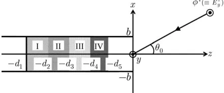
We consider the diffraction of an E-polarized plane wave by a terminated, semi-infinite parallel-plate waveguide with four-layer material loading, as shown in Fig. 1, where the waveguide plates are infinitely thin, perfectly conducting, and uniform in the y-direction. The material layers I (−d1 < z < −d2), II (−d2 < z < −d3),

III (−d3 < z < −d4), and IV (−d4 < z < −d5) are characterized by

the relative permittivity/permeability (εm, µm) form= 1, 2, 3, and 4, respectively.

Figure 1. Geometry of the problem.

Let the total electric fieldφt_{(x, z) [≡E}t

y(x, z)] be

φt(x, z) =φi(x, z) +φ(x, z), (1) whereφi(x, z) is the incident field of E polarization defined by

φi(x, z) =e−ik(xsinθ0+zcosθ0)_{, 0< θ}

with k[≡ ω(ε0µ0)1/2] being the free-space wavenumber. We shall

assume that the vacuum is slightly lossy as in k = k1 +ik2 with

0< k2 k1, and take the limitk2→+0 at the end of analysis.

The total fieldφt(x, z) satisfies the 2-D Helmholtz equation

∂2/∂x2+∂2/∂z2+µ(x, z)ε(x, z)k2φt(x, z) = 0, (3) where

µ(x, z) =           

µ1(layer I)

µ2(layer II)

µ3(layer III)

µ4(layer IV)

1(otherwise)

, ε(x, z) =           

ε1(layer I)

ε2(layer II)

ε3(layer III)

ε4(layer IV)

1(otherwise)

. (4)

Nonzero components of the total electromagnetic fields are derived from

E_yt, H_xt, H_zt =

φt, i ωµ0µ(x, z)

∂φt ∂z ,

1 iωµ0µ(x, z)

∂φt ∂x

. (5)

It follows from the radiation condition that

φ(x, z) =

Oek2zcosθ0 _asz→ −∞_,

Oe−k2z _asz→ ∞_. (6)

We now define the Fourier transform of the scattered field as

Φ(x, α) = (2π)−1/2

_∞

−∞φ(x, z)e

iαz_{dz, α= Reα+iImα(≡σ+iτ).} (7)

In the view of the radiation condition, it is found that Φ(x, α) is regular in the strip −k2 < τ < k2cosθ0 of the complexα-plane. Introducing

the Fourier integrals as

Φ+(x, α) = (2π)−1/2

_∞

0

φ(x, z)eiαzdz, (8)

Φ₋(x, α) = (2π)−1/2 0

−∞φ

t_{(x, z)e}iαz_{dz, (9)}

Φ(₁m)(x, α) = (2π)−1/2

₋dm+1

−dm

φt(x, z)eiαzdz, form= 1,2,3,4,(10)

Φ(5)₁ (x, α) = (2π)−1/2 0

−d5

it is found that Φ+(x, α) and Φ−(x, α) are regular in τ > −k2 and

τ < k2cosθ0, respectively, whereas Φ(1m)(x, α) for m= 1, 2, 3, 4, and

5are entire functions. In the following, we shall use the subscript ‘1’ for entire functions as well as the subscripts ‘+’ and ‘−’ for functions regular in τ >−k2 and τ < k2cosθ0, respectively. Using (7)–(11), we

can express Φ(x, α) as

Φ(x, α) =

Ψ₍₊₎(x, α) + Φ₋(x, α) for |x|> b, Ψ₍₊₎(x, α) + Φ1(x, α) for |x|< b,

(12)

where

Φ1(x, α) = 5

m=1

Φ(₁m)(x, α), (13)

Ψ₍₊₎(x, α) = Φ+(x, α)−

e−ikxsinθ0

(2π)1/2_{i(α−kcosθ} 0)

. (14)

It is seen from (14) that Ψ(+)(x, α) is regular inτ >−k2 except for a

simple pole atα=kcosθ0. The subscript ‘(+)’ will be used hereafter

for functions with this property.

In order to derive transformed wave equations, we note that

∂2/∂x2+∂2/∂z2+k2 φ(x, z) = 0 (15)

holds except for the material-loaded regions, and that

∂2/∂x2+∂2/∂z2+k2_m φt(x, z) = 0 (16) form= 1, 2, 3, and 4 hold for the regions I, II, III, and IV, respectively, wherekm = (µmεm)1/2k. For the region|x|> b, we can show by taking the Fourier transform of (15) and using (6) that

d2/dx2−γ2 Φ(x, α) = 0 (17)

holds in the strip−k2< τ < k2cosθ0,where

γ = (α2−k2)1/2, Reγ >0. (18) Equation (17) is the transformed wave equation for|x|> b.

The derivation of transformed wave equations for the region

boundary condition for tangential electromagnetic fields at z =−d5,

we derive that

d2/dx2−γ2 Φ(5)₁ (x, α)+Ψ(+)(x, α)

=e−iαd5_[(1/µ

4)f4(x)−iαg4(x)]

(19)

forτ >−k2 withα=kcosθ0, where

f4(x) = (2π)1/2

∂φt(x,−d4−0)

∂z , (20)

g4(x) = (2π)1/2φt(x,−d4). (21)

Next we multiply both sides of (16) by (2π)−1/2_eiαz _{and integrate} with respect to z over the ranges −d1 < z < −d2, −d2 < z < −d3,

−d3 < z < −d4,and −d4 < z <−d5. Using the boundary conditions

for tangential electromagnetic fields at z = −dm for m =1, 2, 3, 4, and 5, we obtain that

d2/dx2−Γ2₁ Φ(1)₁ (x, α) = e−iαd1_f

+(x)−e−iαd2[f1(x)−iαg1(x)],(22)

d2/dx2−Γ2₂ Φ(2)₁ (x, α) = e−iαd2_[(µ

2/µ1)f1(x)−iαg1(x)]

−e−iαd3_[f

2(x)−iαg2(x)], (23)

d2/dx2−Γ2₃ Φ(3)₁ (x, α) = e−iαd3_[(µ

3/µ2)f2(x)−iαg2(x)]

−e−iαd4_[f

3(x)−iαg3(x)], (24)

d2/dx2−Γ4 Φ(4)1 (x, α) = e−

iαd4_[(µ

4/µ3)f3(x)−iαg3(x)]

−e−iαd5_[f

4(x)−iαg4(x)] (25)

for all α, where Γm = (α2−k_m2)1/2 with ReΓm >0 for m= 1,2,3,4, and

f+(x) = (2π)−1/2

∂φt(x,−d1+ 0)

∂z , (26)

fm(x) = (2π)−1/2 ∂φ

t_(x,−dm

+1−0)

∂z m= 1,2,3, (27)

gm(x) = (2π)−1/2φt(x,−dm+1) m= 1,2,3. (28)

Equations (19) and (22)–(25) are the desired transformed equations for|x|< b.

In view of (6) and (7), it follows that Φ(x, α) is bounded for

|x| → ∞, and hence, the solution of (17) is expressed as

Φ(x, α) =

Ψ(+)(b, α)e−γ(x−b) forx > b,

Ψ(+)(−b, α)eγ(x+b) for x <−b,

where we have used (12) and the following boundary conditions for tangential electric fields acrossx=±b:

Φ₋(±b±0, α) = 0, Φ1(±b∓0, α) = 0, (30)

Φ+(±b+ 0, α) = Φ+(±b−0, α)[≡Φ+(±b, α)]. (31)

Equation (29) gives the scattered field representation for|x|> b. For region |x| < b, the transformed wave equations involve the unknown inhomogeneous terms f+(x) and fm(x), gm(x) for m = 1,2,3,4 due to the medium discontinuities (see (19) and (22)–(25)). In view of the edge condition [17], it follows that f+(x), fm(x), and gm(x) behave like O[(x∓b)−1+ν] as x → ±b, where ν is a constant satisfying 0 < ν < 1 which depends on the relative permeability µm for m = 1,2,3,4. Therefore we can expand these functions into the convergent Fourier sine series as in

f+(x) =

1 b

∞

n=1

f_n+sinnπ

2b (x+b), (32)

fm(x) gm(x)

= 1

b

∞

n=1

fmn gmn

sinnπ

2b(x+b) (33)

for|x|< b. Solving the transformed wave equations with the aid of (30) and (31) and carrying out some manipulations, we derive the solutions of (19) and (22)–(25) with the result that

Φ(5)₁ (x, α) + Ψ(+)(x, α)

= Ψ₍₊₎(b, α)sinhγ(x+b)

sinh 2γb −Ψ(+)(−b, α)

sinhγ(x−b) sinh 2γb

−1

b

∞

n=1

c5n(α)

α2_+γ2

n sinnπ

2b(x+b), (34)

Φ(₁m)(x, α) = −1 b

∞

n=1

cmn(α) α2_{+ Γ}2

mn sinnπ

2b(x+b), m= 1,2,3,4, (35)

where

γn =

(nπ/2b)2−k2 1/2

, Γmn= [(nπ/2b)2−km2]1/2, (36)

c5n(α) = e−iαd5c−5n(α), (37)

cmn(α) = e−iαdm_c+

with

c+_1n(α) = f_n+, c₂−_n(α) =f1n−iαg1n, (39)

c+_2n(α) = (µ2/µ1)f1n−iαg1n, c−3n(α) =f2n−iαg2n, (40)

c+_3n(α) = (µ3/µ2)f2n−iαg2n, c−4n(α) =f3n−iαg3n, (41) c+_4n(α) = (µ4/µ3)f3n−iαg3n, c−5n(α) =f4n−iαg4n. (42) Here the Fourier coefficients f_n+ and fmn, gmn for m = 1,2,3,4 are defined by (A5)–(A7) in Appendix A. Substituting (32) and (33) into (12), the scattered field representation for region|x|< bis derived.

Summarizing the above results, we derive that

Φ(x, α) = Ψ(+)(±b, α)e∓γ(x∓b) forx >< ±b,

= Ψ(+)(b, α)

sinhγ(x+b)

sinh 2γb −Ψ(+)(−b, α)

sinhγ(x−b) sinh 2γb −1 b ∞ n=1

c5n(α) α2_+γ2

n sinnπ

2b(x+b)

−1 b 4 m=1 ∞ n=1

cmn(α) α2_{+ Γ}2

mn sinnπ

2b(x+b) for |x|< b, (43)

Equation (43) is the scattered field representation in the Fourier transform domain and holds the strip−k2< τ < k2cosθ0.

We now differentiate (43) with respect to x and set x = ±b± 0,±b∓0 in the results. Carrying out some manipulations with the aid of boundary conditions, we obtain that

J₋d(α) =−U(+)(α) M(α) −

∞

n=1,odd

nπ b2

c5n(α) α2_+γ2

n +

4

m=1

cmn(α) α2_{+ Γ}2

mn

, (44)

J₋s(α) =−V(+)(α) N(α) +

∞

n=2,even

nπ b2

c5n(α)

α2_+γ2

n + 4 m=1 cmn(α) α2_{+ Γ}2

mn

, (45)

where

U(+)(α) = Ψ(+)(b, α) + Ψ(+)(−b, α), (46)

V₍₊₎(α) = Ψ₍₊₎(b, α)−Ψ₍₊₎(−b, α), (47)

J₋d,s(α) = J₋(b, α)∓J₋(−b, α), (48) J₋(±b, α) = Φ₋(±b±0, α)−Φ₁(±b∓0, α), (49)

M(α) = e−

γb_coshγb

γ , N(α) =

e−γbsinhγb

In (49), the prime denotes differentiation with respect to x. Equations (44) and (45) are the desired simultaneous Wiener-Hopf equations satisfied by the unknown functions. In the next section, we will solve the Wiener-Hopf equations, and derive exact and approximate solutions.

3. SOLUTION OF THE WIENER-HOPF EQUATIONS

The kernel functions M(α) and N(α) given by (50) are factorized as [16, 17]

M(α) =M+(α)M−(α), N(α) =N+(α)N−(α), (51)

where

M+(α)[=M−(−α)]

= (coskb)1/2eiπ/4(k+α)−1/2·exp{(iγb/π) ln [(α−γ)/k]}

·exp{(iαb/π) [1−C+ ln(π/2kb) +iπ/2]}

· ∞

n=1,odd

(1 +α/iγn)e2iαb/nπ, (52)

N+(α)[=N−(−α)]

= (sinkb/k)1/2exp{(iγb/k) ln[(α−γ)/k]}

·exp{(iαb/π) [1−C+ ln(2π/kb) +iπ/2]}

· ∞

n=2,even

(1 +α/iγn)e2iαb/nπ (53)

withC (= 0.57721566· · ·) being Euler’s constant. It is seem from (50) and (51) thatM_±(α) andN_±(α) are regular and nonzero inτ >_< ∓k2,

and show the asymptotic behavior

M_±(α)∼(∓2iα)−1/2, N_±(α)∼(∓2iα)−1/2 (54)

asα→ ∞ withτ >_< ∓k2.

resultant equation. This leads to

M₋(α)J₋d(α) +

2 π

1/2

icos(kbsinθ0)

M+(kcosθ0)(α−kcosθ0)

+

∞

n=1,odd

nπ b2

1 α+iγn

M₋(α)c5n(α) α−iγn

+M+(iγn)c5n(−iγn) 2iγn + 4 m=1 1 α+iΓmn

M₋(α)cmn(α) α−iΓmn

+M+(iΓmn)cmn(−iΓmn) 2iΓmn

=−U(+)(α) M+(α)

+

2 π

1/2 _icos(kbsinθ 0)

M+(kcosθ0)(α−kcosθ0)

+

∞

n=1,odd

nπ 2b

M+(iγn)c5n(−iγn)

biγn(α+iγn) +

4

m=1

M+(iΓmn)cmn(−iΓmn)

biΓmn(α+iΓmn)

.(55)

It is seen that the left-hand and right-hand sides of (53) are regular in the lower (τ < k2cosθ0) and upper (τ >−k2) half-planes, respectively,

and both sides have a common strip of regularity−k2 < τ < k2cosθ0.

Hence, the argument of analytic continuation shows that both sides of (53) must be equal to an entire function, which is found to be identically zero by taking into account the edge condition and Liouville’s theorem. Therefore, it follows that

U₍₊₎(α) M+(α) −

2 π

1/2

icos(kbsinθ0)

M+(kcosθ0)(α−kcosθ0)

−

∞

n=1,odd

nπ 2b

M+(iγn)c5n(−iγn) biγn(α+iγn) +

4

m=1

M+(iΓmn)cmn(−iΓmn) biΓmn(α+iΓmn)

= 0.

(56)

A similar procedure can be applied for decomposition of the Wiener-Hopf equation (43). Multiplying both sides of (43) byN₋(α) and decomposing the resultant equation, we arrive at

V₍₊₎(α) N+(α) −

2 π

1/2

sin(kbsinθ0)

N+(kcosθ0)(α−kcosθ0)

+

∞

n=2,even

nπ 2b

N+(iγn)c5n(−iγn) biγn(α+iγn) +

4

m=1

N+(iΓmn)cmn(−iΓmn) biΓmn(α+iΓmn)

= 0.

It should be noted that the unknown coefficients c5n(−iγn) and cmn(−iΓmn) are involved in (54) and (55). In Appendix A, we have investigated the relationship between the unknown functions and the unknown coefficients. Substituting (A4) and (A23) into (54) and (55) and arranging the results, we obtain that

U₍₊₎(α)

b =

M+(α)

b1/2

− A

b(α−kcosθ0)

+

∞

n=1

δ2n−1anpnu+n b(α+iγ2n−1)

, (58)

V(+)(α)

b =

N+(α)

b1/2

B b(α−kcosθ0)

+

∞

n=1

δ2nbnqnvn+ b(α+iγ2n)

, (59)

where

an =

[(n−1/2)π]2 biγ2n−1

, bn= (nπ)2

biγ2n

, (60)

pn = M+(iγ2n−1)

b1/2 , qn=

N+(iγ2n)

b1/2 , (61)

u+_n = U(+)(iγ2n−1)

b , v

+

n =

U(+)(iγ2n)

b , (62)

A = −

2b π

1/2 _icos(kbsinθ 0)

M+(kcosθ0)

, (63)

B =

2b π

1/2

sin(kbsinθ0)

N+(kcosθ0)

. (64)

Equations (58) and (59) are the exact solutions to the Wiener-Hopf equations (44) and (45), respectively, but they are formal since the infinite series with the unknown coefficients u+_n and v_n+ for n = 1,2,3, . . . are involved. Therefore, it is necessary to develop approximation procedures for the explicit solution.

Taking into account the edge condition, we find that

U₍₊₎(α), V₍₊₎(α) =O(α−3/2) for τ >−k2 (65)

asα→ ∞.Therefore, it follows by using (60) and (63) that

infinite series in (58) and (59) by the sum of the finite series containing N −1 unknowns and the residual infinite series with one unknown constant. This procedure yields an accurate approximate expression of the original infinite series since the edge condition is taken into account explicitly. Thus we arrive at the approximate expressions of (58) and (59) with the result that

U₍₊₎(α)

b ≈

M+(α)

b1/2

− A

b(α−kcosθ0)

+ N−1

n=1

δ2n−1anpnu+n b(α+iγ2n−1)

+KuSu(α)

,

(67)

V₍₊₎(α)

b ≈

N+(α)

b1/2

B b(α−kcosθ0)

+ N−1

n=1

δ2nbnqnvn+ b(α+iγ2n)

+KvSv(α)

,

(68)

where

Su(α) =

∞

n=N

δ2n−1an(bγ2n−1)−2

b(α+iγ2n−1)

, (69)

Sv(α) =

∞

n=N

δ2nbn(bγ2n)−2

b(α+iγ2n)

. (70)

Equations (67) and (68) are approximate expressions of (58) and (59), respectively, where the unknownsu+_n andv+_n forn= 1,2,3, . . . , N−1 as well as Ku and Kv are contained. In order to determine these unknowns, we set α = iγ2n−1 and iγ2n for n = 1,2,3, . . . , N in (67) and (68), respectively. This procedure yields the two sets of N equations, where u+_N and v+_N are involved. Since N is a large positive integer, we can employ (66) to replaceu+_N andv_N+ by their asymptotic behavior containing Ku and Kv. Thus, the two sets of N ×N matrix equations are derived, which can be solved numerically with high accuracy. It is to be noted that (67) and (68) are uniformly valid for arbitrary cavity dimensions.

4. SCATTERED FIELD

The scattered field in the real space can be derived by taking the inverse Fourier transform of (43) according to the formula

φ(x, z) = (2π)−1/2

_∞+ic

−∞+ic

Φ(x, α)e−iαzdα, −k2< c < k2cosθ0.

Substituting (43) into (71), we obtain an integral representation for the scattered field valid for the entire space. In the following, we shall derive explicit expressions of the field inside and outside the waveguide analytically. For the region inside the waveguide, the scattered field can be expressed in terms of theTEmodes by evaluating (71) with the aid of the residue theorem, whereas for the region outside the waveguide, a far field asymptotic expression will be derived using the saddle point method. For the field outside the waveguide, however, we shall restrict ourselves to the derivation of the scattered field only for |x|> b since the contributions to the far field from the region|x|< bwithz >0 are negligibly small.

First we shall consider the field inside the waveguide. Substituting the scattered field expression for|x|< bin (43) into (71) and evaluating the resultant integral forz <0 with the aid of (58) and (59), it is found that the scattered field inside the waveguide takes the form

φ(x, z) = −φi(x, z) +

∞

n=1

T1nsinh Γ1n(z+d1) sin

nπ

2b(x+b)

for −d1< z <−d2

= −φi(x, z) +

∞

n=1

T_mn− eΓmn(z+dm+1)−_T+

mne−Γmn(z+dm)

·sinnπ

2b(x+b) for −dm < z <−dm+1 (m= 2,3,4),

= −φi(x, z) +

∞

n=1

T_n−eγn(z+d5)−_T+

ne−γn(z+d5)

·sinnπ

2b(x+b) for −d5 < z <0, (72)

where

T1n=

(π/2)1/2nπe−γnd5_e−Γ1n(d1−d2)_P

1nU(+)(iγn)

2b2_Γ 1n

for oddn,

=(π/2)

1/2

nπe−γnd5_e−Γ1n(d1−d2)_P

1nV(+)(iγn)

2b2_Γ 1n

for even n, (73)

T_mn− =(π/2)

1/2

nπe−γnd5_PmnU

(+)(iγn)

2b2_Γ

mn

for oddn(m= 2,3,4),

=−(π/2)

1/2_nπe−γnd5_P

mnV(+)(iγn) 2b2_Γ

mn

T_mn+ =(π/2)

1/2

nπe−γnd5_QmnU

(+)(iγn)

2b2_Γmn for oddn(m= 2,3,4),

=−(π/2)

1/2_nπe−γnd5_Q

mnV(+)(iγn) 2b2_Γ

mn

for evenn(m= 2,3,4),(75)

T_n−=(π/2)

1/2_nπe−γnd5_U

(+)(iγn) 2b2_γ

n

for oddn,

=−(π/2)

1/2_nπe−γnd5_V

(+)(iγn) 2b2_γ

n

for evenn, (76)

T_n+=(π/2)

1/2

nπe−γnd5_Q

4nU(+)(iγn)

2b2_γ

n

for odd n,

=−(π/2)

1/2_nπe−γnd5_Q

4nV(+)(iγn) 2b2_γ

n

for even n. (77)

In (73)–(77),PmnandQmnform= 1,2,3,4 are defined in Appendix A. Next we shall consider the field outside the waveguide and derive a scattered far field. The region outside the waveguide consists of region

|x| < b with z > 0 and region |x| > b. However, the contribution from region |x|< b outside the waveguide is negligibly small at large distances from the origin. Therefore, the derivation of the scattered far field for |x|< b will not be discussed in the following. In view of (43) and (71), the integral representation of the scattered field forx >_< ±b is given by

φ(x, z) = (2π)−1/2

_∞+ic

−∞+ic

Ψ(+)(±b, α)e∓γ(x∓b)−iαzdα, (78)

where Ψ(+)(±b, α) is expressed using (46) and (47) as

Ψ₍₊₎(±b, α) = U(+)(α)±V(+)(α)

2 . (79)

It is noted from (58), (59), and (79) that Ψ(+)(±b, α) have a simple

pole at α=kcosθ0. In order to evaluate (78) properly, we apply the

pole-singularity extraction method. To this end, we expressφ(x, z) as in

φ(x, z) =φ1(x, z) +φ2(x, z), (80)

where

φ1(x, z) = (2π)−1/2

_∞+ic

−∞+ic

Ψ(+)(±b, α)−Φ(˜ ±b, α)

φ2(x, z)=(2π)−1/2

_∞+ic

−∞+ic ˜

Φ(±b, α)e∓γ(x∓b)−iαzdα (82)

forx >_< ±b with

˜

Φ(±b, α) = e

∓ikbsinθ0_i(k+kcosθ

0)1/2

(2π)1/2_(α+k)1/2_(α−kcosθ 0)

. (83)

It can be verified by (58), (59), (63), (64), and (79) that Ψ(+)(±b, α)

show the asymptotic behavior

Ψ₍₊₎(±b, α)∼ ie∓ ikbsinθ0

(2π)1/2_(α−kcosθ 0)

(84)

as α → kcosθ0. Therefore we see from (83) and (84) that the pole

singularity of Ψ₍₊₎(±b, α) in (81) at α = kcosθ0 is canceled due to

the presence of the auxiliary function ˜Φ(±b, α) and eventually the integrand of (81) is regular in the neighborhood of α = kcosθ0.

Let us introduce the cylindrical coordinates (ρ1,2, θ1,2) centered at the

waveguide edges (x, z) = (±b,0) as follows:

x−b = ρ1sinθ1, z=ρ1cosθ1 for 0< θ1 < π, (85)

x+b = ρ2sinθ2, z=ρ2cosθ2 for −π < θ2<0, (86)

Applying Theorem B.2 in Appendix B,φ1(x, z) defined by (81) can be

expanded asymptotically as

φ1(ρ1,2, θ1,2)∼ ±

Ψ₍₊₎(±b,−kcosθ1,2)−Φ(˜ ±b,−kcosθ1,2)

·ksinθ1,2

ei(kρ1,2−π/4)

(kρ1,2)1/2

(87)

forx >_< ±baskρ1,2 → ∞. The termφ2(x, z) given by (82) is evaluated

exactly using (C2) in Appendix C with the result that

φ2(ρ1,2, θ1,2)=−e∓ikbsinθ0

e−ikρ1,2cos(θ1,2−θ0)_F

(2kρ1,2)1/2cos

θ1,2−θ0

2

+e−ikρ1,2cos(θ1,2+θ0)_F

(2kρ1,2)1/2cos

θ1,2+θ0

2

(88)

Appendix C. Therefore, substituting (87) and (88) into (80) leads to

φ₍ρ1,2, θ1,2)∼ ±

Ψ₍₊₎(±b,−kcosθ1,2)−Φ(˜ ±b,−kcosθ1,2)

·ksinθ1,2

ei(kρ1,2−π/4)

(kρ1,2)1/2 −

e∓ikbsinθ0

e−ikρ1,2cos(θ1,2−θ0)

·F

(2kρ1,2)1/2cos

θ1,2+θ0

2

+e−ikρ1,2cos(θ1,2+θ0)

·F

(2kρ1,2)1/2cos

θ1,2+θ0

2

(89)

forx >_< ±baskρ1,2→ ∞,which gives the scattered far field expression

uniformly valid in observation anglesθ1,2.

Introducing the cylindrical coordinate (ρ, θ) centered at the origin as

x=ρsinθ, z=ρcosθ for −π < θ < π, (90)

it is seen that the following approximate relationship holds in the far field:

cosθ1 ≈cosθ≈cosθ2, (91)

ρ1 ≈ρ−bsinθ for 0< θ < π, (92)

ρ2 ≈ρ+bsinθ for −π < θ <0. (93)

Applying (C9) in Appendix C for asymptotic evaluation of (78) and using (89)–(91), an alternative expression for the scattered far field is derived as

φ(ρ, θ)∼φg(ρ, θ) +φd(ρ, θ), θ1,2≈ ±π∓θ0 (94)

forkρ→ ∞, whereφg(ρ, θ) andφd(ρ, θ) denote the geometrical optics field and the diffracted field, respectively, given by

φg(ρ, θ) = −e−ikρcos(θ−θ0) _for −_{π < θ}

2 <−π+θ0,

= 0 for −π+θ0< θ2 <0, 0< θ1< π−θ0,

= −e−2ikbsinθ0_e−ikρcos(θ+θ0) _forπ−_θ

0< θ1 < π, (95)

φd(ρ, θ) = ±Ψ(+)(±b,−kcosθ)ksinθe∓ikbsinθ

ei(kρ−π/4)

(kρ)1/2 , θ >< 0 (96)

5. NUMERICAL RESULTS AND DISCUSSION

In this section, we shall present illustrative numerical examples of the RCS to investigate the far field backscattering characteristics in detail. Since the problem considered here is of the two-dimensional scattering, the RCS per nit length is defined by

σ= lim ρ→∞

2πρ|φ

d_|2

|φi|2

, (97)

where φd is the diffracted field given by (94). For real k, (95) is simplified using (2), (77), and (94) as

σ =λksinθ 2

U₍₊₎(−kcosθ)±V₍₊₎(−kcosθ)

2

(98)

for θ >_< 0 with λ being the free-space wavelength. As has been mentioned at the end of Section 3, we require numerical inversion of the two sets ofN ×N matrix equations for obtaining all the physical quantities. We have verified by careful numerical experimentation that sufficiently accurate results can be obtained by choosing N ≥ 2kb/π in (65) and (66).

Figures 2–5show the normalized monostatic RCS σ/λ as a function of incident angle θ0, where the values of σ/λ are plotted in

decibels [dB] by computing 10 log₁₀σ/λ. In order to investigate the scattering mechanism over a broad frequency range, we have carried out numerical computation for three typical values of the normalized waveguide aperture widthkb= 3.14,15.7,and 31.4,which correspond to low, medium, and high frequencies, respectively. For a fixed kb, the ratio of the cavity depth d1 to the waveguide aperture width 2b

has been chosen as d1/2b = 1.0 (Figs. 2 and 4) and 3.0 (Figs. 3 and

5). In numerical computation, we have chosen ferrite (single-layer material) [2] for region IV and Emerson & Cuming AN-73 (three-layer material) [2] for regions I–III to form the existing four-(three-layer material loaded on the planar termination inside the waveguide (see Fig. 1). The material constants for ferrite (region IV) and Emerson & Cuming AN-73 (regions I–III) areε4 = 2.4 +i1.25,µ4 = 1.6 +i0.9 and

ε1 = 3.14 +i10.0,µ1= 1.0, ε2 = 1.6 +i0.9,µ2 = 1.0,ε3= 1.4 +i0.35,

µ3 = 1.0, respectively. The thickness of the three-layer material

(Emerson & Cuming AN-73) is such that d1−d2 =d2−d3 =d3−d4.

The thickness of ferrite is taken to be the same as the thickness of each layer of Emerson & Cuming AN-73 so thatd1−d2 =d2−d3=d3−d4 =

Figure 2(a). Monostatic RCS σ/λ [dB] for d1/2b = 1.0, kb = 3.14,

k∆ = 0.628. : cavity with no loading (regions I–IV: vacuum). : cavity with single-layer loading (region I: ferrite, regions II– IV: vacuum). : cavity with three-layer loading (regions I–III: Emerson & Cuming AN-73, region IV: vacuum). : cavity with four-layer loading (regions I–III: Emerson & Cuming AN-73, region IV: ferrite).

Figure 2(b). Monostatic RCS σ/λ [dB] for d1/2b = 1.0, kb = 15.7,

Figure 2(c). Monostatic RCS σ/λ [dB] for d1/2b = 1.0, kb = 31.4,

k∆ = 0.628.Other particulars are the same as in Fig. 2(a).

Figure 3(a). Monostatic RCS σ/λ [dB] for d1/2b = 3.0, kb = 3.14,

Figure 3(b). Monostatic RCS σ/λ [dB] for d1/2b = 3.0, kb = 15.7,

k∆ = 0.628.Other particulars are the same as in Fig. 2(a).

Figure 3(c). Monostatic RCS σ/λ [dB] for d1/2b = 3.0, kb = 31.4,

Figure 4(a). Monostatic RCS σ/λ [dB] for d1/2b = 1.0, kb = 3.14,

k∆ = 1.255. : cavity with no loading (regions I–IV: vacuum). : cavity with single-layer loading (region I: ferrite, regions II– IV: vacuum). : cavity with three-layer loading (regions I–III: Emerson & Cuming AN-73, region IV: vacuum). : cavity with four-layer loading (regions I–III: Emerson & Cuming AN-73, region IV: ferrite).

Figure 4(b). Monostatic RCS σ/λ [dB] for d1/2b = 1.0, kb = 15.7,

Figure 4(c). Monostatic RCS σ/λ [dB] for d1/2b = 1.0, kb = 31.4,

k∆ = 1.255.Other particulars are the same as in Fig. 4(a).

Figure 5(a). Monostatic RCS σ/λ [dB] for d1/2b = 3.0, kb = 3.14,

Figure 5(b). Monostatic RCS σ/λ [dB] for d1/2b = 3.0, kb = 15.7,

k∆ = 1.255.Other particulars are the same as in Fig. 4(a).

Figure 5(c). Monostatic RCS σ/λ [dB] for d1/2b = 3.0, kb = 31.4,

k∆ = 1.255.Other particulars are the same as in Fig. 4(a).

It is seen from all figures that the RCS for empty cavities (no material loading) exhibits large values due to the interior irradiation, whereas the RCS is reduced for the case of material loading. This RCS reduction is noticeable over the range 0◦ < θ0 < 60◦. The

other common feature in all examples is that, with an increase of the waveguide aperture opening kb and the ratio d1/2b, the RCS

oscillates rapidly since the waveguide dimension moves towards the high-frequency range. By comparing the RCS results for material-loaded cavities between the single-layer case and the four-layer case, we see better RCS reduction in the case of cavities with four-layer loading for all chosen parametersd1/2b(= 1.0,3.0), kb(= 3.14,15.7,31.4),and

k∆(= 0.628,1.255). Next we shall compare the RCS between the three-layer case and four-layer case. Similarly we see that the case of four-layer loading leads to better RCS reduction than the three-layer case especially for large cavities (kb = 15.7,31.4). From these characteristics, it is inferred that the multi-layer material loading gives rise to better RCS reduction over a broad frequency range. Let us now make comparisons of the monostatic RCS between two different values of the material layer thicknessk∆. Comparing the RCS characteristics in Figs. 2 and 3 (k∆ = 0.628) with those in Figs. 4 and 5(k∆ = 1.255), it is seen that the RCS reduction becomes noticeable with an increase of the material thickness as expected.

In the numerical examples presented in this section, we have chosen ferrite (single-layer material) and Emerson & Cuming AN-73 (three-layer material) to form a realistic four-layer material. From a practical point of view, it is desirable to investigate optimum selection of the material parameters leading to best RCS reduction for the waveguide geometry considered in this paper. However, existing materials are important in numerical investigation. The purpose of this section is to investigate how the existing four-layer material formed by the existing single- and three-layer materials results in better RCS reduction characteristics than the two independent cases of single- and three-layer materials loaded solely inside the waveguide. The selection of optimum material parameters is important but is beyond the scope of this paper. This may be considered as a future issue.

6. CONCLUSIONS

solution obtained in this paper is uniformly valid for arbitrary waveguide dimensions. We have presented numerical examples of the monostatic RCS for various physical parameters to discuss the far-field backscattering characteristics in detail. In particular, it has been clarified that the multilayer material loading inside the cavity plays an important role in the RCS reduction over a broad frequency range. We have also verified that the four-layer material loading gives rise to a better RCS reduction compared with the three-layer case. The results obtained in this paper serve as a reference solution and can be used for investigating the range of applicability of other commonly used approximate methods such as high-frequency techniques and numerical methods.

We have restricted the problem geometry to the case where the planar termination inside the waveguide is loaded with a four-layer material. We would like to emphasize that generalization of the method based on the Wiener-Hopf technique from the three-layer case in our previous paper [27] to the four-three-layer case requires lots of modifications. This is because, in the Wiener-Hopf analysis presented in this paper, we have rigorously taken into account multiple reflections between the material interfaces inside the waveguide as well as all kinds of wave interactions due to the presence of edges of the waveguide aperture and right-angled corners at the planar termination and material wedges inside the waveguide. With an increase of the number of material layers, the analysis procedure due to the Wiener-Hopf technique becomes very complicated. Generalization to the case of N layers is important from the engineering viewpoint, but the solution method requires considerable modifications. The rigorous Wiener-Hopf analysis of theN-layer case is therefore an open problem to the best of our knowledge. The N-layer case can be considered as a future problem to be solved by the Wiener-Hopf technique.

APPENDIX A. SOME USEFUL FORMULAS FOR THE FOURIER COEFFICIENTS

In this appendix, we shall investigate important properties of the unknown Fourier coefficients f_n+ and fmn, gmn for m = 1,2,3,4 appearing in (30) and (31). According to the definition, Ψ(+)(x, α)

is regular inτ >−k2 except for a simple pole atα=kcosθ0, whereas

Φ(₁m)(x, α) with m= 1,2,3,4,5are entire functions. Hence, it follows that

lim α→iγn

(α−iγn)

Φ(5)₁ (x, α) + Ψ₍₊₎(x, α)

= 0, (A1)

lim

α_→±iΓmn(α∓iΓmn)Φ (m)

1 (x, α) = 0, m= 1,2,3,4. (A2)

Substituting (32) and (33) into (A1) and (A2), respectively, we derive, after some manipulations, that

c+_5n(iγn) = nπ

2bU(+)(iγn) for oddn, = −nπ

2bV(+)(iγn) for evenn, (A3)

and

cmn(±iΓmn) = 0, n= 1,2,3, . . . (A4) with m = 1,2,3,4, where U(+)(α) and V(+)(α) are defined by (44)

and (45). Equations (A3) and (A4) constitute a system of simultaneous algebraic equations, which relates the Fourier coefficients f_n+ and fmn, gmn for m = 1,2,3,4 with the functions U(+)(α) and V(+)(α).

Solving these equations forf_n+, fmn, and gmn, we derive that

f_n+ = nπ 2be

−Γ1n(d1−d2)_e−γnd5_P

1nU(+)(iγn) for oddn,

= −nπ 2be

−Γ1n(d1−d2)_e−γnd5_P

1nV(+)(iγn) for evenn, (A5)

fmn = nπ

2bPmnU(+)(iγn) for oddn, = −nπ

2bPmnV(+)(iγn) for evenn, (A6) gmn =

nπ

2bQmnU(+)(iγn) for oddn, = −nπ

where

P4n =

(1 +ρ4n)

1−e−2Γ4n(d4−d5)_ρ

3n

ρ4n

1−e2Γ4n(d4−d5)_ρ3nρ4n

Γ4nµ4

γnµ4+ Γ4n

, (A8)

Q4n =

e−2Γ4n(d4−d5)_ρ

3n−ρ4n 1−e−2Γ4n(d4−d5)_ρ

3nρ4n

, (A9)

P3n =

(1−ρ4n)e−Γ4n(d4−d5) 1−e−2Γ4n(d4−d5)_ρ

3nρ4n

(1 +δ2n) Γ3nµ4

(µ4/µ3)Γ3n+δ2nΓ4n

, (A10)

Q3n =

e−Γ4n(d4−d5)_ρ

3n(1−ρ4n)µ4Γ3n

1−e−2Γ4n(d4−d5)ρ_3nρ_4n , (A11)

P2n =

(1 +δ1n) Γ2ne−Γ3n(d3−d4)

(µ3/µ2)Γ2n+δ1nΓ3n

· (1−ρ4n)e−Γ4n(d4−d5)

1−e−2Γ4n(d4−d5)_ρ3nρ4n

(1 +δ2n) Γ3nµ4

(µ4/µ3)Γ3n+δ2nΓ4n

, (A12)

Q2n =

e−Γ3n(d3−d4)_ρ

2ne−Γ4n(d4−d5)(1−ρ4n) 1−e−2Γ4n(d4−d5)_ρ

3nρ4n

µ4Γ3n

(µ4/µ3)Γ3n+δ2nΓ4n ,

(A13)

P1n =

(Kn+ Γ1n)e−Γ2n(d2−d3)

(µ2/µ1)Kn+ Γ2n

·(1 +δ1n) Γ2ne−Γ3n(d3−d4) (µ3/µ2)Γ2n+δ1nΓ3n

(1−ρ4n)e−Γ4n(d4−d5) 1−e−2Γ4n(d4−d5)_ρ

3nρ4n

· (1 +δ2n) Γ3nµ4

(µ4/µ3)Γ3n+δ2nΓ4n

, (A14)

Q1n =

e−Γ2n(d2−d3)_ρ

1n(1 +δ1n) Γ2n (µ2/µ1)Γ2n+δ1nΓ3n

·e−Γ3n(d3−d4)e−Γ4n(d4−d5)(1−ρ4n) 1−e−2Γ4n(d4−d5)_ρ

3nρ4n

µ4Γ3n (µ4/µ3)Γ3n+δ2nΓ4n

(A15)

with

Kn = Γ1n+e

−2Γ1n(d1−d2)

1−e−2Γ1n(d1−d2) , (A16)

ρ1n =

(µ2/µ1)Kn−Γ2n (µ2/µ1)Kn+ Γ2n

, (A17)

δ1n =

1−ρ1ne−2Γ2n(d2−d3) 1 +ρ1ne−2Γ2n(d2−d3)

ρ2n =

(µ3/µ2)Γ2n−δ1nΓ3n (µ3/µ2)Γ2n+δ1nΓ3n

, (A19)

δ2n =

1−ρ2ne−2Γ3n(d3−d4)

1 +ρ2ne−2Γ3n(d3−d4)

, (A20)

ρ3n =

(µ4/µ3)Γ3n−δ2nΓ4n (µ4/µ3)Γ3n+δ2nΓ4n

, (A21)

ρ4n =

µ4γn−Γ4n µ4γn+ Γ4n

. (A22)

Substituting (A6) and (A7) withm= 4 into (35) and settingα=−iγn, we also find that

c5n(−iγn) = nπ

2bδnU(+)(iγn) for oddn, = −nπ

2bδnV(+)(iγn) for evenn, (A23)

where

δn=

ρ3ne−2Γ4n(d4−d5)−ρ4n

e−2γnd5

1−ρ3nρ4ne−2Γ4n(d4−d5)

. (A24)

APPENDIX B. SADDLE POINT METHOD

There are a number of asymptotic methods for evaluation of branch-cut integrals. The saddle point method is known as a powerful tool for deriving asymptotic expansions of such integrals. In this appendix, we shall introduce a typical infinite branch-cut integral arising in the Wiener-Hopf technique, and discuss the derivation of its asymptotic expansion based on the saddle point method.

We introduce a double-valued function γ = (α2 −k2)1/2, where α(≡σ+iτ) is a complex variable andk=k1+ik2 withk1>0, k2>0.

Let Φ(α) be regular in the stripτ₋ < τ < τ+ of the complex α-plane,

whereτ_± are some constants such that−k2≤τ₋< τ+≤k2. We now

define the integral

φ(x, z) = (2π)−1/2

_∞+ic

−∞+ic

Φ(α)e−γ|x|−iαzdα (B1)

for realxandz, wherecis an arbitrary constant satisfyingτ₋< c < τ+.

saddle point method as k(x2 +z2)1/2 → ∞ if the integrand has no singularities other than the branch points atα =±k.

Let (ρ, θ) be the cylindrical coordinate as defined byx = ρsinθ, z = ρcosθ for 0 < |θ| < π. The fundamental theorem for the asymptotic expansion is stated as follows [18]:

Theorem B.1. Let Φ(α) be regular except for possible singularities at α = ±k, where these singularities are branch points due to the presence of γ in Φ(α). Then the function φ(x, z) defined by (B1) has the asymptotic expansion

φ(ρ, θ)∼ e ikρ (2kρ)1/2

∞

n=0

G(2n)(0) n!22n (kρ)−

n_{, kρ→ ∞, (B2)}

where

G(2n)(0) = d

2n dt2nG(t)

t=0

, (B3)

G(t) = 2

1/2_e−iπ/4

(1 +it2_/2)1/2Φ(−kcosw)ksinw

w=g(t)

, (B4)

g(t) = |θ|+ cos−1(1 +it2). (B5)

In (B5), the arc cosine function is interpreted as the principal value.

This theorem gives a complete, asymptotic series expansion of φ(x, z) as k(x2_+z2₎1/2 _{→ ∞. Extracting out the leading term from}

the asymptotic series, we have the following theorem:

Theorem B.2. Let Φ(α)satisfy the hypotheses stated in Theorem

B.1. Then φ(x, z) defined by (B1) has the asymptotic expansion

φ(ρ, θ)∼Φ(−kcosθ)ksin|θ|e

i(kρ−π/4)

(kρ)1/2 , kρ→ ∞. (B6)

We have so far treated the case of complex k, but Theorems B.1 and B.2 hold as well for realk by taking the limitk2→+0.

APPENDIX C. EVALUATION OF SOME CANONICAL INTEGRALS IN TERMS OF THE FRESNEL INTEGRAL

This appendix is concerned with the evaluation of some canonical integrals in terms of the Fresnel integral. Let us define the integrals I_± as

I_±=

_∞+ic

−∞+ic

e−γ|x|−iαz (α±k)1/2_(α−kcosθ

0)

for realx, z withγ, kbeing defined in Appendix B, where 0< θ0 < π/2

and |c| < k2cosθ0. Using the cylindrical coordinate x = ρsinθ,

z=ρcosθfor 0<|θ|< π, (C1) can be evaluated exactly as [18]

I+ =

2 k

1/2

πisecθ0 2

e−ikρcos(θ−θ0)_F

(2kρ)1/2cosθ−θ0 2

+e−ikρcos(θ+θ0)_F

(2kρ)1/2cosθ+θ0 2

, (C2)

I₋ =

2 k

1/2

πcosecθ0 2 sgn(θ)

e−ikρcos(θ−θ0)_F

(2kρ)1/2cosθ−θ0 2

−e−ikρcos(θ+θ0)_F

(2kρ)1/2cosθ+θ0 2

, (C3)

whereF(·) is the Fresnel integral defined by

F(x) = e− iπ/4

π1/2

_∞

x

eit2dt, (C4)

and

sgn(ξ) =

1 for ξ >0,

−1 for ξ <0. (C5)

It is easily verified by the integration-by-parts procedure that the Fresnel integralF(x) has the asymptotic expansion

F(x)∼H(−x)−e

i(x2_−π/4)

2π1/2_ix ∞

n=0

(2n−1)!!

(2ix2₎n (C6)

as|x| → ∞, where

(2n−1)!! =

1·3·5·. . .·(2n−1) forn= 2,3,4, . . . ,

1 forn= 0,1, (C7)

H(x) =

1 forx >0,

0 forx <0. (C8)

Applying (C6) to (C2) and (C3) and extracting out the leading terms from the asymptotic series, we derive that

I+ ∼

2 k

1/2

πisecθ0 2

φi(ρ, θ)−φd₊(ρ, θ)

∼ −

2 k

1/2

πisecθ0 2φ

d

+(ρ, θ) for−π+θ0< θ < π−θ0,

∼

2 k

1/2

πisecθ0 2

φr(ρ, θ)−φd₊(ρ, θ)

forπ−θ0 < θ < π,

(C9)

I₋∼ −

2 k

1/2

πcosecθ0 2

φi(ρ, θ) +φd₊(ρ, θ)

for−π < θ <−π+θ0,

∼ −

2 k

1/2

πcosecθ0 2 φ

d

−(ρ, θ) for−π+θ0 < θ < π−θ0,

∼ −

2 k

1/2

πcosecθ0 2

φr(ρ, θ) +φd₊(ρ, θ)

forπ−θ0< θ < π,

(C10)

askρ→ ∞, where

φi(ρ, θ)=e−ikρcos(θ−θ0)_{, φ}r_{(ρ, θ) =e}−ikρcos(θ+θ0)_{, (C11)}

φd_±(ρ, θ)=∓i 2

2 πkρ

1/2

ei(kρ−π/4)·(1±cosθ)

1/2_(1±cosθ 0)1/2

cosθ+ cosθ0

.(C12)

Equations (C9) and (C10) provide non-uniform asymptotic expansions of I_± defined by (C1) askρ→ ∞, and hold for |θ| ≈π−θ0.

REFERENCES

1. Knott, E. F., J. F. Shaeffer, and M. T. Tuley, Radar Cross Section: Its Prediction, Measurement and Reduction, Artech House, Boston, 1985.

2. Lee, S.-W. and H. Ling, “Data book for cavity RCS: Version 1,” Tech. Rep., No. SWL 89-1, Univ. Illinois, Urbana, 1989.

3. Lee, S.-W. and R. J. Marhefka, “Data book of high-frequency RCS: Version 2,”Tech. Rep.,Univ. Illinois, Urbana, 1989.

4. Stone, W. R., Radar Cross Sections of Complex Objects, IEEE Press, New York, 1990.

5. Bhattacharyya, A. K. and D. L. Sengupta, Radar Cross Section Analysis and Control, Artech House, Boston, 1991.

7. Lee, C. S. and S.-W. Lee, “RCS of a coated circular waveguide terminated by a perfect conductor,” IEEE Trans. Antennas Propagat., Vol. 35, No. 4, 391–398, 1987.

8. Altinta¸s, A., P. H. Pathak, and M. C. Liang, “A selective modal scheme for the analysis of EM coupling into or radiation from large open-ended waveguides,”IEEE Trans. Antennas Propagat., Vol. 36, No. 1, 84–96, 1988.

9. Ling, H., R.-C. Chou, and S.-W. Lee, “Shooting and bouncing rays: Calculating the RCS of an arbitrary shaped cavity,” IEEE Trans. Antennas Propagat., Vol. 37, No. 2, 194–205, 1989.

10. Pathak, P. H. and R. J. Burkholder, “Modal, ray, and beam techniques for analyzing the EM scattering by open-ended waveguide cavities,” IEEE Trans. Antennas Propagat., Vol. 37, No. 5, 635–647, 1989.

11. Pathak, P. H. and R. J. Burkholder, “A reciprocity formulation for the EM scattering by an obstacle within a large open cavity,”

IEEE Trans. Microwave Theory Tech., Vol. 41, No. 4, 702–707, 1993.

12. Lee, R. and T.-T. Chia, “Analysis of electromagnetic scattering from a cavity with a complex termination by means of a hybrid ray-FDTD method,” IEEE Trans. Antennas Propagat., Vol. 41, No. 11, 1560–1569, 1993.

13. Ohnuki, S. and T. Hinata, “Radar cross section of an open-ended rectangular cylinder with an iris inside the cavity,”IEICE Trans. Electron., Vol. E81-C, No. 12, 1875–1880, 1998.

14. B¨uy¨ukaksoy, A., F. Birbir, and E. Erdoˇgan, “Scattering characteristics of a rectangular groove in a reactive surface,”IEEE Trans. Antennas and Propagat., Vol. 43, No. 12, 1450–1458, 1995. 15. C¸ etiner, B. A., A. B¨uy¨ukaksoy, and F. G¨une¸s, “Diffraction of electromagnetic waves by an open ended parallel plate waveguide cavity with impedance walls,” Progress In Electromagnetics Research, PIER 26, 165–197, 2000.

16. Noble, B., Methods Based on the Wiener-Hopf Technique for the Solution of Partial Differential Equations, Pergamon, London, 1958.

17. Mittra, R. and S.-W. Lee,Analytical Techniques in the Theory of Guided Waves, Macmillan, New York, 1971.

18. Kobayashi, K., “Wiener-Hopf and modified residue calculus tech-niques,”Analysis Methods for Electromagnetic Wave Problems, E. Yamashita (ed.), Chap. 8, Artech House, Boston, 1990.

open-ended parallel plate waveguide cavity,”Journal of Electromagnetic Waves and Applications, Vol. 6, No. 4, 475–512, 1992.

20. Kobayashi, K., S. Koshikawa, and A. Sawai, “Diffraction by a parallel-plate waveguide cavity with dielectric/ferrite loading: Part I — The case of E polarization,” Progress In Electromagnetics Research, PIER 8, 377–426, 1994.

21. Koshikawa, S. and K. Kobayashi, “Diffraction by a parallel-plate waveguide cavity with dielectric/ferrite loading: Part II — The case of H polarization,” Progress In Electromagnetics Research, PIER 8, 427–458, 1994.

22. Koshikawa, S., T. Momose, and K. Kobayashi, “RCS of a parallel-plate waveguide cavity with three-layer material loading,”IEICE Trans. Electron., Vol. E77-C, No. 9, 1514–1521, 1994.

23. Okada, S., S. Koshikawa, and K. Kobayashi, “Wiener-Hopf analysis of the plane wave diffraction by a finite parallel-plate waveguide with three-layer material loading: Part I. The case of E polarization,” Telecommunications and Radio Engineering, Vol. 58, No. 1&2, 53–65, 2002.

24. Okada, S., S. Koshikawa, and K. Kobayashi, “Wiener-Hopf analysis of the plane wave diffraction by a finite parallel-plate waveguide with three-layer material loading: Part II. The case of H polarization,” Telecommunications and Radio Engineering, Vol. 58, No. 1&2, 66–75, 2002.

25. Zheng, J. P. and K. Kobayashi, “Plane wave diffraction by a finite parallel-plate waveguide with four-layer material loading: Part I — The case of E polarization,” Progress In Electromagnetics Research B, Vol. 6, 1–36, 2008.

26. Shang, E. H. and K. Kobayashi, “Plane wave diffraction by a finite parallel-plate waveguide with four-layer material loading: Part II — The case of H polarization,” Progress In Electromagnetics Research B, Vol. 6, 267–294, 2008.

27. Koshikawa, S. and K. Kobayashi, “Diffraction by a terminated, semi-infinite parallel-plate waveguide with three-layer material loading,” IEEE Trans. Antennas and Propagat., Vol. 45, No. 6, 949–959, 1997.

28. Koshikawa, S. and K. Kobayashi, “Diffraction by a terminated, semi-infinite parallel-plate waveguide with three-layer material loading; the case of H polarization,” Electromagnetic Waves &