Diffraction by a Terminated, Semi-Infinite Parallel-Plate Waveguide with Four-Layer Material Loading: the Case of h Polarization

DIFFRACTION BY A TERMINATED, SEMI-INFINITE PARALLEL-PLATE WAVEGUIDE WITH FOUR-LAYER

MATERIAL LOADING: THE CASE OF H

POLARIZATION

E. H. Shang andK. Kobayashi

Department of Electrical, Electronic, and Communication Engineering

Chuo University Tokyo 112-8551, Japan

Abstract—The diffraction by a terminated, semi-infinite parallel-plate waveguide with four-layer material loading is rigorously analyzed for the H-polarized plane wave incidence by means of the Wiener-Hopf technique. Introducing the Fourier transform for the unknown scattered field and applying boundary conditions in the transform domain, the problem is formulated in terms of the simultaneous Wiener-Hopf equations. The Wiener-Hopf equations are solved via the factorization and decomposition procedure together with the use of the edge condition leading to exact and approximate solutions. The scattered field inside and outside the waveguide is evaluated by taking the inverse Fourier transform and applying the saddle point method. Numerical examples on the radar cross section (RCS) are presented for various physical parameters, and the backscattering characteristics of the waveguide are discussed.

1. INTRODUCTION

The analysis of the scattering by open-ended waveguide cavities is an important subject in the prediction and reduction of the radar cross section (RCS) of a target [1–4]. There are a number of papers treating two-dimensional (2-D) and three-dimensional (3-D) cavity diffraction problems based on high-frequency ray techniques and numerical methods [5–11], but the solutions obtained by these approaches may not be uniformly valid for arbitrary cavity dimensions.

The Wiener-Hopf technique [12–14] is known as a powerful tool for analyzing wave scattering and diffraction problems related to canonical structures rigorously. There are some important contributions to studies on the cavity RCS by B¨uy¨ukaksoy et al. [15, 16] based on the Wiener-Hopf technique. In the previous papers [17–24], we have also considered several 2-D cavities formed by a finite parallel-plate waveguide, and analyzed the problem of the plane wave diffraction rigorously using the Wiener-Hopf technique. It has been clarified that our final results presented in [17–24] are valid for the cavity depth greater than the incident wavelength. As a related 2-D cavity geometry, we have subsequently considered a semi-infinite parallel-plate waveguide with an interior planar termination, and carried out the Wiener-Hopf analysis of the plane wave diffraction [25, 26]. It is important to note that the cavity in [25, 26] is formed by a semi-infinite parallel-plate waveguide and hence, our solutions are uniformly valid for arbitrary cavity dimensions.

In [25, 26], we have treated the case where the planar termination inside the waveguide is loaded with a three-layer material. As an important generalization of our previous analysis [25, 26], we have considered in [27] a terminated, semi-infinite parallel-plate waveguide with four-layer material loading, and analyzed the E-polarized plane wave diffraction rigorously by using the Wiener-Hopf technique. It should be noted that the solution obtained in [27] is uniformly valid for arbitrary cavity dimensions. We have also verified by numerical computation that the four-layer material loading inside the cavity leads to better RCS reduction in comparison to the three-layer case. In this paper, we shall consider the same waveguide geometry as in [27], and analyze the diffraction problem for the H-polarized plane wave incidence by means of the Wiener-Hopf technique.

Some comparisons with the E-polarized case [27] will also be given. Since the method of solution employed here is similar to that in [27], only the main results will be summarized.

The time factor is assumed to bee−iωt, and suppressed throughout this paper.

2. FORMULATION OF THE PROBLEM

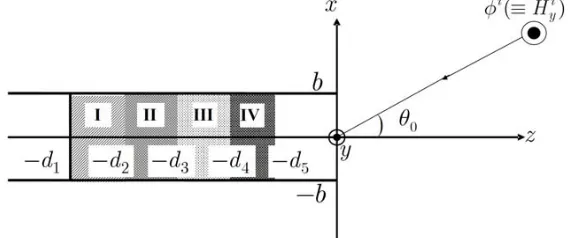
The geometry of the problem is shown in Fig. 1, where the waveguide plates are infinitely thin, perfectly conducting, and uniform in the y -direction. The material layers I (−d1 < z < −d2), II (−d2 < z <

−d3), III(−d3< z <−d4), and IV (−d4 < z <−d5) are characterized

by the relative permittivity/permeability (εm, µm) form= 1,2,3,and

4, respectively.

Figure 1. Geometry of the problem.

Let the total magnetic fieldφt(x, z)≡H_yt(x, z)be

φt(x, z) =φi(x, z) +φ(x, z), (1)

whereφi(x, z) is the incident field of H polarization defined by

φi(x, z) =e−ik(xsinθ0+zcosθ0)_{, 0< θ}

0 < π/2, (2)

wherek[≡ω(µ0ε0)1/2] is the free-space wavenumber. We shall assume

that the vacuum is slightly lossy as ink=k1+ik2 with 0< k2 k1.

The total fieldφt(x, z) satisfies the 2-D Helmholtz equation

where

µ(x, z) =

        

µ1(layer I) µ2(layer II) µ3(layer III) µ4(layer IV)

1 (otherwise)

, ε(x, z) =

        

ε1(layer I) ε2(layer II) ε3(layer III) ε4(layer IV)

1 (otherwise)

. (4)

Once the solution of (3) has been found, nonzero components of the total electromagnetic fields are derived from

H_yt, E_xt, E_zt =

φt, 1 iωε0ε(x, z)

∂φt ∂z ,

i ωε0ε(x, z)

∂φt ∂x

. (5)

It follows from the radiation condition that

φ(x, z) = O

ek2zcosθ0

asz→ −∞,

= O

e−k2z

asz→ ∞. (6)

Let us define the Fourier transform of the scattered field as

Φ(x, α) = (2π)−1/2

_∞

−∞

φ(x, z)eiαzdz,

α = Reα+iImα(≡σ+iτ). (7)

Introducing the Fourier integrals as

Φ+(x, α) = (2π)−1/2

_∞

0

φ(x, z)eiαzdz, (8)

Φ₋(x, α) = (2π)−1/2

d1

−∞φ(x, z)e

iαz_{dz, (9)}

Φ(m)₁ (x, α) = (2π)−1/2

₋dm+1

−dm

φt(x, z)eiαzdz

form= 1,2,3,4, (10)

Φ(5)₁ (x, α) = (2π)−1/2

0

−d5

φt(x, z)eiαzdz, (11)

we can express Φ(x, α) as

Φ(x, α) = Ψ₍₊₎(x, α) + Φ₋(x, α) for |x|> b,

by using (8)–(11), where

Ψ₍₊₎(x, α) = Φ+(x, α)−

e−ikxsinθ0

(2π)1/2_i(α−_kcosθ 0)

, (13)

Φ1(x, α) = 5

m=1

Φ(m)₁ (x, α). (14)

In view of the radiation condition, it follows that Φ(x, α), Φ+(x, α),

and Φ₋(x, α) are regular in −k2 < τ < k2cosθ0, τ > −k2, and τ < k2cosθ0, respectively, whereas Φ(m)1 (x, α) for m = 1,2,3,4,5are

entire functions. We also note that Ψ₍₊₎(x, α) is regular in τ > −k2

except for a simple pole atα=kcosθ0. We shall henceforth use these

conventions for indicating the regions of regularity of functions in the complexα-plane.

Taking the Fourier transform and the Fourier integrations of (3) and solving the resultant equations by following a procedure similar to that developed in [27], we derive a scattered field representation in the Fourier transform domain with the result that

Φ(x, α) = −Ψ₍₊₎(±b, α)γ−1e∓γ(x∓b) for x≷±b,

= Ψ₍₊₎(b, α)coshγ(x+b)

γsinh 2γb

−Ψ₍₊₎(−b, α)coshγ(x−b)

γsinh 2γb

−1 b ∞ n=0 νn

c5n(α) α2_+γ2

n

cosnπ

2b(x+b)

−1 b 4 m=1 ∞ n=0 νn

cmn(α) α2_{+ Γ}2

mn

cosnπ

2b(x+b)

for|x|< b, (15)

whereγ = (α2−k2)1/2 with Reγ >0, and

νn = 1/2 forn= 0,

= 1 for n≥1, (16)

γn = −ik forn= 0,

= (nπ/2b)2−k21/2 forn≥1, (17) Γmn = −ikm forn= 0,

km = (µmεm)1/2k form= 1,2,3,4, (19)

cmn(α) = e−iαdmc+mn(α)−e−iαdm+1c−(m+1)n(α)

form= 1,2,3,4, (20)

c5n(α) = e−iαd5c−5n(α), (21)

c+_1n(α) = f_n+, c−_2n(α) =f1n−iαg1n, (22) c+_2n(α) = (ε2/ε1)f1n−iαg1n, c−3n(α) =f2n−iαg2n, (23) c+_3n(α) = (ε3/ε2)f2n−iαg2n, c−_4n(α) =f3n−iαg3n, (24) c+_4n(α) = (ε4/ε3)f3n−iαg3n, c−5n(α) =f4n−iαg4n. (25)

In (15), the prime denotes differentiation with respect to x. Equation (15) is the scattered field expression in the transform domain. The coefficientsf_n+, fmn, andgmnin (22)–(25) are defined in

Appendix A.

We now differentiate (15) with respect toxand setx=b±0,−b±0 in the results. Making use of the boundary conditions, we obtain that

J₋d(α)=−U(+)(α)

M(α) − 2 b ∞ n=1,odd

c5n(α) α2_+γ2

n

+

4

m=1

cmn(α) α2_{+ Γ}2

mn

, (26)

J₋s(α)=−V(+)(α)

N(α) + 2 b ∞ n=0,even νn

c5n(α) α2_+γ2

n

+

4

m=1

cmn(α) α2_{+ Γ}2

mn

, (27)

where

U₍₊₎(α) = Ψ₍₊₎(b, α) + Ψ₍₊₎(−b, α), (28)

V₍₊₎(α) = Ψ₍₊₎(b, α)−Ψ₍₊₎(−b, α), (29)

J₋d,s(α) = J₋(b, α)∓J₋(−b, α), (30)

J₋(±b, α) = Φ₋(±b±0, α)−Φ1(±b∓0, α), (31) M(α) = γe−γbcoshγb, N(α) =γe−γbsinhγb. (32) Equations (26) and (27) are the desired, simultaneous Wiener-Hopf equations, whereM(α) andN(α) are kernel functions.

3. SOLUTION OF THE WIENER-HOPF EQUATIONS The kernel functions are factorized as [12, 13]

where

M+(α)[=M−(−α)] = (coskb)1/2ei3π/4

·(k+α)1/2exp{(iγb/π) ln [(α−γ)/k]}

·exp{(iαb/π) [1−C+ ln(π/2kb) +iπ/2]}

· ∞

n=1,odd

(1 +α/iγn)e2iαb/nπ, (34)

N+(α)[=N−(−α)] = (ksinkb)1/2exp(iπ/2)

·exp{(iγb/k) ln[(α−γ)/k]}

·exp{(iαb/π) [1−C+ ln(2π/kb) +iπ/2]}

·(1 +α/iγ0)

∞

n=2,even

(1 +α/iγn)e2iαb/nπ (35)

withC(= 0.57721566· · ·) being Euler’s constant.

We multiply both sides of (26) and (27) by M₋(α) and N₋(α), respectively, and decompose the results with the aid of the edge condition. After some manipulations, we arrive at

U₍₊₎(α)=b1/2M+(α)

− A

b(α−kcosθ0) −

∞

n=1

δ2n−1anpnun b(α+iγ2n−1)

, (36)

V(+)(α)=b1/2N+(α)

B

b(α−kcosθ0)−

∞

n=1

ν2n₋2δ2n₋2bnqnvn b(α+iγ2n−2)

, (37)

whereδn is defined by (A20) in Appendix A, and

an = (biγ2n−1)−1, bn= (biγ2n−2)−1, (38) pn = b1/2M+(iγ2n−1), qn= b1/2N+(iγ2n−2), (39) u+_n = U₍₊₎(iγ2n−1), vn+=V(+)(iγ2n−2), (40)

A = −

2b π

1/2

ksinθ0cos(kbsinθ0) M+(kcosθ0)

, (41)

B = −

2b π

1/2

iksinθ0sin(kbsinθ0) N+(kcosθ0)

. (42)

Equations (36) and (37) are the exact solutions to the Wiener-Hopf equations (26) and (27), respectively.

Taking into account the edge condition, we find that

as n → ∞, where Ku and Ku are unknown constants. Approximate

expressions of (36) and (37) are derived by using (43) as

U₍₊₎(α) ≈ b1/2M+(α)

− A

b(α−kcosθ0)

−

N−1

n=1

δ2n−1anpnu+n b(α+iγ2n−1)−

KuSu(α)

, (44)

V(+)(α) ≈ b1/2N+(α)

B b(α−kcosθ0)

−

N−1

n=1

ν2n−2δ2n−2bnqnvn+ b(α+iγ2n−2) −

KvSv(α)

(45)

withN being a large positive integer, where

Su(α) =

∞

n=N

δ2n−1(bγ2n−1)−1 b(α+iγ2n₋1)

, (46)

Sv(α) =

∞

n=N

δ2n−2(bγ2n−2)−1 b(α+iγ2n−2)

. (47)

The unknowns u+_n andv_n+ forn= 1,2,3, . . . , N −1 as well asKu and Kv are involved in (44) and (45), which can be determined by solving

two sets ofN×N matrix equations numerically (see discussion in [27]).

4. SCATTERED FIELD

The scattered field in the real space can be derived by taking the inverse Fourier transform of (15) according to the formula

φ(x, z) = (2π)−1/2

_∞+ic

−∞+ic

Φ(x, α)e−iαzdα,

−k2< c < k2cosθ0. (48)

Substituting (15) into (48) and evaluating the resultant integral for

|x| < b with the aid of (36) and (37), the scattered field inside the waveguide is derived as

φ(x, z) = −φi(x, z) + ∞

n=0

T1ncosh Γ1n(z+d1) cos nπ

2b(x+b)

= −φi(x, z) + ∞

n=0

T_mn− eΓmn(z+dm+1)−_T+

mne−Γmn(z+dm+1)

·cosnπ

2b(x+b) for −dm< z <−dm+1(m= 2,3,4),

= −φi(x, z) + ∞

n=0

T_n−eγn(z+d5)−_T+

ne−γn(z+d5)

·cosnπ

2b(x+b) for −d5< z <0, (49)

where

T1n =

_π

2

1/2_νne−γnd5_e−Γ1n(d1−d2)_P

1nU(+)(iγn) bΓ1n

for oddn,

= −

_π

2

1/2 _νne−γnd5_e−Γ1n(d1−d2)_P

1nV(+)(iγn) bΓ1n

for evenn, (50)

T_mn− = −

_π

2

1/2 νne−γnd5PmnU(+)(iγn) bΓmn

for oddn(m= 2,3,4),

=

_π

2

1/2νne−γnd5PmnV(+)(iγn) bΓmn

for evenn(m= 2,3,4), (51)

T_mn+ = −

_π

2

1/2 νne−γnd5QmnU(+)(iγn) bΓmn

for odd n(m= 2,3,4),

=

_π

2

1/2νne−γnd5QmnV(+)(iγn) bΓmn

for even n(m= 2,3,4), (52)

T_n− = −

_π

2

1/2 νne−γnd5U(+)(iγn) bγn

for odd n,

=

_π

2

1/2νne−γnd5V(+)(iγn) bγn

for even n, (53)

T_n+ = −

_π

2

1/2 νne−γnd5Q4nU(+)(iγn) bγn

=

_π

2

1/2νne−γnd5Q4nV(+)(iγn) bγn

for evenn, (54)

In (50)–(54), Pmn and Qmn for m = 1,2,3, and 4 are defined in

Appendix A.

Next we shall consider the field outside the waveguide and derive a scattered far field for |x|> b. In view of (15), (28), (29), and (48), an integral representation of the scattered field for x≷±b is given by

φ(x, z) = ∓(2π)−1/2

_∞+ic

−∞+ic

γ−1Ψ₍₊₎(±b, α)e−iαzdα,

−k2< c < k2cosθ0, (55)

where

Ψ₍₊₎(±b, α) = U(+)(α)± V(+)(α)

2 . (56)

In order to evaluate (55), we expressφ(x, z) as in

φ(x, z) =φ1(x, z) +φ2(x, z), (57)

where

φ1(x, z) = ±(2π)−1/2

_∞+ic

−∞+ic

γ−1[Ψ₍₊₎(±b, α)

−_Φ(˜ _{±b, α)]e}∓γ(x_∓b)₋iαz_{dα, (58)}

φ2(x, z) = ∓(2π)−1/2

_∞+ic

−∞+ic

γ−1Φ(˜ ±b, α)e∓γ(x∓b)−iαzdα (59)

forx≷±bwith

˜

Φ(±b, α) = ksinθ0e

∓ikbsinθ0_(α+k)1/2

(2π)1/2_(k+kcosθ

0)1/2(α−kcosθ0)

. (60)

For convenience, we now introduce the cylindrical coordinates (ρ1,2, θ1,2) centered at the waveguide edges (x, z) = (±b,0) as follows:

x−b = ρ1sinθ1, z=ρ1cosθ1 for 0< θ1 < π, (61) x+b = ρ2sinθ2, z=ρ2cosθ2 for −π < θ2<0. (62)

In (57), φ1(x, z) is evaluated asymptotically for large |k|ρ1,2 with the

leading to the Fresnel integral representation. Omitting the details, we arrive at the asymptotic expression of (57) with the result that

φ(ρ1,2, θ1,2)

∼ ±Ψ₍₊₎(±b,−kcosθ1,2)−Φ(˜ ±b,−kcosθ1,2)

_ei(kρ1,2−3π/4)

(kρ1,2)1/2

−e∓ikbsinθ0

e−ikρ1,2cos(θ1,2−θ0)_F

(2kρ1,2)1/2cos

θ1,2−θ0

2

−e−ikρ1,2cos(θ1,2+θ0)_F

(2kρ1,2)1/2cos

θ1,2+θ0

2

(63)

askρ1,2 → ∞forx≷±b, whereF(·) is the Fresnel integral defined by

F(w) = e −iπ/4 π1/2

_∞

w

eit2dt. (64)

Equation (63) gives a scattered far field expression uniformly valid in observation anglesθ1,2.

An alternative asymptotic expression of (55) can be derived by using the cylindrical coordinate at the origin

x=ρsinθ, z =ρcosθ for −π < θ < π (65)

and applying the saddle point method. This yields,

φ(ρ, θ)∼φg(ρ, θ) +φd(ρ, θ) (66)

as|k|ρ→ ∞forθnot too close to±π∓θ0, whereφg(ρ, θ) andφd(ρ, θ)

are the geometrical optics field and the diffracted field, respectively, which are defined by

φg(ρ, θ) = −e−ikρcos(θ−θ0) for −π < θ2<−π+θ0,

= 0 for −π+θ0 < θ2<0, 0< θ1 < π−θ0,

= e−2ikbsinθ0_e−ikρcos(θ+θ0) _forπ−_θ

0 < θ1 < π, (67)

φd(ρ, θ) = ±Ψ(+)(±b,−kcosθ)e∓

ikbsinθei(kρ−3π/4)

(kρ)1/2 , θ≷0. (68)

Equation (66) is a non-uniform asymptotic expression of the scattered far field.

5. NUMERICAL RESULTS AND DISCUSSION

in detail. Since the cross section of the waveguide geometry under consideration is of infinite extent, the RCS per unit length is defined by

σ= lim

ρ→∞

2πρ|φ d_|2

|φi|2

, (69)

whereφi andφdare the incident field and the diffracted field given by (2)and (68), respectively. For real k, (69) is simplified by using (28) and (29) as

σ= λ

2U(+)(−kcosθ)±V(+)(−kcosθ)

2

(70)

forθ≷0 with λbeing the free-space wavelength.

Figures 2–5show the normalized monostatic RCS σ/λ as a function of incidence angle θ0, where the values of σ/λ are plotted

in decibels [dB] by computing 10 log₁₀σ/λ. In order to enable comparison between two different polarizations, we have chosen the same parameters as in the E-polarized case analyzed in [27]. The normalized waveguide aperture widthkband the waveguide dimension ratio d1/2b are taken as kb = 3.14, 15.7, 31.4 and d1/2b = 1.0, 3.0,

respectively. In numerical computation, we have chosen ferrite (single-layer material) [1] for region IV and Emerson & Cuming AN-73 (three-layer material) [1] for regions I-III to form the existing four-(three-layer material loaded on the planar termination inside the waveguide (see Fig. 1). The material constants for ferrite and Emerson & Cuming AN-73 areε4 = 2.4 +i1.25, µ4= 1.6 +i0.9 andε1 = 3.14 +i10.0, µ1 =

1.0, ε2= 1.6 +i0.9, µ2= 1.0, ε3= 1.4 +i0.35, µ3 = 1.0, respectively,

where the thickness of the three layers of Emerson & Cuming AN-73 and ferrite is such thatd1−d2=d2−d3 =d3−d4 =d4−d5(= ∆). The

Figure 2(a). Monostatic RCS σ/λ [dB] for d1/2b = 1.0, kb =

3.14, k∆ = 0.628. : cavity with no loading (regions I-IV: vacuum). : cavity with single-layer loading (region I: ferrite, regions II-IV: vacuum). : cavity with three-layer loading (regions I-III: Emerson & Cuming AN-73, region IV: vacuum). : cavity with four-layer loading (regions I-III: Emerson & Cuming AN-73, region IV: ferrite).

Figure 2(b). Monostatic RCS σ/λ [dB] for d1/2b = 1.0, kb =

Figure 2(c). Monostatic RCS σ/λ [dB] for d1/2b = 1.0, kb =

31.4, k∆ = 0.628. Other particulars are the same as in Fig. 2(a).

Figure 3(a). Monostatic RCS σ/λ [dB] for d1/2b = 3.0, kb =

Figure 3(b). Monostatic RCS σ/λ [dB] for d1/2b = 3.0, kb =

15.7, k∆ = 0.628. Other particulars are the same as in Fig. 2(a).

Figure 3(c). Monostatic RCS σ/λ [dB] for d1/2b = 3.0, kb =

Figure 4(a). Monostatic RCS σ/λ [dB] for d1/2b = 1.0, kb =

3.14, k∆ = 1.255. : cavity with no loading (regions I-IV: vacuum). : cavity with single-layer loading (region I: ferrite, regions II-IV: vacuum). : cavity with three-layer loading (regions I-III: Emerson & Cuming AN-73, region IV: vacuum). : cavity with four-layer loading (regions I-III: Emerson & Cuming AN-73, region IV: ferrite).

Figure 4(b). Monostatic RCS σ/λ [dB] for d1/2b = 1.0, kb =

Figure 4(c). Monostatic RCS σ/λ [dB] for d1/2b = 1.0, kb =

31.4, k∆ = 1.255. Other particulars are the same as in Fig. 4(a).

Figure 5(a). Monostatic RCS σ/λ [dB] for d1/2b = 3.0, kb =

Figure 5(b). Monostatic RCS σ/λ [dB] for d1/2b = 3.0, kb =

15.7, k∆ = 1.255. Other particulars are the same as in Fig. 4(a).

Figure 5(c). Monostatic RCS σ/λ [dB] for d1/2b = 3.0, kb =

results for material-loaded cavities between the single- and four-layer cases, it is found that the RCS reduction is more significant in the four-layer case. Similarly by comparing the results for the four-layer case with those for the three-layer case, more RCS reduction is seen in the four-layer case. From these characteristics, it is expected that the multi-layer loading gives rise to better RCS reduction over a broad frequency range.

Let us now make comparisons of the monostatic RCS results between two different polarizations. As mentioned earlier, we have analyzed theE-polarized plane wave diffraction by the same waveguide in our previous paper [27]. Comparing the RCS curves in Figs. 2–5for theHpolarization with those in Figs. 2–5in [27] for theEpolarization, we see differences in all numerical examples. In particular, the monostatic RCS for theHpolarization oscillates rapidly in comparison to the E-polarized case. This difference is due to the fact that the effect of edge diffraction depends on the incident polarization. We also see that, if the waveguide aperture opening is small as in kb = 3.14, there are great differences in the RCS characteristics between the H

polarization (Figs. 2–5in this paper) and theE polarization (Figs. 2–5 in [27]). This is because the diffraction phenomena at low frequencies strongly depend on the incident polarization. It is also found that, with an increase of the waveguide aperture opening, the RCS forEand

H polarizations exhibits close features to each other. Comparing the results betweenk∆ = 0.628 and 1.255, the RCS reduction is noticeable with an increase of the material thickness for both polarizations.

6. CONCLUSIONS

different polarizations have also been made.

APPENDIX A. ON THE COEFFICIENTS f_n+, fmn, AND gmn FOR n= 1,2,3, . . . WITH m= 1,2,3,4 IN (22)–(25) The coefficientsf_n+,fmnand gmnforn= 1,2,3, . . . withm= 1,2,3,4

have appeared in the scattered field expression (15) (see (22)–(25)). These are given as

f_n+ = nπ 2be

−Γ1n(d1−d2)_e−γnd5_P

1nU(+)(iγn) for oddn,

= −nπ 2be

−Γ1n(d1−d2)_e−γnd5_P

1nV(+)(iγn) for evenn, (A1)

fmn = nπ

2bPmnU(+)(iγn) for oddn,

= −nπ

2bPmnV(+)(iγn) for evenn, (A2) gmn =

nπ

2bQmnU(+)(iγn) for odd n,

= −nπ

2bQmnV(+)(iγn) for evenn, (A3)

wherePmn and Qmn are defined by

P4n=

(1 +ρ4n)

1−e−2Γ4n(d4−d5)_ρ 3n

ρ4n

1−e2Γ4n(d4−d5)_ρ3nρ4n

Γ4nε4 γnε4+ Γ4n

, (A4)

Q4n=

e−2Γ4n(d4−d5)_ρ

3n−ρ4n

1−e−2Γ4n(d4−d5)_ρ 3nρ4n

, (A5)

P3n=

(1−ρ4n)e−Γ4n(d4−d5)

1−e−2Γ4n(d4−d5)ρ_3nρ_4n

(1 +δ2n) Γ3nε4

(ε4/ε3) Γ3n+δ2nΓ4n

, (A6)

Q3n=

e−Γ4n(d4−d5)_ρ

3n(1−ρ4n)ε4Γ3n

1−e−2Γ4n(d4−d5)_ρ3nρ4n , (A7) P2n=

(1 +δ1n) Γ2ne−Γ3n(d3−d4)

(ε3/ε2) Γ2n+δ1nΓ3n

· (1−ρ4n)e−Γ4n(d4−d5)

1−e−2Γ4n(d4−d5)_ρ 3nρ4n

(1 +δ2n) Γ3nε4

(ε4/ε3) Γ3n+δ2nΓ4n

, (A8)

Q2n=

e−Γ3n(d3−d4)_ρ

2ne−Γ4n(d4−d5)(1−ρ4n)

1−e−2Γ4n(d4−d5)_ρ 3nρ4n

ε4Γ3n

(ε4/ε3) Γ3n+δ2nΓ4n

P1n=

(Kn+ Γ1n)e−Γ2n(d2−d3)

(ε2/ε1)Kn+ Γ2n

(1 +δ1n) Γ2ne−Γ3n(d3−d4)

(ε3/ε2) Γ2n+δ1nΓ3n

· (1−ρ4n)e−Γ4n(d4−d5)

1−e−2Γ4n(d4−d5)_ρ 3nρ4n

(1 +δ2n) Γ3nε4

(ε4/ε3) Γ3n+δ2nΓ4n

, (A10)

Q1n=

e−Γ2n(d2−d3)_ρ

1n(1 +δ1n) Γ2n

(ε2/ε1) Γ2n+δ1nΓ3n

·e−Γ3n(d3−d4)e−Γ4n(d4−d5)(1−δ3n)

1−e−2Γ4n(d4−d5)_ρ3nρ4n

ε4Γ3n

(ε4/ε3) Γ3n+δ2nΓ4n

, (A11)

where

Kn =

Γ1n+e−2Γ1n(d1−d2)

1−e−2Γ1n(d1−d2) , (A12) ρ1n =

(ε2/ε1)Kn−Γ2n

(ε2/ε1)Kn+ Γ2n

, (A13)

δ1n =

1−ρ1ne−2Γ2n(d2−d3)

1 +ρ1ne−2Γ2n(d2−d3)

, (A14)

ρ2n =

(ε3/ε2) Γ2n−δ1nΓ3n

(ε3/ε2) Γ2n+δ1nΓ3n

, (A15)

δ2n =

1−ρ2ne−2Γ3n(d3−d4)

1 +ρ2ne−2Γ3n(d3−d4)

, (A16)

ρ3n =

(ε4/ε3) Γ3n−δ2nΓ4n

(ε4/ε3) Γ3n+δ2nΓ4n

, (A17)

ρ4n =

ε4γn−Γ4n ε4γn+ Γ4n

. (A18)

Substituting (A2) and (A3) withm= 4 into (21) and settingα=−iγn,

we also find that

c5n(−iγn) = nπ

2bδnU(+)(iγn) for oddn,

= −nπ

2bδnV(+)(iγn) for evenn, (A19)

where

δn=

ρ3ne−2Γ4n(d4−d5)−ρ4n

e−2γnd5

1−ρ3nρ4ne−2Γ4n(d4−d5)

REFERENCES

1. Lee, S.-W. and H. Ling, “Data book for cavity RCS: Version 1,” Tech. Rep., No. SWL 89-1, Univ. Illinois, Urbana, 1989.

2. Lee, S.-W. and R. J. Marhefka, “Data book of high-frequency RCS: Version 2,” Tech. Rep., Univ. Illinois, Urbana, 1989. 3. Stone, W. R., Ed., Radar Cross Sections of Complex Objects,

IEEE Press, New York, 1990.

4. Bernard, J. M. L., G. Pelosi, and P. Ya. Ufimtsev, Eds.,

Special Issue on Radar Cross Section of Complex Objects, Ann. Telecommun., Vol. 50, No. 5–6, 1995.

5. Lee, C. S. and S.-W. Lee, “RCS of a coated circular waveguide terminated by a perfect conductor,” IEEE Trans. Antennas Propagat., Vol. 35, No. 4, 391–398, 1987.

6. Altinta¸s A., P. H. Pathak, and M. C. Liang, “A selective modal scheme for the analysis of EM coupling into or radiation from large open-ended waveguides,”IEEE Trans. Antennas Propagat., Vol. 36, No. 1, 84–96, 1988.

7. Ling, H., R.-C. Chou, and S.-W. Lee, “Shooting and bouncing rays: Calculating the RCS of an arbitrary shaped cavity,” IEEE Trans. Antennas Propagat., Vol. 37, No. 2, 194–205, 1989.

8. Pathak, P. H. and R. J. Burkholder, “Modal, ray, and beam techniques for analyzing the EM scattering by open-ended waveguide cavities,” IEEE Trans. Antennas Propagat., Vol. 37, No. 5, 635–647, 1989.

9. Pathak, P. H. and R. J. Burkholder, “A reciprocity formulation for the EM scattering by an obstacle within a large open cavity,”

IEEE Trans. Microwave Theory Tech., Vol. 41, No. 4, 702–707, 1993.

10. Lee, R. and T.-T. Chia, “Analysis of electromagnetic scattering from a cavity with a complex termination by means of a hybrid ray-FDTD method,” IEEE Trans. Antennas Propagat., Vol. 41, No. 11, 1560–1569, 1993.

11. Ohnuki, S. and T. Hinata, “Radar cross section of an open-ended rectangular cylinder with an iris inside the cavity,”IEICE Trans. Electron., Vol. E81-C, No. 12, 1875–1880, 1998.

12. Noble, B., Methods Based on the Wiener-Hopf Technique for the Solution of Partial Differential Equations, Pergamon, London, 1958.

14. Kobayashi, K., “Wiener-Hopf and modified residue calculus tech-niques,” Analysis Methods for Electromagnetic Wave Problems, Chap. 8, Yamashita, E., Ed., Artech House, Boston, 1990. 15. B¨uy¨ukaksoy, A., F. Birbir, and E. Erdo˘gan, “Scattering

characteristics of a rectangular groove in a reactive surface,”IEEE Trans. Antennas and Propagat., Vol. 43, No. 12, 1450–1458, 1995. 16. C¸ etiner, B. A., A. B¨uy¨ukaksoy, and F. G¨une¸s, “Diffraction of electromagnetic waves by an open ended parallel plate waveguide cavity with impedance walls,” Progress In Electromagnetics Research, PIER 26, 165–197, 2000.

17. Kobayashi, K. and A. Sawai, “Plane wave diffraction by an open-ended parallel plate waveguide cavity,”Journal of Electromagnetic Waves and Applications, Vol. 6, No. 4, 475–512, 1992.

18. Kobayashi, K., S. Koshikawa, and A. Sawai, “Diffraction by a parallel-plate waveguide cavity with dielectric/ferrite loading: Part I — The case of E polarization,” Progress In Electromagnetics Research, PIER 8, 377–426, 1994.

19. Koshikawa, S. and K. Kobayashi, “Diffraction by a parallel-plate waveguide cavity with dielectric/ferrite loading: Part II — The case of H polarization,” Progress In Electromagnetics Research, PIER 8, 427–458, 1994.

20. Koshikawa, S., T. Momose, and K. Kobayashi, “RCS of a parallel-plate waveguide cavity with three-layer material loading,”IEICE Trans. Electron., Vol. E77-C, No. 9, 1514–1521, 1994.

21. Okada, S., S. Koshikawa, and K. Kobayashi, “Wiener-Hopf analysis of the plane wave diffraction by a finite parallel-plate waveguide with three-layer material loading: Part I — The case of E polarization,” Telecommunications and Radio Engineering, Vol. 58, No. 1&2, 53–65, 2002.

22. Okada, S., S. Koshikawa, and K. Kobayashi, “Wiener-Hopf analysis of the plane wave diffraction by a finite parallel-plate waveguide with three-layer material loading: Part II — The case of H polarization,” Telecommunications and Radio Engineering, Vol. 58, No. 1&2, 66–75, 2002.

23. Zheng, J. P. and K. Kobayashi, “Plane wave diffraction by a finite parallel-plate waveguide with four-layer material loading: Part I — The case of E polarization,” Progress In Electromagnetics Research B, Vol. 6, 1–36, 2008.

25. Koshikawa, S. and K. Kobayashi, “Diffraction by a terminated, semi-infinite parallel-plate waveguide with three-layer material loading,” IEEE Trans. Antennas and Propagat., Vol. 45, No. 6, 949–959, 1997.

26. Koshikawa, S. and K. Kobayashi, “Diffraction by a terminated, semi-infinite parallel-plate waveguide with three-layer material loading; the case of H polarization,” Electromagnetic Waves &

Electronic Systems, Vol. 5, No. 1, 13–23, 2000.