Numerical Simulation of a Mathematical Model for Cancer Cell Invasion

ISSN:2574 -1241

Numerical Simulation of a Mathematical Model for

Cancer Cell Invasion

Benito JJ

_{, Garcıa A}

_{, Gavete ML}

_{, Gavete L}

_{*, Negreanu M}

_{, Urena F}

_{and Vargas AM}

1_{U.N.E.D, Madrid, Spain}

2_{Universidad Politecnica de Madrid, Madrid, Spain}

3_{Departamento de Analisis Matematico y Matematica Aplicada, UCM, Madrid, Spain}

*Corresponding author: Gavete L, Universidad Politecnica de Madrid, Madrid, Spain

DOI:10.26717/BJSTR.2019.23.003889

Introduction

In this paper we focus on the discretization of a mathematical model describing the process of cells invasion in the surrounding extracellular matrix using a Generalized Finite Difference Method. Chaplain and Lolas in [1,2] developed a mathematical model con-sisting of three partial differential equations describing the evolu-tion in time and space of the system variables. It is assumed that the key physical variables are tumor cell density (denoted by U); protein density of the extracellular matrix (denoted by W) and the concentration of the chemical substance responsible for the che-motaxis (denoted by V) each of them considered at and time t > 0. Throughout this paper _{Ω ⊂R}2 _{is a bounded domain with a regular} boundary. The model is the following:

(1)

where we consider the chemotactic and hepatotactic coeffi -cients, η and ρ, respectively, to be constant and positive. The

pa-natural to assume homogeneous Neumann boundary condition as we assume that invasion takes place within an isolated system (see [2]). We consider for our numerical simulation

(2)

Tao and Winkler in [3] have demonstrated that whenever the initial data (U₀, V₀, W₀) are regular fulfilling

0 o

U > ,Wo≤1and 2 8

K>η _{, solution (U,V,W) converges} asumptoti-cally to the constant stationary solution (1, 1, 0) in the . The GFDM has been recently proved to obtain highly accurate ap-proximations to the solutions of nonlinear PDEs (see for instance [6,5,4]. The paper is organized as follows: in Section 2 we present the explicit formula of the GFDM and obtain the explicit scheme. In Section 3 we present numerical examples. In particular, the first ex -ample shows the convergence of the solution to the constant steady state (1, 1, 0), in accordance with the theory [3]. The second and third examples show that for an appropriate initial data the solu-tion converges to (0, 0, ), with arbitrary. Finally, we obtain some conclusions in Section 4.

Received: November 20, 2019 Published: December 02, 2019

Citation: Benito JJ, Garcıa A, Gavete ML, Gavete L, Negreanu M, Urena F, Vargas AM.Numerical Simulation of a Mathemat-ical Model for Cancer Cell Invasion. Bi-omed J Sci & Tech Res 23(2)-2019. BJSTR. MS.ID.003889.

ARTICLE INFO Abstract

In this paper we analyze a mathematical model of cancer cell invasion consisting of a system of partial differential equations which describes the interactions between cancer cells, the matrix degrading enzyme and the host tissue. The main objective of the present paper is to show, using numerical computations, the ability of a relatively simple model to produce complicated dynamics. We build some novel techniques and numerical algorithms based on the Generalized Finite Difference Method (GFDM) and test the method in several examples.

GFD Scheme

As stated in the introduction, our objective is to derive a discret -ization of system (1) using the GDF explicit formulae. To do so, let us consider a bounded domain Ω ⊂R2. Then,

2 2

2 2 2 2

t U U U V U V U W U W

U

x y η x x η y y ρ x x ρ y y

∂ ∂ ∂ ∂ ∂ ∂ ∂ ∂ ∂ ∂

= + − − − −

∂ ∂ ∂ ∂ ∂ ∂ ∂ ∂ ∂ ∂ ₍₃₎

2 2

2 2 ,

t V V

V V U

x y ∂ ∂ = + − + ∂ ∂ (4) . t

W = −VW (5)

Therefore, system (1) reads as equations (3), (4) and (5) to-gether with the nonnegative initial data

(6)

With 2

0 0 0

0≤U X V X W X( ), ( ), ( )∈C( ),Ω− _{and the boundary conditions}

U V W 0, , )(xt (0, ).

n n n

∂ ₌∂ ₌∂ _{= ∈∂Ω}

∂ ∂ ∂ × ∞ (7) The explicit formulae of the GFD explicit scheme can be seen in [4, 5, 6], although for the sake of completeness we reproduce below

(8)

Where 0 ₁

s j _i ij

ϖ

ϖ

=

= ∑

For j = 0; 1; 2. The time derivative is approximated by

Then, the GFD scheme for the system (3)-(5) is:

(9)

(10) and

(11)

Numerical Computations

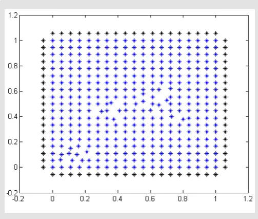
We consider an irregular cloud of points see (Figure 1) model-ling our in vitro domain. For all examples we denote by (u, v, w) the approximate solution given by the GFDM. For all numerical exam-ples we use as time step ∆ =t 0.001 and, then, T (s) (total time) is calculated by n t∆ .

Figure 1: Irregular clouds of points.

Example 1

In this first example we solve numerically system given by (3)-(5). We consider η ρ= =0.5 and k=1.5.

We take into account the following initial data:

(12) As we have mentioned in Section 1, since the assumption κ >

2

8

η

is fulfilled, we expect to find convergence of the solution in the sense

In (Table 1) we present the of the approximate solution for different times. Figure 2 shows the different solutions at such times.

Table 1: Values of u l∞( )_Ω, _{v l}∞_{( )Ω} and _{w l}∞_{( )Ω} for different time values in the Example 1.

T(S) 1 5 10 15 20

( )

u l∞ _Ω

0.0125 0.0759 0.5645 0.9846 0.9999

( )

v l∞ _Ω

0.0800 0.0519 0.4229 0.9494 0.9991

( )

w l∞ _Ω

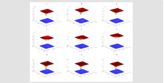
Figure 2: Approximate solution for 1, 10 and 20 seconds for Example 1.

Example 2

For this second case we also consider η ρ= =0.5 _and K=1.5_{. As}

initial data we consider

(13) Notice that W0≤1 does not hold. Then, the assumptions of [3]

are not fulfilled. Table 2 shows the maximum value of the approxi -mate solutions for different times [4]. Figure 3 shows the approxi-mate solutions at 1, 10 and 20 seconds. We obtain convergence to the steady state (0, 0, 1). To the best of our knowledge no analyti-cal proof of this convergence is known [5,6].

Table 2: Values of u l∞( )_Ω , _{v l}∞_{( )Ω and w l}∞_{( )Ω}

for different time values in the Example 2.

T(S) 1 5 10 15 20

( )

u l∞ _Ω

0.0069 0.0043 0.0029 0.0022 0.0019

( )

v l∞ _Ω

0.0060 0.0048 0.0031 0.0023 0.0019

( )

w l∞_Ω

1.0953 1.0706 1.0503 1.0365 1.0257

Example 3

Let us choose now η=0.5_, ρ=0.6 _andK=1.5_{. As initial data we}

consider the following

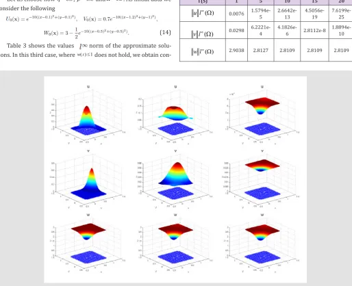
(14) Table 3 shows the values norm of the approximate solu-tions. In this third case, where w( ) 1X ≤ does not hold, we obtain

con-vergence to the steady state (0, 0, 2.8109). In general, this means that solution to (1) converges to

(0,0, )

w

ˆ

where wˆ is an arbitrary function (which seems to depend on 0( )

W X dX Ω

∫ _{). Figure 4 shows the approximate solution of this third} case. Note that we introduce the solutions at small times in order to capture the dynamical complexity of the model.

Table 3: Values of u l∞( )_Ω , _{v l}∞_{( )Ω} and _{w l}∞_{( )Ω for different time}

values in the Example 3.

T(S) 1 5 10 15 20

( )

u l∞ _Ω

0.0076 1.5794e-₅ 2.6642e-₁₃ 4.5056e-₁₉ 7.6199e-₂₅

( )

v l∞ _Ω 0.0298 6.2221e-₄ 4.1826e-₆ 2.8112e-8 1.8894e-₁₀

( )

w l∞ _{Ω 2.9038 2.8127 2.8109 2.8109 2.8109}

Figure 4: Approximate solution for 0, 0.1 and 1 seconds in Example 3.

Conclusion

We have derived the discretization of the chemotaxis-hypotax-is system (1) using a GFD scheme. The dchemotaxis-hypotax-iscrete solution obtained inherits the complicated dynamical behavior of the analytical solu-tion. The Generalized Finite Difference Method solves this strongly coupled highly nonlinear parabolic-elliptic system efficiently and with high accuracy.

Acknowledgement

References

1. Chaplain MA J and Lolas G (2005) Mathematical modelling of cancer

cell invasion of tissue: The role of the urokinase plasminogen activation

system. Mathemat Models Methods Applied Sci 15(11): 1685-1734.

2. Chaplain MA J, Lolas G (2006) Mathematical modelling of cancer cell

invasion of tissue: Dynamic heterogeneity. Networks Heterogenous Media 1(3): 399-439.

3. Tao Y, Winkler M (2015) Large time behavior in a multidimensional chemotaxis-haptotaxis model with slow signal diffusion. Siam J Math

Anal 47(6): 4229-4250.

4. Gavete ML, Vicente F, Gavete L, Urena F, Benito JJ (2019) Numerical simulation in electrocardiology using an explicit Generalized Finite Difference Method. Biomed J Sci & Tech Res13(5).

5. Benito JJ, Urena F, Gavete L (2001) Influence of several factors in the gener- alized finite difference method. Applied Mathemat Model 25:

1039-1053.

6. Urena F, Gavete L, Garcia A, Benito JJ, Vargas AM (2019) Solving second order non-linear parabolic PDEs using generalized finite difference method (GFDM). J Comput Applied Mathemat 354: 221-241.

Submission Link: https://biomedres.us/submit-manuscript.php

Assets of Publishing with us

• Global archiving of articles

• Immediate, unrestricted online access • Rigorous Peer Review Process • Authors Retain Copyrights • Unique DOI for all articles

https://biomedres.us/ This work is licensed under Creative

Commons Attribution 4.0 License

ISSN: 2574-1241