Performance Evaluation of Adaptive Equalization methods and LMS, CMA, FS-CMA Algorithms and Coding for 4-QAM

(1)

IJEDR1703081

International Journal of Engineering Development and Research (

www.ijedr.org

)

546

Performance Evaluation of Adaptive Equalization

methods and LMS, CMA, FS-CMA Algorithms and

Coding for 4-QAM

Jaswant1_{and Dr. Sanjeev Dhull}2 1_{Research Scholar,}2_{Associate Professor,}

Electronics and Communication GJUS & T, Hisar, Haryana, India.

_______________________________________________________________________________________________

Abstract - In this paper a profound evaluation of adaptive equalization technique has been demonstrated. One of the most popular and widely used algorithms i.e. LMS algorithm has been explained in detail. Its successor CMA (Constant Modulus Algorithm), and modified version of CMA i.e. Fractionally Spaced Constant Modulus Algorithm (FS-CMA)[6] have also been incorporated in this text to evaluate comparatively. Simulated results are depicted to show the improved performance due to equalization. All the results have been performed for 4-bit QAM [1] in AWGN and evaluated at 25dB SNR.

Key Words: Adaptive Equalization, QAM, LMS,CMA, FS-CMA.

_______________________________________________________________________________________________

INTRODUCTION

Adaptive Blind equalization[11] has the potential to improve the efficiency of communication systems by eliminating training signals Blind equalizers are used in micro-wave radio. They were realized in Very Large Scale Integration (VLSI) for various purposes. Blind processing applications are emerging in wireless communication technology. Blind methods are of great importance in digital signal communication systems as they allow channel equalization at the receiver without the use of training signals or additional bits. The topic of blind equalization of Linear Time Invariant (LTI) channels, both SIMO and MIMO, has drawn considerable attention over the past years and several algorithms have been developed. One of the practical problems in digital communications is Inter-Symbol Interference (ISI), which causes a given transmitted symbol to be distorted by other transmitted symbols. The ISI is imposed on the transmitted signal due to the band limiting effect of the practical channel and also due to the multipath effects (echo) of the channel [1]. One of the most commonly used techniques to counter channel distortion (ISI) is linear channel equalization. The equalizer is a linear filter that provides an approximate inverse of the channel response. Since it is common for the channel characteristics to be unknown or to change over time, the preferred embodiment of the equalizer is a structure that is adaptive in nature.

Over the period of time, different methods have been developed to counter the effects of ISI and channel distortion. Most popular and most widely used method is Least Mean Square (LMS) algorithm. This method does not give global minima in low SNR (Signal to Noise Ratio). To overcome this drawback, Constant Modulus Algorithms [3],[8] have been developed. In Constant Modulus methods, phase and clock recovery are the challenging problems. So, to overcome these problems modified versions of Constant Modulus methods are used.

ADAPTIVE EQUALIZATION CODING & RESULTS

T=1000; % total number of data

M=500; % total number of training symbols dB=25; % SNR in dB value

%%%%%%%%% Simulate the Received noisy Signal %%%%%%%%%%% N=20; % smoothing length N+1 Lh=5; % channel length = Lh+1 P=round((N+Lh)/2); % equalization delay

h=randn(1,Lh+1)+sqrt(-1)*randn(1,Lh+1); % channel (complex) h=h/norm(h); % normalize

s=round(rand(1,T))*2-1; % QPSK or 4 QAM symbol sequence s=s+sqrt(-1)*(round(rand(1,T))*2-1);

(2)

IJEDR1703081

International Journal of Engineering Development and Research (

www.ijedr.org

)

547

vn=randn(1,T)+j*randn(1,T); % AWGN noise (complex)

vn=vn/norm(vn)*10^(-dB/20)*norm(x); % adjust noise power with SNR dB SNR=20*log10(norm(x)/norm(vn)) % Check SNR of the received samples x=x+vn; % received signal

%%%%%%%%%%%%% channel equalization

Lp=T-N; % remove several first samples to avoid 0 or negative subscript X=zeros(N+1,Lp); % sample vectors (each column is a sample vector)

for i=1:Lp

X(:,i)=x(i+N:-1:i).'; end

hb=zeros(N+1,1); % estimated channel

for i=1:M-10 % need carefully adjust parameter 10 to have positive subscript hb=hb+X(:,i+10)*conj(s(i+10+N-P)); % channel estimation (use all data samples)

end

hb=hb/norm(hb);

%hb=hb(N+1:-1:1)/norm(hb); % normalized channel estimation

%hb1=hb(P-Lh+1:P-Lh+1+Lh).'; hb1=hb1/norm(hb1); % remove zero head and tail (because N>Lh) %Channel_MSE=norm(hb1-h) % estimation error MSE

Rx=zeros(N+1,N+1); % before calculate correlations, initialize for i=1:Lp

Rx=Rx+X(:,i)*X(:,i)'; % calculate correlation matrix end

Rx=Rx/Lp;

f=inv(Rx)*hb; % calculate the MMSE equalizer

sb=f'*X; % estimate symbols (perform equalization)

% calculate SER

sb1=sb/(f'*hb); % scale the output

sb1=sign(real(sb1))+j*sign(imag(sb1)); % perform symbol detection

start=7; % carefully find the corresponding begining point sb2=sb1-s(start+1:start+length(sb1)); % find error symbols

SER=length(find(sb2~=0))/length(sb2) % calculate SER

if 1

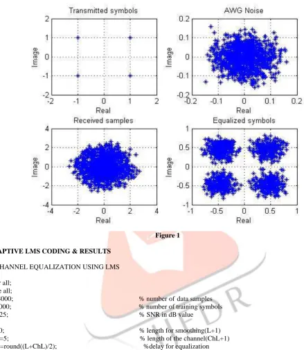
subplot(221),

plot(s,'*'); % show the pattern of transmitted symbols grid,title('Transmitted symbols'); xlabel('Real'),ylabel('Image')

axis([-2 2 -2 2])

subplot(222),

plot(vn,'*'); % show the pattern of AWG noise grid, title('AWG noise'); xlabel('Real'), ylabel('Image')

subplot(223),

plot(x,'*'); % show the pattern of received samples grid, title('Received samples'); xlabel('Real'), ylabel('Image')

subplot(224),

plot(sb,'*'); % show the pattern of the equalized symbols grid, title('Equalized symbols'), xlabel('Real'), ylabel('Image')

(3)

IJEDR1703081

International Journal of Engineering Development and Research (

www.ijedr.org

)

548

Figure 1

ADAPTIVE LMS CODING & RESULTS

% CHANNEL EQUALIZATION USING LMS clc;

clear all; close all;

M=3000; % number of data samples T=2000; % number of training symbols dB=25; % SNR in dB value

L=20; % length for smoothing(L+1) ChL=5; % length of the channel(ChL+1) EqD=round((L+ChL)/2); %delay for equalization

Ch=randn(1,ChL+1)+j*randn(1,ChL+1); % complex channel

Ch=Ch/norm(Ch); % scale the channel with norm

TxS=round(rand(1,M))*2-1; % QPSK transmitted sequence TxS=TxS+sqrt(-1)*(round(rand(1,M))*2-1);

x=filter(Ch,1,TxS); %channel distortion

n=randn(1,M); %+j*randn(1,M); %Additive white gaussian noise

n=n/norm(n)*10^(-dB/20)*norm(x); % scale the noise power in accordance with SNR x=x+n; % received noisy signal

K=M-L; % Discarding several starting samples for avoiding 0's and negative X=zeros(L+1,K); % each vector column is a sample

for i=1:K

(4)

IJEDR1703081

International Journal of Engineering Development and Research (

www.ijedr.org

)

549

%adaptive LMS Equalizer

e=zeros(1,T-10); % initial error c=zeros(L+1,1); % initial condition mu=0.001; % step size for i=1:T-10

e(i)=TxS(i+10+L-EqD)-c'*X(:,i+10); % instant error

c=c+mu*conj(e(i))*X(:,i+10); % update filter or equalizer coefficient end

sb=c'*X; % recieved symbol estimation

%SER(decision part)

sb1=sb/norm(c); % normalize the output

sb1=sign(real(sb1))+j*sign(imag(sb1)); %symbol detection start=7;

sb2=sb1-TxS(start+1:start+length(sb1)); % error detection SER=length(find(sb2~=0))/length(sb2); % SER calculation disp(SER);

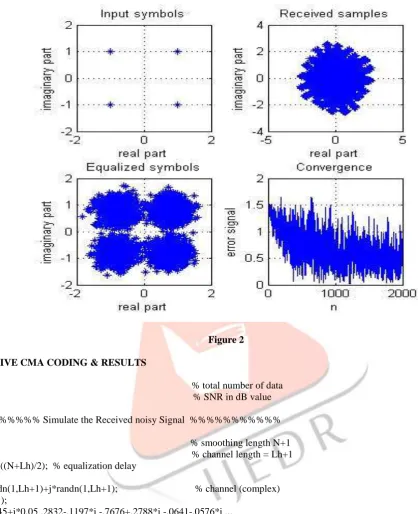
% plot of transmitted symbols subplot(2,2,1),

plot(TxS,'*');

grid,title('Input symbols'); xlabel('real part'),ylabel('imaginary part') axis([-2 2 -2 2])

% plot of received symbols subplot(2,2,2),

plot(x,'*');

grid, title('Received samples'); xlabel('real part'), ylabel('imaginary part')

% plots of the equalized symbols subplot(2,2,3),

plot(sb,'*');

grid, title('Equalized symbols'), xlabel('real part'), ylabel('imaginary part')

% convergence subplot(2,2,4),

plot(abs(e));

(5)

IJEDR1703081

International Journal of Engineering Development and Research (

www.ijedr.org

)

550

Figure 2

ADAPTIVE CMA CODING & RESULTS

T=3000; % total number of data dB=25; % SNR in dB value

%%%%%%%%% Simulate the Received noisy Signal %%%%%%%%%%%

N=20; % smoothing length N+1 Lh=5; % channel length = Lh+1 P=round((N+Lh)/2); % equalization delay

%h=randn(1,Lh+1)+j*randn(1,Lh+1); % channel (complex) j=sqrt(-1);

h=[0.0545+j*0.05 .2832-.1197*j -.7676+.2788*j -.0641-.0576*j ... .0566-.2275*j .4063-.0739*j];

h=h/norm(h); % normalize

s=round(rand(1,T))*2-1; % QPSK or 4 QAM symbol sequence s=s+j*(round(rand(1,T))*2-1);

% generate received noisy signal

x=filter(h,1,s);

vn=randn(1,T)+j*randn(1,T); % AWGN noise (complex)

vn=vn/norm(vn)*10^(-dB/20)*norm(x); % adjust noise power with SNR dB value SNR=20*log10(norm(x)/norm(vn)) % Check SNR of the received samples x=x+vn; % received signal

%%%%%%%%%%%%% adaptive equalizer estimation via CMA

(6)

IJEDR1703081

International Journal of Engineering Development and Research (

www.ijedr.org

)

551

for i=1:Lp

X(:,i)=x(i+N:-1:i).'; end

e=zeros(1,Lp); % used to save instant error f=zeros(N+1,1); f(P)=1; % initial condition

R2=2; % constant modulas of QPSK symbols mu=0.001; % parameter to adjust convergence and steady error for i=1:Lp

e(i)=abs(f'*X(:,i))^2-R2; % instant error f=f-mu*2*e(i)*X(:,i)*X(:,i)'*f; % update equalizer f(P)=1;

% i_e=[i/10000 abs(e(i))] % output information end

% calculate SER

H=zeros(N+1,N+Lh+1); for i=1:N+1, H(i,i:i+Lh)=h; % channel matrix

fh=f'*H; % composite channel+equalizer response should be delta-like temp=find(abs(fh)==max(abs(fh))); % find the max of the composite response

sb1=sb/(fh(temp)); % scale the output

start=6; % carefully find the corresponding begining p oint sb2=sb1-s(start+1:start+length(sb1)); % find error symbols

if 1

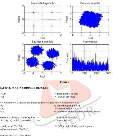
subplot(221),

axis([-2 2 -2 2])

subplot(222),

subplot(223),

subplot(224),

plot(abs(e)); % show the convergence grid, title('Convergence'), xlabel('n'), ylabel('Error e(n)')

(7)

IJEDR1703081

International Journal of Engineering Development and Research (

www.ijedr.org

)

552

Figure 3

ADAPTIVE FS-CMA CODING & RESULTS

T=1000; % total number of data dB=25; % SNR in dB value

%%%%%%%%% Simulate the Received noisy Signal %%%%%%%%%%% N=5; % smoothing length N+1 Lh=5; % channel length = Lh+1

Ap=4; % number of subchannels or receive antenna s

h=randn(Ap,Lh+1)+j*randn(Ap,Lh+1); % channel (complex) for i=1:Ap, h(i,:)=h(i,:)/norm(h(i,:)); end % normalize

s=round(rand(1,T))*2-1; % QPSK or 4 QAM symbol sequence s=s+j*(round(rand(1,T))*2-1);

% generate received noisy signal

x=zeros(Ap,T); % matrix to store samples from Ap antennas SNR=zeros(1,Ap);

for i=1:Ap

x(i,:)=filter(h(i,:),1,s);

vn=randn(1,T)+j*randn(1,T); % AWGN noise (complex) vn=vn/norm(vn)*10^(-dB/20)*norm(x(i,:)); % adjust noise power

SNR(i)=20*log10(norm(x(i,:))/norm(vn)); % Check SNR of the received samples x(i,:)=x(i,:)+vn; % received signal

end

SNR=SNR % display and check SNR

%%%%%%%%%%%%% adaptive equalizer estimation via CMA

Lp=T-N; % remove several first samples to avoid 0 or negative subscript X=zeros((N+1)*Ap,Lp); % sample vectors (each column is a sample vector)

(8)

IJEDR1703081

International Journal of Engineering Development and Research (

www.ijedr.org

)

553

X((j-1)*(N+1)+1:j*(N+1),i)=x(j, i+N:-1:i).';

end end

e=zeros(1,Lp); % used to save instant error f=zeros((N+1)*Ap,1); f(N*Ap/2)=1; % initial condition

R2=2; % constant modulas of QPSK symbols

mu=0.001; % parameter to adjust convergence and steady error for i=1:Lp

e(i)=abs(f'*X(:,i))^2-R2; % instant error f=f-mu*2*e(i)*X(:,i)*X(:,i)'*f; % update equalizer f(N*Ap/2)=1;

% i_e=[i/10000 abs(e(i))] % output information end

% calculate SER

H=zeros((N+1)*Ap,N+Lh+1); temp=0; for j=1:Ap

for i=1:N+1, temp=temp+1; H(temp,i:i+Lh)=h(j,:); end % channel matrix end

fh=f'*H; % composite channel+equalizer response should be delta-like temp=find(abs(fh)==max(abs(fh))); % find the max of the composite response

sb1=sb/(fh(temp)); % scale the output

start=N+1-temp; % general expression for the beginning matching point sb2=sb1(10:length(sb1))-s(start+10:start+length(sb1)); % find error symbols

if 1

subplot(221),

axis([-2 2 -2 2])

subplot(222),

subplot(223),

subplot(224),

plot(abs(e)); % show the convergence grid, title('Convergence'), xlabel('n'), ylabel('Error e(n)')

(9)

IJEDR1703081

International Journal of Engineering Development and Research (

www.ijedr.org

)

554

Figure 4

SIMULATION RESULTS AND CONCLUSION

The coding of adaptive algorithms, LMS, CMA & FS-CMA have been simulated and verified respectively. Results are depicted in Figure 1 to 4. Same AWG noise has been added in all the algorithms to simulate the results. AWG noise has been simulated in Fig.1.Same signal 4-bit QAM and SNR=25dB have been used for all the above algorithms for uniformity. FS-CMS gives improved performance over CMA & LMS in noisy environment.

REFERENCES

1. J.R. Treichler, M.G. Larimore and J.C. Harp, “Practical Blind Demodulators for High- order QAM signals", Proceedings of the IEEE special issue on Blind System Identification and Estimation, vol. 86, pp. 1907-1926, Oct. 1998

2. O. Dabeer, E. Masry, “Convergence Analysis of the Constant Modulus Algorithm,” IEEE Trans. Inform. Theory, vol. 49 , no. 6, Jun. 2003, pp. 1447-1464.

3. D. N. Godard, “Self-recovering equalization and carrier tracking in two dimensional data communication system,” IEEE Trans. Commun., vol. COM-28, no. 11, pp. 1867–1875, Nov. 1980.

4. J. R. Treichler and M. G. Larimore, “New processing techniques based on the constant modulus algorithm,” IEEE Trans. Acoust., Speech, Signal Process., vol. ASSP-33, no. 4, pp. 420–431, Apr. 1985.

5. C. R. Johnson et al., “Blind equalization using the constant modulus criterion: A review,” Proc. IEEE, vol. 86, no. 10, pp. 1927–1950, Oct. 1998.

6. Y. Li and Z. Ding, “Global convergence of fractionally spaced Godard (CMA) adaptive equalizers,” IEEE Trans. Signal Process., vol. 44, no. 4, pp. 818–826, Apr. 1996.

7. Junwen Zhang, Jiajun, Nan Chi, Ze Dong, Jianguo Yu, Xinying Li, Li Tao, and Yufeng Shao,” Multi modulus Blind Equalizations Of QDB spectrum QPSK Digital Signal Processing”, Journel of Light wave technology, vol31,no7 april 2013.

8. P.Rambabu, Rajesh Kumar,”Blind Equalizations using Constnt Modulus Algorithm and Multi modulus algorithm”.Internatinal Journel of computer applications , Vol1, no3.

9. Brown, D.R., P. B. Schniter, and C. R. Johnson, Jr., “Computationally e cient blind equalization,” 35th_{Annual Allerton}

(10)

IJEDR1703081

International Journal of Engineering Development and Research (

www.ijedr.org

)

555

10. Shafayat Abrar and Roy A. Axford Jr.,”Sliced Multi Modulus Algorithm” ETRI Journal, Volume 27, Number 3, June 2005. 11. Ding, Z., R. A. Kennedy, B. D. O. Anderson and C. R. John- son, Jr., “Ill-convergence of godard blind equalizers in data communication systems,” IEEE Trans. On Communications, Vol. 39.

12. Casas, R. A., C. R. Johnson, Jr., R. A. Kennedy, Z. Ding, and R. Malamut, “Blind adaptive decision feedback equalization: A class of channels resulting in illconvergence from a zero initialization,” International Journal on Adaptive Control and Signal Processing Special Issue on Adaptive Channel Equalization.

13. Johnson, Jr., C. R. and B. D. O. Anderson, “Godard blind equalizer error surface characteristics: White, zero mean, binary source case,” International Journal of Adaptive Control and Signal Processing, Vol. 9, 301–324.

14. T. P. Krauss, M. D. Zoltowski, and G. Leus : ‘Simple MMSE equalizers for CDMA downlink to restore chip sequence : Comparison toZero-Forcing and Rake’, ICASSP, May 2000, Vol. 5, pp.2865- 2868.