Multi‑method approach to wellness
predictive modeling
Ankur Agarwal
1, Christopher Baechle
1, Ravi S. Behara
2*and Vinaya Rao
3Introduction
Wellness
Wellness is the proactive process of being aware of one’s lifestyle and making choices to attain a healthy fulfilling life. Good health is a gift that is sometimes taken for granted and is difficult to regain after it has been lost. Maintaining a healthy lifestyle is easier than fighting chronic illness while trying to become healthy. In this paper, we look to use recent advances in data mining to help doctors and patients assess lifestyle choices and overall health to create a wellness score. Data collected by the Centers for Disease Con-trol is analyzed and the wellness of over 5000 patients is modeled. Modeling techniques are then aggregated to maximize the predictive power of the wellness score.
Perception of personal wellness is influenced by culture and values. This research uses the term wellness as defined by Anspaugh et al. [1] which outlines seven different com-ponents which define wellness: physical, spiritual, intellectual, occupational, environ-mental, social and emotional. See Fig. 1. Each component is interrelated and changing one may have an effect on others. A healthy lifestyle plays a major role in optimizing the
Abstract
Patient wellness and preventative care are increasingly becoming a concern for many patients, employers, and healthcare professionals. The federal government has increased spending for wellness alongside new legislation which gives employers and insurance providers some new tools for encouraging preventative care. Not all preventative care and wellness programs have a net positive savings however. Our research attempts to create a patient wellness score which integrates many lifestyle components and a holistic patient prospective. Using a large comprehensive survey conducted by the Centers for Disease Control and Prevention, models are built com-bining both medical professional input and machine learning algorithms. Models are compared and 8 out of 9 models are shown to have a statistically significant (p = 0.05) increase in area under the receiver operating characteristic when using the hybrid approach when compared to expert-only models. Models are then aggregated and lin-early transformed for patient-friendly output. The resulting predictive models provide patients and healthcare providers a comprehensive numerical assessment of a patient’s health, which may be used to track patient wellness so at to help maintain or improve their current condition.
Keywords: Decision support system, Wellness, Data mining, NHANES 2011–2012, Feature selection
Open Access
© 2016 The Author(s). This article is distributed under the terms of the Creative Commons Attribution 4.0 International License (http://creativecommons.org/licenses/by/4.0/), which permits unrestricted use, distribution, and reproduction in any medium, provided you give appropriate credit to the original author(s) and the source, provide a link to the Creative Commons license, and indicate if changes were made.
RESEARCH
*Correspondence: [email protected] 2 Department of IT and Operations Management, College of Business, Florida Atlantic University, Boca Raton, FL, USA
holistic picture of wellness. Modeling can be utilized to assist patients in realizing the impact their lifestyle choices have upon their health.
Financial impact
The United States spends more on healthcare than any other nation. In 2013 the United States spent 17.1 % of its gross domestic product (GDP) on healthcare. The next larg-est spender, France, spent 11.6 % of their GDP on healthcare. The average US resident spent $1047 in out-of-pocket expenses during that same year [2]. Those large healthcare costs do not translate into healthier residents. A 2014 study found that 68 % of Ameri-cans aged 65 and older had 2 chronic conditions. This does not fare well when compared with other industrialized countries, ranging from 33 % in the United Kingdom to 56 % in Canada [3].
Wellness is an important factor in workplace costs and productivity as well. Employers often provide healthcare benefits for employees and these benefits have become increas-ingly expensive. According to industry consultant AON Hewitt, in 2015 the average US employer spent $8640 per employee in direct healthcare related expenses and has stead-ily increased since at least 2010 [4]. Many employers have chosen to offset these costs by increasing the share of employee contributions from an average of $3389 in 2010 to
$5151 in 2015, representing a 52 % increase. Indirect health care expenses are also costly. According to the CDC, losses due to indirect health related issues such as absenteeism or reduced work output from poor health can often be larger than direct medical costs [5]. Changing demographics are projected to exacerbate the problem. In 2000 13 % of US workers were 55 and older. Estimates show this will increase to 25 % of workers by 2020 [6].
Regulatory changes
The Patient Protection and Affordable Care Act (ACA) is a federal statue signed into law in 2010. The act has many new sweeping regulations aimed at increasing the quality of healthcare while addressing rising healthcare costs. Under the ACA, many new proac-tive health measures are now available to patients. Annual wellness visits with healthcare professionals are now available to patients with medical insurance [7]. These visits are free to patients even if yearly deductibles have not been met. This is a major shift from traditional coverage plans which focused on reactionary care rather than preventative care.
Many of the ACA’s new rules support workplace wellness programs as well. Employers are now allowed to give financial incentives to workers participating in most programs. Programs are categorized into (1) participation based and (2) outcome based programs. Examples of participation based programs are gym memberships or completion of a cholesterol screening. Examples of outcome based programs are meeting a target blood pressure or lowering body mass index (BMI).
Wellness score
With so many regulatory changes and increasing pressure to reduce healthcare costs, it should be apparent that wellness has quickly become a priority for patients, medical pro-fessionals, insurance companies, and the federal government. Measuring wellness and predicting chronic disease is an important piece to the larger system. Without accurate measurement and assessment, patients cannot methodically track progress and deter-mine their risk.
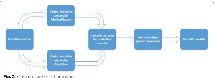
We address this with the creation of a wellness score. Figure 2 outlines our frame-work. The score is designed to integrate a large number of variables while being sim-ple for patients to comprehend. Our work attempts to use a hybrid approach to variable
selection composing of both medical expert analysis and machine learning models. The dataset used to create the models is a large national health survey funded by the United States federal government. Models are then aggregated to create a single score aimed at being simple and patient-friendly.
Background
Effectiveness and costs of current preventative methods
The costs and logistics of preventative care cannot be understated. Unfocused preventa-tive screenings can cost more than the illness they intend to mitigate. Secondary preven-tative services such as mammograms and depression screenings result in a net loss of $2 billion [8]. For example, low dose computed tomography scans for screening of lung cancer have been shown to increase lifespan. However, the small increase in lifespan has not warranted the cost of large scale implementations outside of clinical trial settings [9]. Not all preventative care results in a net financial loss. Primary preventative services such as daily aspirin regimens and alcohol and tobacco screenings result in a net savings of $1.5 billion [8].
Risk factors may dictate which screenings are cost effective. HIV screenings are cost effective in medium to high risk groups, but are not cost effective in low risk groups [10]. Wealthy individuals able to pay for unfocused screenings while asymptomatic may feel the cost is worthwhile if it is able to expand their life span by a small amount. However research shows that these types of screenings have no correlation with increased lifespan and false positives may result in additional invasive tests [11]. Clearly there is a need for systems which can determine an individual’s overall wellness without a litany of expen-sive screenings.
National Health and Nutrition Examination Survey
The National Health and Nutrition Examination Survey (NHANES) was first conducted in 1971 by the National Center for Health Statistics (NCHS) to assess the health, illness, and nutritional status of those living in the United States [12]. The survey was unique in its goal to rigorously examine a large number of people. Such a large undertaking had not been successful up to that point. While NHANES has existed for over 40 years, recent advances in computational power and statistical learning methods have enabled researchers to analyze this data in new and powerful ways.
NHANES can be broadly categorized into demographics, dietary, examination, labora-tory, and questionnaire data. Examination and laboratory data are collected by medi-cal professionals while demographic, dietary, and questionnaire data are collected by a trained surveyor. An often studied component of the NHANES data is the overall health status of a respondent. One such question presented in the NHANES questionnaire asks the respondent to rate their overall health as excellent (1), very good (2), good (3), fair (4), or poor (5) [13]. This self-assessment will be the primary focus of this research.
only a small number of respondents. Finally, some data may be missing due to patient or healthcare provider mistakes or unwillingness. Selection of appropriate features is often challenging and requires involvement of medical professionals. Using an appropriate set of features for building predictive models proves important to not only model creation time, but performance as well.
Workplace wellness programs
In an effort to mitigate high healthcare costs, many employers have begun to offer well-ness programs. The purpose of wellwell-ness programs is to offer employees proactive tools for preventative care. Examples include gym memberships, diet support groups, stress management workshops, and smoking cessation programs. Some employers choose to incentivize workers by offering lower healthcare premiums to those participating in wellness programs. A 2015 survey found that almost 80 % of companies are currently offering wellness programs [14] and the Kaiser Health Tracking Poll has shown employ-ees to be generally receptive to such programs [15].
A case study of PepsiCo has shown it is possible to translate wellness programs into monetary savings. PepsiCo’s Healthy Living program offers a wide variety of wellness ini-tiatives including lifestyle and disease management. Participants in the program reduced health care costs by almost $2000 annually while hospital admissions were lowered by 66 % [16]. Those participating in multiple sections of the program were also shown to reduce costs more than individuals participating in a single section.
Not every wellness program is as effective as Pepsi’s. Poorly executed programs have been shown to lose money while not achieving their health goals [17]. Some programs force financial penalty to those that are overweight or consume tobacco products. These programs do not save money and only shift the cost distribution from all employees to the least healthy individuals, raising ethical concerns [18]. It is clear that wellness pro-grams with a holistic approach are more effective than those targeting a small number of lifestyle choices.
Previous wellness efforts have focused on measurement of a single outcome or many outcomes in isolation. While many methods exist for measuring wellness, it is our goal to offer the most comprehensive holistic approach based upon Anspaugh’s seven com-ponents of wellness. A single numeric score scaled between 1 and 100 is meant to make the score simple for patients to understand. The wellness score is not meant as a replace-ment for existing wellness approaches, but to supplereplace-ment programs as a single consist-ent assessmconsist-ent score that can be compared across differconsist-ent wellness initiatives.
Related works
NHANES
Research based upon the NHANES dataset using self-assessment dates back to 1990 [19]. Researchers used the self-assessment rating to predict mortality rates among the participants using the 12 year follow-up of NHANES. While good results were obtained, many machine learning techniques now widely available in statistical tools and packages were not available, suggesting that improved results may be possible.
health, but research has shown respondents of NHANES to accurately self-assess [20]. Obesity is often used as a proxy for overall health and researchers were able to find a strong negative correlation between self-assessment scores and BMI. BMI is often used instead of weight as it inherently adjusts for height. While it is not perfect for outlier cases, it is known to work reasonably well for those in the general population.
Previous work has employed the broad NHANES self-assessment question as a dependent variable for machine learning methods [21]. Compared to models predict-ing chronic disease, wellness classifiers can be significantly more difficult to train. Due to constraints on quality of data produced by NHANES, few respondents were used in model creation of previous works. We seek to remedy that issue with new research. In the previous research, domain experts were used in the selection of features. We seek to further improve models by using so-called Filter feature selection techniques to improve models further and allow for inclusion of more instances with missing values. Medical experts have also been consulted in the review of features to be used and found fur-ther variables that are known in the medical community to be of high importance. This hybrid approach of domain expertise and algorithmic feature selection forms the basis of our work.
Domain expert feature selection
In selecting appropriate variables, the World Health Organization (WHO) was refer-enced as an authoritative source. Their 2000 technical report on obesity shows links to many chronic diseases including diabetes, cardiovascular disease, and cancer [22]. Addi-tionally, physiological diseases due to body dissatisfaction are shown as well. Alcohol consumption is additionally tracked in the NHANES dataset and is shown by the WHO to be potentially problematic [23]. The WHO estimates that alcohol over-consumption to be the root of more than 200 diseases tracked by the ICD-10. New research has shown increases in infectious diseases by those that consume alcohol.
Another lifestyle choice that greatly affects the wellness of people is smoking tobacco. A 2014 report by the Office of the Surgeon General analyzed 50 years of smoking related studies and data. Smoking increases the risk of cancer, respiratory disease, cardiovascu-lar disease, and lowers reproductive health [24]. Finally, physical activity was considered for its effects upon health and general well-being. A 2003 WHO technical report out-lines a lack of physical activity as a contributor to body mass issues and many chronic diseases [25].
These four categories were chosen as features to use for prediction of wellness due to their large body of research and acceptance in the medical community to be factors in both short-term and long-term health.
Algorithmic feature selection
combinations of features. Finally, embedded methods are built into the classification algorithm. An example of this is the C4.5 (J48) decision tree algorithm which uses infor-mation gain ratio to determine which feature is most appropriate for each tree node.
Feature engineering
NHANES is a very large and complex data set containing many different domains and perspectives within the features. Methods are often employed to assist various algo-rithms make the best use of features by aggregating features or creating new features based on existing data. These methods are collectively known as feature engineer-ing. Domingos argues that in most data mining projects, relatively little time is spent on machine learning tasks [27]. The majority of time is spent on data acquisition and pre-processing tasks. Feature engineering is often domain specific and it is rare general approaches work across all domains for all data.
Discretization of numeric attributes is a common preprocessing step and is a well-researched area of study [28]. It is acknowledged that there is a loss of information when transforming a numeric attribute. However, the loss of information is often regarded as acceptable because discretization allows for models which are not designed for regres-sion to be used.
Model aggregation
Several techniques exist for aggregating models [29–32]. Most techniques assume the outcome variables to be the same task for both the original models and aggregated model. In the case of the NHANES self-assessment variable, borderline cases where some models predict a 2 and some predict a 3 should be reflected in the aggregation. Choosing a single discrete value for the combined classification presents a loss of infor-mation. However, there is much less research regarding transforming the classification outcome to a real valued number when combining multiple models.
Performance metrics
Design and methodology
Hardware
The following experiments are conducted on two computer systems and results com-pared for discrepancies. The two computer systems used are: (1) Intel Core i7-6700 K with 16 GB DDR4 RAM and (2) AMD FX-6300 with 16 GB DDR3 RAM. Floating point numbers are compared to the 10th decimal place and discrete values checked to ensure that they contained exact matches. The same results were obtained when using both the systems.
Data
The dataset used for this research is the 2011–2012 NHANES dataset. NHANES is often delayed by several years and 2011–2012 was chosen due to the completeness of data released at the time research began. The dataset was exported from the native SAS for-mat provided by the CDC into comma separated value (CSV) files. Those files were then combined using the SEQN attribute as a unique identifier per patient. In the few cases where SEQN was not available, those files were considered to not have direct respondent information and were omitted.
After a review of current literature and consultations with medical professionals, a total of 64 features were selected by domain experts to be included in the model. All patients contain at least 7 missing values, with the most being 48 missing values. The average number of missing values for a respondent is 22.
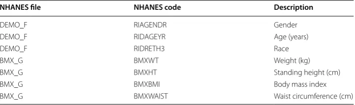
Table 1 shows a selection of demographic variables used. In consulting with medical professionals, it was suggested that these were very common features a doctor would first evaluate when exposed to a new patient and related works previously cited confirm these decisions.
As seen in Table 2 several laboratory results were additionally chosen. Blood pressure and cholesterol have been linked to chronic heart conditions and including such meas-urements will improve our model.
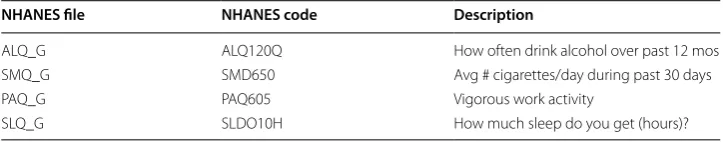
Finally we look at lifestyle choices in Table 3. The WHO has released several techni-cal reports which show the adverse effects of smoking and drinking to long term health. Alcohol is known to adversely affect liver and kidney function while smoking causes many chronic lung and vascular conditions.
Table 1 NHANES variables
NHANES file NHANES code Description
DEMO_F RIAGENDR Gender
DEMO_F RIDAGEYR Age (years)
DEMO_F RIDRETH3 Race
BMX_G BMXWT Weight (kg)
BMX_G BMXHT Standing height (cm)
BMX_G BMXBMI Body mass index
Feature engineering
The foundation of our model creation lies in feature engineering. The NHANES dataset contains many features that are not in an optimal form to be used by machine learning algorithms. Attempting to manually adjust thousands of features would be impractical. Medical experts and literature were consulted to determine which features to include, and only those features were adjusted to a form most usable by most algorithms. This method is known as expert feature selection.
Though a large number of features need adjustment to be understood by machine learning algorithms, a non-trivial number were found to be useful as-is. Feature selec-tion algorithms were applied in an attempt to find features which may have not occurred to domain experts to include. The newly found features were then reviewed before inclu-sion to make sure they were applicable to our problem and not found by coincidence. Additionally, the intersection of features suggested by domain experts and features found algorithmically are analyzed. Algorithmic feature selection which agrees with many of the features found by medical experts would increase confidence in the process.
While it may seem counter-intuitive that such a large expansive survey would create features which are not optimal for machine learning algorithms, many of the features are collected in a form which is most common to the clinical setting. In the clinical setting, results would most often be analyzed by a medical professional, not an algorithm.
In the case of lab results, blood pressure is sampled on four separate occasions. This is not an optimal representation for machine learning as some algorithms assume inde-pendence between features and this is not the case. Multiple lab samples of the same measurement are aggregated into a single mean feature in order to increase learning potential.
Many survey questions are additionally split into multiple features. An example of this is SMQ050Q—“How long since quit smoking cigarettes?” The answer given does not Table 2 Laboratory NHANES variables
NHANES file NHANES code Description
BPX_G BPXSY [1–4] Systolic blood pressure (mmHg)
BPX_G BPXDI [1–4] Diastolic blood pressure (mmHg)
TCHOL_G LBXTC Total cholesterol (mg/dL)
TRYGLI_G LBXTR Triglyceride (mg/dL)
TRYGLI_G LBDLDL LDL cholesterol (mg/dL)
HDL_G LBDHDD Direct HDL cholesterol (mg/dL)
Table 3 Lifestyle NHANES variables
NHANES file NHANES code Description
ALQ_G ALQ120Q How often drink alcohol over past 12 mos
SMQ_G SMD650 Avg # cigarettes/day during past 30 days
PAQ_G PAQ605 Vigorous work activity
contain units and the subsequent question SMQ050U—“Unit of measure” must be con-sulted to calculate a properly scaled number.
Multi-part answers may not contain survey questions applicable to all participants. For example, SMQ020—“Have you smoked at least 100 cigarettes in your life?” Those that answer “no” are not asked follow up questions such as SMD030—“Age that you started smoking cigarettes regularly.” The NHANES survey methodology uses a missing value entry (denoted as a question mark “?” in Weka). In order to assist machine learning algo-rithms differentiate missing values due to non-applicability and missing values due to survey issues, multi-part questions that disqualify future answers are typically converted to a 0 or −1 (depending the context). In the case of SMD030, 0 represents “Have smoked but never on a regular basis” and we convert missing values due to never having smoked to −1 representing “Never smoked.”
NHANES often has a “Refused” and “Don’t Know” choice for survey questions. These are encoded by the CDC as a very large number that could not be mistaken for a valid value. For example, in SMD030, the respondent not knowing the age in which they started smoking is encoded as 999. It should be obvious to a human observer that this is not a valid value. However, many machine learning algorithms do not have built-in outlier detection and such a large value may have undue influence over the final model, reducing performance.
Algorithmic feature selection
For this research, the filter feature selection method is chosen. Filter methods are typi-cally much less computationally intensive than wrapper methods [40]. While embedded methods may yield good results with a low amount of computational complexity, using embedded methods would limit the number of classification algorithms for comparison. The two algorithms chosen for feature selection are gain ratio (GR) and Chi Squared (CS).
The CS test has its history in statistics as a test to determine the independence of two events. GR is a variant of the information gain (IG) algorithm that attempts to penalize attributes which cause a large number of splits. IG tends to prefer splitting on attributes which have many distinct values. In the extreme case, assigning a numeric ID to each instance would cause IG to assign that feature a very high score. However, it should be obvious that this would create a model that is overfit and would not perform well on unseen instances.
Features discovered by GR and CS are ranked by their respective algorithms with regard to ability to predict the outcome variable. The best 100 features are chosen from each result and the intersection of features is used as the final set of algorithmically cho-sen features, as shown in the equation above. SCS represents the best 100 features found
by the GR algorithm and SGR represents the best 100 features by the GR algorithm. Salg represents the resultant set of features to be used in union with expert feature selection.
Salg=SCS
Hybrid feature selection
Once discovered features are reviewed and engineered, a final set of features consist-ing of the union of medical expert feature selection and algorithmic feature selection is created (as shown in the equation below). Sexpert represents the set of features found by
domain expert feature selection and Sresult represents the final set of features to be used
with classification algorithms.
This final set of features is the hybrid feature selection method. Predictive models and wellness scores are created using expert only and hybrid feature selection methods. The resultant predictive models are then compared using a two sample t test in order to test if the hybrid model is superior.
Classification algorithms
The predictive modeling approaches for this research include artificial neural networks, decision trees, simple probabilistic classifiers, and ensembles. The learning task in this research is known as supervised learning. In supervised learning, the goal is to train a model with input variables to predict a desired output variable. The models are then tested with an additional dataset that conforms to the same distribution of variables as the training data to determine the performance.
Multilayer perceptrons
Artificial neural networks (ANN) are a family of machine learning models inspired by the human brain. Nodes are meant to model the biological function of neurons. Each node is assigned a weight that works with activation functions to determine output var-iables. While originally rooted in human biology, modern ANN’s are often developed using statistics and signal processing.
Multilayer perceptrons (MLP) are a type of feed-forward ANN that includes a tech-nique for training known as backpropagation. The purpose of backpropagation is to feed training errors back to the optimization method which uses the information to assist in minimizing the loss function [41]. MLP consists of an input and output layer with one or more hidden layers. This can be represented as a directed acyclic graph (DAG) with each layer being fully connected to the next.
ANN are able to build networks which can model non-linear data with many input values. They are known to build models which can be difficult for humans to interpret. Some algorithms may require a great deal of parameter tuning and retraining as well. ANN may be computationally intensive to train and need additional preprocessing whereby data is centered and scaled.
Radial basis function network
Radial basis function networks are a type of ANN that uses radial basis functions (RBF) as the activation function. RBF networks have the same general architecture as other ANN. The differentiating characteristic of RBF networks is that they are able to learn nonlinear functions, which some ANN cannot. RBF work by calculating the radial
Sresult=Salg
distance from a central point for each instance. This non-linear transformation allows RBF Networks to correctly predict the XOR classification problem of which some ANN are incapable [42].
C4.5
Decision trees are a class of models which use a tree-like graph to walk through a set of decisions which determine an answer. Many algorithms exist for training decision trees, most notably the ID3 algorithm. ID3 uses the concept of entropy to determine which attribute to choose as a decision node. Then a subset is created using that attribute and algorithm is repeated recursively until a stopping point is reached. Various methods for stopping exist. The most popular are predefining a maximum desired tree height or min-imum number of children. C4.5 is a decision tree algorithm is an improvement upon the ID3 decision tree algorithm which uses gain ratio (GR) as the splitting criteria. GR penalizes attributes that have many values and reduces overfitting [43]. The J48 algo-rithm is a Java implementation of C4.5 and is the implementation used in this research.
Decision trees are popular in decision support systems (DSS) because they can be easily visualized and results interpreted by a human. Decision trees do not require that attributes be centered and scaled, nor do they require dummy variables as they can han-dle categorical variables natively. While building a decision tree may be computationally intensive, a completed tree can arrive at a decision quickly. Decision trees also have the ability to discard irrelevant variables. Decision trees do not require a separate missing value strategy, though it is often the case a strategy is chosen in the preprocessing phase.
Decision trees often need pruning rules to keep trees from growing too large and over-fitting the data. Some concepts, such as the XOR, are not modeled easily by decision trees and will often produce a large and complex tree. Decision trees use greedy algo-rithms and may not produce a globally optimum tree [44]. Decision trees are unstable learners. A small change in training data can sometimes have a large effect on the tree. However, when used with ensemble learners, this characteristic can be advantageous [32].
Naïve Bayes
Simple probabilistic classifiers include the Naïve Bayes (NB) classifier. NB is based upon Bayes’ theorem and assumes conditional independence between features. While this may often not be the case with a given dataset, many times NB is still able to classify with good-enough performance [45]. If the NB conditional independence assumption holds, NB is able to converge with fewer data than many other models [46]. NB is popu-lar in real-time (or near real-time) systems as it is both fast to train and fast to classify.
Bayesian network
BN is represented by a DAG which can be visually drawn. This means that the results are often interpretable by a human. BN is known to address the problem of overfitting and handles missing data well. Several variants exist, including Tree Augmented BN (TAN), BN Augmented NB (BAN), and General BN (GBN). BN use the concept of a Markov blanket which acts as embedded feature selection [48].
Support vector machines
Support vector machines (SVM) are a type of classifier which creates a hyperplane that attempts to maximize the margin between classes. SVM is able to map inputs to higher dimensional feature spaces, thereby enabling it to do non-linear classification [49]. This gives SVM additional flexibility linear classifiers do not possess. SVM also have strong statistical theoretical foundations that many other classifiers do not possess and whose model is the global optimum. Additionally SVM is a stable algorithm whose model will not change much with the addition of a small number of instances.
SVM are often difficult to interpret when compared to methods such as decision trees and need additional selection of an appropriate kernel function. The selection of a proper kernel function allows the application of domain knowledge to the dataset, but improper selection can be detrimental to performance. The Java based SMO implemen-tation of SVM is used for this particular research.
Ensemble learning
Ensemble learning is a class of meta-algorithms that uses algorithms in combination with traditional algorithms to solve specific issues such as bias. They offer additional advantages from multiple perspectives. From a statistical point of view, ensembles are able to make use of limited data efficiently [32]. A method known as Bagging is a direct adaptation of the statistical resampling technique known as bootstrapping. Many machine algorithms find local rather than global optima. This may cause them to find a local solution which may not be very good compared to other local optima [32]. Ensem-bles build many models and can often overcome this limitation.
Bagging
Bagging (also known as bootstrap aggregation) is an ensemble learner that attempts to improve the stability of the classifiers and reduce variance. Bagging works well with unstable classifiers such as decision trees [31]. The algorithm works by sampling with replacement, thus creating a number of so-called bags. Each bag contains a sample rep-resentative of the original dataset and the sampling is done with replacement.
Adaboost
Random forest
Random forests (RF) are a type of ensemble learning. RF is part of a family of algorithms known as decision trees. As previously discussed, ID3 is an example of a decision tree algorithm. The advantages of RF is that they are less prone to overfitting than many other decision tree algorithms [50]. RF accomplishes this by averaging multiple decision trees. An advantage of most decision tree algorithms are they can be interpreted visually as a graphical tree structure. However RF loses this feature as many trees are used in the final model. RF works by applying bagging techniques to both instances and features.
RF is less prone to overfitting than a single tree. In practice, RF is known to perform well on many datasets. As with building a single decision tree, RF can be computation-ally complex to build, but quick to classify new data. RF lends itself to parallelization as each tree can be built independently and classify new data independently. Trees built by RF can be much more difficult for a human to interpret than a single decision tree.
Over and under sampling
Algorithms trained from imbalanced data will often time favor the majority class pro-ducing models which may be incapable of predicting the minority class. Early work on this framework revealed the need to explore resampling as several models were unable to predict self-assessment scores of 1 and 5. While many approaches exist for over and under sampling [51], simple over sampling of the minority (scores 1 and 5) by 50 % and under sampling the majority by 30 % (score 3) proved sufficient. Only the data with which models were trained was resampled. Test data remained unmodified as to main-tain the integrity of the research.
Weka and R
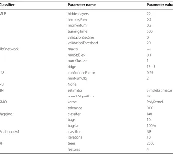
Preprocessing tasks are scripted in the R programming language. R is a direct descend-ant of the S statistical language and has many built-in libraries for data manipulation. Statistical significance tests of resultant AUC data is also programmed in R using the t.test() function. Machine learning models are created using the Weka machine learning toolkit. Weka is written in the Java programming language and has many machine learn-ing algorithms available. Parameters chosen for our models is listed in Table 4. Many of these are suggested by the Weka software as reasonable defaults.
Wellness model
are aggregated using the mean of self-assessment prediction. The resultant models are equally weighted.
where n is the number of classifiers built for dataset D, and Ci is the classification pre-dicted by the ith evaluator. A scaling factor of 20 is applied to scale the wellness score between 1 and 100. This range was arbitrarily chosen as to make the score implications more apparent to a respondent.
Stratified cross validation
In order to use data more efficiently, stratified cross validation is employed. A common method to test the performance of a classification task is to split labelled data into a training set and test set. The training set is used to build the evaluator and test set is used to measure which instances were correctly classified. In many classifications tasks the test data should have the same distribution of outcome variables.
An enhancement to this technique is known as stratified cross validation. The data is split into n stratified partitions and class distribution is preserved (n = 10 for this research). n−1 partitions are combined to form a training set and the remaining
W(D)=
1
n
n
i=1 Ci
·20
Table 4 Weka classification parameters
Classifier Parameter name Parameter value
MLP hiddenLayers 22
learningRate 0.3
momentum 0.2
trainingTime 500
validationSetSize 0
validationThreshold 20
Rbf network maxIts −1
minStdDev 0.1
numClusters 1
ridge 1E−8
J48 confidenceFactor 0.25
minNumObj 2
NB None
BN estimator SimpleEstimator
searchAlgorithm K2
SMO kernel PolyKernel
tolerance 0.001
Bagging classifier J48
bags 10
bagsize 100 %
AdaboostM1 classifier NB
iterations 10
RF trees 2500
partition is used to test the model. Performance metrics are collected and saved. This process is performed iteratively until each partition has had a test data set extracted exactly once. Performance metrics are then aggregated using a method of central ten-dency. In the case of this research the mean AUC is taken as the primary performance metric.
Area under ROC
The NHANES self-assessment response variable is unbalanced as shown in Fig. 3. In cases where the response variable is unbalanced, accuracy is often not an appropriate choice for metrics. Algorithms that favor the majority class will score very high without any regard to their predictive power of the minority classes. The receiver operator char-acteristic (ROC) is often chosen as a performance metric when evaluating imbalanced class distributions. The ROC is a plot of the true positive rate (TPR) and false positive rate (FPR).
Traditional ROC curves are not compatible with multi-class classification tasks. In the case of self-assessment, five possible classifications are possible, thus requiring a slight extension to the traditional definition.
For each classifier, 5 iterations of AUC calculation are performed (corresponding to the 5 possible classification values). The AUC is calculated considering each class value as the positive class and all other classes as the negative class. A weighting mechanism is used as to give each AUC value proportional influence, then the mean of all 5 AUC values is taken to represent the AUC score for that classifier. Repeat this process for all n-folds of stratified cross validation. This is represented by the AUC-Algorithm 1.
An independent two sample t test is performed to compare expert-only variable selec-tion to our hybrid approach. AUC is used as the primary performance metric and is the statistic under comparison. Each fold of our n-fold cross validation is considered a mem-ber of each population therefore giving each population sample size n = 10. The chosen classifiers are then compared for statistical significance using a two sample t test. A value of p ≤ 0.05 considered statistically significant for this research.
Results
Algorithmic feature selection
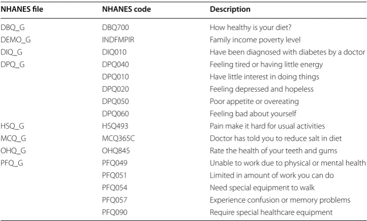
Discovered NHANES variables can be broadly categorized into mental health, oral health, lifestyle limitations, diet, and income level. Acknowledging mental health in the holistic picture of wellness is important. A comprehensive wellness score must not only incorporate physical health but mental health as well. Research has shown there is a cor-relation between chronic physical illness and mental health [52]. Many reasons for this relationship exist. For example, a depressed individual may overeat causing weight gain. Weight gain then (Table 5) may become an additional driver of pre-existing depression. This example is exemplified by the discovered NHANES variable DPQ050—overeating.
Oral health has been shown to be linked with higher occurrence of stroke at an early age [53]. Additionally, there is a correlation between diabetes and periodontal health [54]. Those with poorly controlled diabetes are shown to be 3 times more likely to have periodontal disease than the general population. NHANES diabetes questions appear in both expert selected variables and algorithmically selected variables. The appearance of both oral health and diabetes in variable selection strengthens the consistency of our model.
Income level and diabetes are known to have a strong correlation [56]. Low-income individuals were shown to have poor (Table 6) diets and a strong predictor variable of diabetes. Chronic disease is a major component in wellness. Many inexpensive foods are calorie dense and lead to overeating. Additionally, those faced with food insecurity dur-ing pregnancy and were shown to overconsume calorie dense foods later in life. Many low-income individuals also lack access to medical care and may be unaware of their pre-diabetic conditions.
The table above illustrates the variables found both by algorithmic selection and expert selection. These variables can be categorized into weight, activity level, and recent health. Experts and algorithms both agree that being overweight is a crucial factor in wellness. When creating a wellness plan, addressing weight issues should be considered a priority. Recreational activities are agreed upon as well. It should be noted that work activity was not agreed upon by both experts and algorithms. Recreational activities are typically a life-style choice while activity required by employment many times is not. Those who participate in recreational activity may be consciously choosing a healthy lifestyle. Recent health seems to be an indicator of long-term health and overall wellness as well.
Table 5 Discovered features
NHANES file NHANES code Description
DBQ_G DBQ700 How healthy is your diet?
DEMO_G INDFMPIR Family income poverty level
DIQ_G DIQ010 Have been diagnosed with diabetes by a doctor
DPQ_G DPQ040 Feeling tired or having little energy
DPQ010 Have little interest in doing things
DPQ020 Feeling depressed and hopeless
DPQ050 Poor appetite or overeating
DPQ060 Feeling bad about yourself
HSQ_G HSQ493 Pain make it hard for usual activities
MCQ_G MCQ365C Doctor has told you to reduce salt in diet
OHQ_G OHQ845 Rate the health of your teeth and gums
PFQ_G PFQ049 Unable to work due to physical or mental health
PFQ051 Limited in amount of work you can do
PFQ054 Need special equipment to walk
PFQ057 Experience confusion or memory problems
PFQ090 Require special healthcare equipment
Table 6 Features found by both experts and algorithms
NHANES file NHANES code Description
BMX_G BMXBMI Body mass index
BMX_G BMXWAIST Waist circumference (cm)
HSQ_G HSQ470 No. days in last month health not good
HSQ_G HSQ480 No. days in last month mental health not good
HSQ_G HSQ490 No. days in last month inactive due to health
PAQ_G PAQ650 Vigorous recreational activities
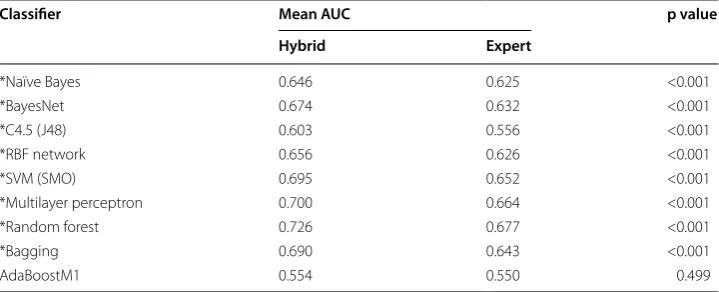
Table 7 shows that in 8 of the 9 classifiers, using a hybrid approach to wellness predic-tion is superior to expert only. Addipredic-tionally, the boxplots in Fig. 4 show the large margin by which many of the classifiers are better. With the large number of variables available in NHANES it would be difficult for a domain expert to adequately explore all variables. However, as previously mentioned, without a large amount of preprocessing and feature engineering, algorithm-only feature selection would generate a lot of noise that may not coincide with known medical research. The results show the practicalities of a hybrid model.
Random forest was shown to be the best overall performer and AdaBoostM1 shown to be the worst. Ensemble methods also improved their base methods with the exception of AdaBoostM1. Each category of classifiers has strengths and weaknesses and resulting models are then aggregated to create the patient’s wellness score.
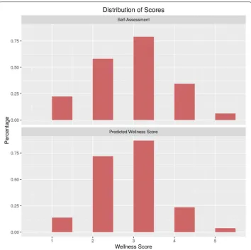
Figure 5 illustrates a comparison of distributions of the wellness score against reported self-assessment. Since the self-assessment ground truth is scaled differently than the final wellness score, the distributions are shown before the wellness score is scaled. The figure represents aggregation of models only, discretized into bins since the aggregated
Table 7 AUC comparison between hybrid and expert models
* Statistical significance, p < 0.05
Classifier Mean AUC p value
Hybrid Expert
*Naïve Bayes 0.646 0.625 <0.001
*BayesNet 0.674 0.632 <0.001
*C4.5 (J48) 0.603 0.556 <0.001
*RBF network 0.656 0.626 <0.001
*SVM (SMO) 0.695 0.652 <0.001
*Multilayer perceptron 0.700 0.664 <0.001
*Random forest 0.726 0.677 <0.001
*Bagging 0.690 0.643 <0.001
AdaBoostM1 0.554 0.550 0.499
wellness score contains real numbers. The score of 3 is not vastly overrepresented and an encouraging outcome. Often times in an unbalanced dataset the majority class may be overrepresented as it is the most frequent case. Table 8 shows the numerical output by which Fig. 5 was built for reference.
Fig. 5 Comparison of self-assessment score distribution and predicted wellness score distribution
Table 8 Distribution of ground truth self-assessment vs wellness model
Score Ground truth Wellness model
1 0.111 0.068
2 0.290 0.359
3 0.395 0.434
4 0.172 0.118
Conclusions
It has been shown that our hybrid approach for generating a wellness score is an improvement upon expert-only methods. With regard to the most important features (weight and activity level) expert and algorithmic models seem to be in agreement. It is our hope that the system is accepted by medical professionals as domain expertise was considered in model creation. Additionally, it is transparent which additional variables were algorithmically chosen and clinical research supports newly discovered variables. It is also our hope that a single numeric score is simple enough for patients to understand and change their lifestyles.
The results additionally indicate that predicting self-assessment is a difficult task. Respondents with similar lab results and vital statistics may self-report differing assess-ments. This can cause algorithms to behave irrationally as there may be cultural biases toward self-assessment. The algorithms may not consider these biases due to latent vari-ables. Ongoing research from our group reports higher AUC’s for non-subjective out-come variables using similar methodology. Self-reporting bias may be further explored in future research in an effort to improve the wellness score.
Borderline predictive cases are also an area to receive further exploration. The dis-tance from the self-assessed value should be taken into account. Mispredicting a score by a single point should be considered to have better performance than a classifier which mispredicts a score by multiple points. When combining models, the AUC should also provide a weight to the final wellness score. Models which have good performance should be rewarded and models with poor performance should be penalized.
The CDC has made several NHANES datasets available, with only minor changes between years. This data can be normalized and combined to form a much larger data-set. Since initial work is now complete finding optimal methods using R and Weka, sys-tems such as Apache Spark and Mahout can be used to quickly process many years of NHANES data in the future.
Finally, integration into current workplace wellness and clinical wellness programs is essential. Consultation of medical staff has been integral to the creation of our score with the intention that acceptance rates among the medical community will be higher than purely algorithmic models. Models whose methods are unclear to staff will remain unused and our selection methods strived to be consistent with their medical training. Authors’ contributions
AA carried out the conception and design of the study, participated in the analysis and interpretation of data, and was involved in drafting and revising the manuscript. CB made substantial contributions to the design of the study, the analy-sis and interpretation of the data, and in drafting and revising the manuscript. RB made substantial contributions to the conception and design of the study, participated in the acquisition, analysis and interpretation of data, and was involved in drafting and revising the manuscript. VR made substantial contributions to the conception of the study, participated in the acquisition, analysis and interpretation of data, and was involved in critically reviewing the manuscript. All authors read and approved the final manuscript.
Author details
1 Department of Computer and Electrical Engineering and Computer Science, College of Engineering, Florida Atlantic University, Boca Raton, FL, USA. 2 Department of IT and Operations Management, College of Business, Florida Atlantic University, Boca Raton, FL, USA. 3 Methodist University Hospital Transplant Institute, Memphis, TN, USA.
Competing interests
The authors declare that they have no competing interests.
References
1. Anspaugh DJ, Hamrick MH, Rosato FD. Wellness: concepts and applications. New York: McGraw-Hill Companies; 2006.
2. Squires D, Anderson C. US Health Care from a global perspective; 2015. http://www.commonwealthfund.org/ publications/issue-briefs/2015/oct/us-health-care-from-a-global-perspective. Accessed 4 Feb 2016.
3. Osborn R, Moulds D, Squires D, Doty MM, Anderson C. International survey of older adults finds shortcomings in access, coordination, and patient-centered care. Health Aff. 2014;33(12):2247–55.
4. Kanter M. Aon Hewitt analysis shows upward trend in US Health Care Cost Increases; 2014. http://ir.aon.com/about- aon/investor-relations/investor-news/news-release-details/2014/Aon-Hewitt-Analysis-Shows-Upward-Trend-in-US-Health-Care-Cost-Increases/default.aspx. Accessed 19 Jan 2016.
5. Centers for Disease Control and Prevention. Worker productivity; 2013. http://www.cdc.gov/workplacehealthpro-motion/businesscase/reasons/productivity.html. Accessed 19 Jan 2016.
6. Toossi M. Labor force projections to 2020: a more slowly growing workforce. Mon Labor Rev; 2012. 7. Coverage E. Patient Protection and Affordable Care Act; 2015. pp. 1–877.
8. Yong PL, Olsen L, Young PL, et al. The healthcare imperative: lowering costs and improving outcomes: workshop series summary. Washington, D.C.: National Academies Press; 2010.
9. Black WC, Gareen IF, Soneji SS, Sicks JD, Keeler EB, Aberle DR, Naeim A, Church TR, Silvestri GR, Gorelick J, Gatsonis C. Cost-effectiveness of CT screening in the National Lung Screening Trial. N Engl J Med. 2014;371(19):1793–802. 10. Paltiel AD, Weinstein MC, Kimmel AD, Seage GR, Losina E, Zhang H, Freedberg KA, Walensky RP, Seage GR III, Losina E,
Zhang H, Freedberg KA, Walensky RP. Expanded screening for HIV in the United States–an analysis of cost-effective-ness. N Engl J Med. 2005;352(6):586–95.
11. Krogsboll LT, Jorgensen KJ, Gronhoj Larsen C, Gotzsche PC. General health checks in adults for reducing morbidity and mortality from disease: cochrane systematic review and meta-analysis. BMJ. 2012;345(203):e7191.
12. Centers for Disease Control and Prevention. NHANES History; 2011. http://www.cdc.gov/nchs/nhanes/history.htm. Accessed 25 May 2015.
13. Centers for Disease Control and Prevention. NHANES 2011–2012 current health status; 2013. http://wwwn.cdc.gov/ Nchs/Nhanes/2011-2012/HSQ_G.htm. Accessed 25 May 2015.
14. Emerman E. Companies are Spending more on corporate wellness programs but employees are leaving millions on the table; 2015. https://www.businessgrouphealth.org/pressroom/pressRelease.cfm?ID=252. Accessed 20 Jan 2016. 15. Hamel L, Firth J, Brodie M. Kaiser health tracking poll; 2014.
http://kff.org/health-reform/poll-finding/kaiser-health-tracking-poll-june-2014/. Accessed 20 Jan 2016.
16. Caloyeras JP, Liu H, Exum E, Broderick M, Mattke S. Managing manifest diseases, but not health risks, saved pepsico money over seven years. Health Aff. 2014;33(1):124–31.
17. Goetzel RZ, Henke RM, Tabrizi M, Pelletier KR, Loeppke R, Ballard DW, Grossmeier J, Anderson DR, Yach D, Kelly RK, et al. Do workplace health promotion (wellness) programs work? J Occup Environ Med. 2014;56(9):927–34. 18. Horwitz JR, Kelly BD, DiNardo JE. Wellness incentives in the workplace: cost savings through cost shifting to
unhealthy workers. Health Aff. 2013;32(3):468–76.
19. IdlerEL Angel RJ. Self-rated health and mortality in the NHANES-I epidemiologic follow-up study. Am J Public Health. 1990;80(4):446–52.
20. Okosun IS, Choi S, Matamoros T, Dever GEA. Obesity is associated with reduced self-rated general health status: evi-dence from a representative sample of White, Black, and Hispanic Americans. Prev Med (Baltim). 2001;32(5):429–36. 21. Behara RS, Agarwal A, Pulumati P, Jain R, Rao V (2014) Predictive modeling for wellness and chronic conditions. 2014
IEEE International conference on bioinformatics and bioengineering. Boca Raton: IEEE. pp. 394–8
22. World Health Organization: WHO. Obesity: preventing and managing the global epidemic. Report of a WHO consul-tation. World Health Organ Tech Rep Ser. 2000;894:1–253.
23. WHO. Global status report on alcohol and health 2014. Glob Status Rep Alcohol. 2014: 1–392.
24. U. S. D. of H. and H. Service. The Health consequences of smoking—50 years of progress A report of the surgeon general. Rockville: U.S. Dep Heal Hum Serv Public Heal Serv Off Surg Gen; 2014.
25. World Health Organisation: WHO. Diet, nutrition and the prevention of chronic diseases. World Health Organ Tech Rep Ser. 2003;916:1–149.
26. Chandrashekar G, Sahin F. A survey on feature selection methods. Comput Electr Eng. 2014;40(1):16–28. 27. Domingos P. A few useful things to know about machine learning. Commun ACM. 2012;55(10):78.
28. Dougherty J, Kohavi R, Sahami M. Supervised and unsupervised discretization of continuous features. Mach Learn Proc Twelfth Int Conf. 1995;54(2):194–202.
29. Learning M, Publishers KA, Zenko B, Giraud-Carrier C, Vilalta R, Brazdil P. Is combining classiers with stacking better than selecting the best one? Knowl Creat Diffus Util. 2004: 255–73.
30. Ting KM, Witten IH. Stacking bagged and dagged models. Proc of ICML’97. 1997: 367–75. 31. Quinlan JR. Bagging, boosting, and C4.5. Proc Thirteen Natl Conf Artif Intell. 1003;5:725–30. 32. Dietterich TG. Ensemble methods in machine learning. Mult Classif Syst. 2000;1857:1–15.
33. Bradley AP. The use of the area under the ROC curve in the evaluation of machine learning algorithms. Pattern Recognit. 1997;30(7):1145–59.
34. Fawcett T. An introduction to ROC analysis. Pattern Recognit Lett. 2006;27(8):861–74.
35. Weiss GM, Provost FJ. Learning when training data are costly: the effect of class distribution on tree induction. J Artif Intell Res. 2003;19:315–54.
36. He H, Garcia EA. Learning from imbalanced data. IEEE Trans Knowl Data Eng. 2009;21(9):1263–84.
37. Van Hulse J, Khoshgoftaar TM, Napolitano A. Experimental perspectives on learning from imbalanced data. Proceed-ings 24th International Conference on Machine Learning. 2007: 935–942.
38. Van Hulse J, Khoshgoftaar TM. Knowledge discovery from imbalanced and noisy data. Data Knowl Eng. 2009;68(12):1513–42.
40. Guyon I, Elisseeff A. An introduction to variable and feature selection. J Mach Learn Res. 2003;3:1157–82.
41. Atlas L, Cole R, Muthusamy Y, Lippman A, Connor J, Park D, El-Sharkawai M, Marks J, et al. A performance comparison of trained multilayer perceptrons and trained classification trees. Proc IEEE. 1990;78(10):1614–9.
42. McGarry KJ, MacIntyre J. Knowledge extraction and insertion from radial basis function networks. IEE Colloq Appl Stat Pattern Recognit. 1999;15:1–6.
43. Quinlan JR. Improved use of continuous attributes in C4.5. J Artif Intell Res. 1996;4:77–90.
44. Bennett KP. Global tree optimization: a non-greedy decision tree algorithm. Comput Sci Stat. 1994;26:156. 45. Lewis DD, N’edellec C, Rouveirol C. Naive (Bayes) at Forty: the independence assumption in information retrieval.
Mach Learn. 1998: 4–15.
46. Rish I, Hellerstein J, Jayram T (2001) An analysis of data characteristics that affect naive Bayes performance. Tec Rep RC21993, IBM Watson.
47. Friedman N, Geiger D, Goldszmit M. Bayesian network classifiers. Mach Learn. 1997;29:131–63.
48. Cheng J, Greiner R. Comparing Bayesian network classifiers. Proceedings of the Fifteenth conference on uncertainty in artificial intelligence; 1999. pp. 1999.
49. Smola A, Schölkopf B. A tutorial on support vector regression. Stat Comput. 2004;14:199–222. 50. Breiman L. Random forests. Mach Learn. 1999;45(5):1–35.
51. Chawla N, Bowyer K. SMOTE: synthetic Minority Over-sampling Technique Nitesh. J Artif Intell Res. 2002;16:321–57. 52. Katon WJ. Clinical and health services relationships between major depression, depressive symptoms, and general
medical illness. Biol Psychiatry. 2003;54(3):216–26.
53. Yoshida M, Murakami T, Yoshimura O, Akagawa Y. The evaluation of oral health in stroke patients. Gerodontology. 2012;29(2):489–93.
54. Preshaw PM. Periodontal disease and diabetes. 2009;37:575–8.
55. Lenze EJ, Rogers JC, Martire LM, Mulsant BH, Rollman BL, Dew MA, Schulz R, Reynolds CF. The association of late-life depression and anxiety with physical disability. Am J Geriatr Psychiatry. 2001;9(2):113–35.