Analysis of hourly road accident counts
using hierarchical clustering and cophenetic
correlation coefficient (CPCC)
Sachin Kumar
1*and Durga Toshniwal
2Background
Road and traffic accidents are one of the major cause of fatality and disability across the world. Road accident can be considered as an event in which a vehicle collides with other vehicle, person or other objects. A road accident not only provides property damage but it may lead to partial or full disability and sometimes can be fatal for human being. Increasing number of road accidents is not a good sign for the transportation safety. The only solution requires the analysis of traffic accident data to identify different causes of road accidents and taking preventive measures.
A variety of research has been done on road accident data from different countries. Various research studies used different techniques to analyze road accident data using statistical techniques and provide fruitful outcomes [1–5]. Different other studies used
Abstract
Road and traffic accidents are an important concern around the world. Road acci-dents not only affects the public health with different level of injury but also results in property damage. Data analysis has the capability to identify the different reasons behind road accidents i.e. traffic characteristics, weather characteristics, road charac-teristics and etc. A variety of research on road accident data analysis has already proves its importance. Some studies focused on identifying factors associated with accident severity while others focused on identifying the associated factors behind accident occurrence. These research analyses used traditional statistical methods as well as data mining methods. Data mining is frequently used method for analyzing road accident data in present research. Trend analysis is another important research area in road accident domain. Trend analysis can assist in identifying the increasing or decreasing accidents rate in different reasons. In this study, we have proposed a method to analyze hourly road accident data using Cophenetic correlation coefficient from Gujarat state in India. The motive of this study is to provide an efficient way to choose the best suit-able distance metric to cluster the series of counts data that provide a better clustering result. The result shows that the proposed method is capable of efficiently group the different districts with similar road accident patterns into single cluster or group which can be further used for trend analysis or similar tasks.
Keywords: Accident analysis, Clustering, Cophenetic correlation coefficient, Data mining
Open Access
© 2016 The Author(s). This article is distributed under the terms of the Creative Commons Attribution 4.0 International License
(http://creativecommons.org/licenses/by/4.0/), which permits unrestricted use, distribution, and reproduction in any medium,
provided you give appropriate credit to the original author(s) and the source, provide a link to the Creative Commons license, and indicate if changes were made.
RESEARCH
*Correspondence: [email protected]
1 Centre for Transportation
data mining techniques to analyze road accident data and also claim that data mining techniques are more advanced and better than traditional statistical techniques [6–10,
21, 22]. Although, both the approaches provided good outcome that certainly useful for traffic accident prediction, [9, 11, 12] reveals that heterogeneity in road accident data exists and should be removed prior to the analysis of road accident data. They also sug-gested that use of suitable clustering techniques prior to the analysis of accident data reduces the heterogeneity from data and can help in revealing hidden information.
Besides all these studies that focused on analyzing road accident data and identifying factors that affects severity of road accident, trend analysis of road accident data can also be useful to understand the nature of road accidents in certain locations. Time series data consists of a set of data points or values which have been measured on a certain fixed interval of time [13]. Time series data is very important and useful to understand the nature of trend in different application such as detecting weather trend and forecast-ing stock market trend over a period of years. This is the motivatforecast-ing factor of this study. In this study, we have distributed 1 year road accident counts into 12 slots. Each slot is representing the total number of road accident that has occurred in 2 h of slots. More specifically, we have divided 24 h in 12 slots with 2 h in each slot and in time series data, slot1 is representing the total number of road accidents occurred in between 00:00 a.m. and 2:00 a.m. in 1 year period. So, we have a total of 60 counts for 5 year duration in our time series data. We have extracted this data for all 26 districts of Gujarat state. In order to analyze this data, we are using hierarchical clustering on all 26 time series data. The problem with hierarchical clustering of time series data is that it is quite difficult and unusual to manually decide the distance metric to be used with clustering algorithm. The wrong selection of distance metric certainly results in bad clusters. Our approach is fairly deal with this problem. Therefore, our method can be applied prior to clustering of data to find the best suitable distance metric for clustering. Hence, prior to clustering, we have used Cophenetic correlation coefficient (CPCC) [14] to compare various dis-tance measures with all seven versions of agglomerative hierarchical clustering. CPCC can be defined as a measure of the correlation between the cophenetic distance of two time series data objects and the original distance matrix. The best distance measure that has the strong CPCC value is chosen for hierarchical clustering on time series data. Clustering on time series data and trend analysis of each cluster shows that all the time series objects in each cluster having similar patterns. Hence, in order to perform trend analysis of time series data from several locations or districts, our approach is suitable to apply prior to start trend analysis of road accidents. The results proves that our approach is capable to put all district that have similar accident patterns in one cluster, that will definitely ease the difficulty in handling road accident time series data of different loca-tions together.
Methods
Time series normalization
time series data to generate better outcomes. We used z-score normalization method to normalize our time series data. Z-score normalization standardized the data points in a range of [0, 1]. Consider a time series T = {T1, T2,…, Tn}, z-score normalization
stand-ardize this time series into a normalize time series NT = {NT1, NT2,…, NTn} such that
where µ(NT) and σ(NT) are the mean and standard deviation respectively of normalized time series NT. The z-score formula for normalizing time series is given by Eq. 1.
Distance measures
There are several distance measure exists [16] such as Euclidean distance, Pearson corre-lation coefficient, Spearman distance and etc. These distances play a very important role in clustering time series data. Some of the distance metric used in this study is briefly discussed as follows:
Euclidean distance
Euclidean distance is one of the popular and classic similarity measure used in various clustering algorithms such as K-means and hierarchical clustering. Euclidean distance can be defined as the distance between two points or vectors in Euclidean norm. Euclid-ean distance between two time series of equal length can be computed using Eq. 2 as follows:
The above equation is used to calculate the distance between two time series of similar length of time sequence n.
City block distance
It is also known as Manhattan distance or absolute value distance. It represents dis-tance between points in a city grid road. The city block disdis-tance between two time series objects can be calculated as
Minkowski distance
The Minkowski distance can be defined as a metric in a normed vector space which can be considered as a generalization of both the Euclidean distance and the Manhat-tan disthe Manhat-tance. The Minkowski disthe Manhat-tance of order p between two points T1 and T2 where, T1 = (T11,T12,…, T1n) and T2 = (T21, T22,…, T2n) can be defined as
µ(NT) ≈ 0 and σ (NT)≈1
(1)
NT= n
i=1
t1−µ(T)
σ(T)
(2) DEuclidean(T1, T2)=
n
j=1
T1j−T2j
2
(3) DCityBlock(T1, T2)=
n
j=1
T1j−T2j
If p ≥ 1, the distance will be the result of Minkowski inequality. If p < 1, it violates the
triangle inequality, hence, for p < 1, it cannot be considered as a metric.
Chebyshev distance
Chebyshev distance is a metric [17] that is defined on a vector space where the distance between two vectors is the greatest of their differences along any coordinate dimension [18]. The Chebyshev distance between two time series objects or points p and q, with standard coordinates pi and qi respectively, is
This distance equals the limit of the Lp metrics
Hence, it is also known as L∞ metric.
Cosine distance
Cosine distance can be defined as a similarity measure between two time series objects that measures the cosine of angle between two time series objects. Cosine similarity is only a judgment of orientation but not magnitude. The cosine of two time series objects can be defined by the following equation:
The cosine distance between two time series objects T1 and T2 can be calculated as
Correlation distance
Correlation distance [19] is a measure of statistical dependence between two time series objects. If the two objects are statistically independent, the correlation between them will be 0. The value for correlation distance ranges from.
[−1, +1] depending upon the negative correlation between two objects or
posi-tive correlation between two objects. The correlation distance between two time series objects T1 and T2 can be calculated as
(4) DMinkowski(T1, T2)=
n
i=1
|T1i−T2i|p 1p
(5) DChebyshev =max(|pi−qi|)
lim
k→∞
n
i=1
|pi−qi|k
1k
a·b= ||a|| ·|b| ·cosθ
(6)
DCosine=1−
T1·T
′
2
T1·T
′
1
·(T2·T2)
′
(7)
DCorrelation =1−
T1−T
′
1
·
T2−T
′
2
′
T1−T
′
1 T1−T
′
1
′ ·
T2−T
′
2
·T2−T
′
2
Spearman distance
This distance based on the Spearman’s correlation coefficient. It is a non-paramet-ric measurement of the statistical dependence between two objects. It describes the strength of the relationship between two objects using a monotonic function. A value of −1 or +1 occurs when both the objects are good monotone function to each other. It can be calculated as
where r1 and r2 are the coordinate-wise rank vectors of T1 and T2 such that ri=(Ti1,Ti2,. . .,Tin).
Cophenetic correlation coefficient (CPCC)
Hierarchical clustering linked together two data points or objects from the original data set at every level until no objects are there to link. The height of the link illustrates the distance between the two clusters which consists of those objects. This height is known as the Cophenetic distance between two objects. The CPCC values close to 1 are consid-ered as good. CPCC can be used to compare the clustering result of same data set using different distance measures or clustering algorithms. In general, CPCC is a measure of how accurately a dendrogram preserves the pair-wise distances between the time series objects.
Suppose we have a time series data to be modeled using a clustering method to pro-duce a dendrogram Ti i.e., a cluster model in which the close data points are clustered together in a hierarchical tree form.
Let dij is the Euclidean distance between the ith and jth time series objects and tij the
dendrogrammatic distance between the two time series objects Ti and Tj. This distance is the height of the node at which these two points are first joined together.
Assuming dij′ be the mean of the dij and t ′
ij be the average of the tij, the cophenetic
correlation coefficient can be denoted as
We will use CPCC to calculate the performance of all distance metric discussed in “Distance measures” section to identify the best distance metric to be used for clustering of hourly road accident count data.
Hierarchical clustering
Hierarchical clustering [20] is a popular unsupervised learning technique that seeks to build a hierarchy of clusters. It is broadly categorized into two categories: agglom-erative and divisive. Agglomagglom-erative clustering follows a bottom up approach, i.e. each data object starts in its own cluster, and further closed objects are merged together and (8)
DSpearman=1−
r1−r
′
1
·
r2−r
′
2
′
r1−r
′
1
·r1−r
′
1
′
r2−r
′
2
·r2−r
′
2
′
(9) CoefficientCPCC=
i<j
dij−d
′
ij
·
tij−t
′ ij i<j
dij−d
′ ij 2 · i<j
tij−t
′
ij
forms new cluster. This process repeats till there are no objects remains to merge. Unlike agglomerative clustering, divisive clustering follows top down approach in which all data objects starts in one cluster and splitting among data objects continues till every data objects belongs to a single cluster. However, agglomerative clustering (running time complexity O(n3)) is computationally efficient than divisive clustering algorithm
(run-ning time complexity O(2n)). Therefore, in this paper, we have used agglomerative
hier-archical clustering algorithm which is given as follows:
Algorithm1: Agglomerative Hierarchical clustering
Input: Hourly time series data set Output: n number of clusters
Procedure:
Assign each time series object into one separate cluster
Calculate the pair wise distances between each clusters using best distance metric
Construct the distance matrix using pair wise distance values Merge the two closest time series objects into one cluster
Calculate the new pair wise distances from new cluster to all clusters Update the distance matrix
Repeat until the distance matrix remains with a single data object
Data set description
The secondary data of hourly count of road accidents for the Gujrat state has been extracted from the data set provided by GVK_EMRI, Gujrat. The data set consists of road accidents count of 26 districts of Gujrat state from January 2010 to December 2014.
Results and discussion
Initially, all time series data of 26 districts are normalized using z-score normalization, i.e., all road accident counts for 26 districts are in such range that there mean is close to 0 and their standard deviation is close to 1.
Distance metric selection
After normalization of the time series data of 26 districts, the next task is to find out the best suitable distance metric to cluster the road accident time series data using hier-archical clustering. Hence, we have calculated the CPCC using all seven versions of agglomerative clustering algorithm with all discussed distance metrics on hourly time series counts of 26 districts of Gujarat. The result of this analysis is shown in Table 1.
Clustering result
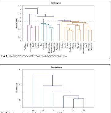
CPCC provides us to perform with the agglomerative hierarchical clustering with aver-age version using Euclidean distance as a distance metric. We then applied agglomerative hierarchical clustering algorithm on our hourly time series data of 26 districts of Gujarat. The dendrogram achieved as a result of clustering process is shown in Fig. 1. Figure 2
Table 1 CPCC analysis for 26 districts of Gujarat for different distance metric
Italic symbol shows the highest CPCC values for average version for AGNES algorithm with Euclidean and Minkowski distance metric
Distance metric Cophenetic correlation coefficient (CPCC)
Single Complete Average Ward Weighted Median Centroid
Euclidean 0.784227 0.791608 0.826298 0.63921 0.760709 0.739566 0.812102 Cityblock 0.795472 0.720603 0.822869 0.617237 0.814186 0.757599 0.800933 Minkowski 0.784227 0.791608 0.826298 0.63921 0.760709 0.739566 0.812102 Chebychev 0.747701 0.621421 0.78132 0.620067 0.756454 0.684826 0.730986 Cosine 0.73324 0.73852 0.779876 0.63823 0.692975 0.70216 0.760326 Correlation 0.733247 0.738506 0.779844 0.638203 0.692964 0.702147 0.760308 Spearman 0.750498 0.528649 0.773012 0.576422 0.725262 0.742434 0.757063
TheDangs
Sura
t
Ah
me
daba
d
Kutch Navsar
i
Valsad Tapi
Narm
ad
a
Daho
d
BanasKanth
a
PanchMahal
s
Sabarkanth
a
Ja
mn
agar
Porbanda
r
Rajkot Anan
d
Khed
a
Gandhinaga
r
Mahesana
Pata
n
Bharuc
h
Vadodara
Surendranaga
r
Am
reli
Bhavnaga
r
Junagadh
0 0.5 1 1.5 2 2.5 3 3.5 4 4.5
Dissimilarit
y
Dendrogram
Fig. 1 Dendrogram achieved after applying hierarchical clustering
C6 C1 C5 C3 C4 C2
2 2.5 3 3.5 4 4.5
Dissimilarity
Dendrogram
illustrates the number of clusters obtained and their linkage using agglomerative hierar-chical clustering. The name of the districts and their cluster id is given in Table 2.
Discussion
The cluster 1 consists of 3 districts, cluster2 consists of 12 districts, cluster3 consists of 6 districts, cluster4 and cluster5 both consists of 2 districts and cluster6 consists of only 1 district of Gujarat state as shown in Table 2. The hourly distribution of the road acci-dents in this district is shown in Figs. 3 and 4. It can be seen from Figs. 3a–c and 4a–c that all districts in each clusters may have different number of accidents but they have similar hourly trend of road accidents. This trend is also following the similar pattern across the years. The more interesting pattern that is found in every cluster is that in every cluster and for every district the highest peak that represents the time slot of 8:00 p.m. to 10:00 p.m. and/or 10:00 p.m. to 12:00 p.m. In this duration the highest numbers of road accidents are reported and these accident counts are increasing every year which is a major concern. The last cluster6 that contains only one district has a slight variation in hourly road accident count for every year but it still preserves the peak at 8:00 p.m. to 10:00 p.m. for road accidents counts.
Hence, our technique of road accident hourly count analysis proves that using our approach we can obtain good quality cluster which consists of districts with similar pat-tern of road accidents in a group or cluster.
Conclusion and future work
This paper presents an approach that makes use of data mining clustering technique to cluster the hourly counts of road accidents of 26 districts of Gujrat for 5 years period that constitutes a time series data. Prior to analysis our approach uses CPCC to find the best distance metric that can be used to cluster our data using agglomerative hierarchi-cal clustering. The Euclidean distance and Minkowski distance (for p = 2) found to be the best suitable distance metric for cluster analysis of 26 time series data. The clustering divides the 26 districts into 6 clusters. In each cluster, the districts with similar accident pattern of road accidents are grouped. The result illustrates that the most dangerous time for road accident is the 8:00 p.m. to 12:00 p.m. in almost all clusters except clus-ter6 that consists of only 1 district which has a slightly varied distribution of accidents across the years. The results simply show that proposed approach is capable to find good
Table 2 Number of clusters and associated districts Cluster Id Name of districts
1 Ahmedabad, Kutch, Surat
2 Amreli, Anand, Bharuch, Bhavnagar, Gandhinagar, Junagadh, Kheda, Mahesana, Patan, Rajkot, Surendranagar, Vadodara
3 BanasKantha, Dahod, Narmada, PanchMahals, Sabarkantha, Tapi
4 Jamnagar, Porbandar
5 Navsari, Valsad
0 500 1000 1500 2000 2500 3000 3500 4000 4500 5000
1 3 5 7 9 11 13 15 17 19 21 23 25 27 29 31 33 35 37 39 41 43 45 47 49 51 53 55 57 59
Surat Kutch Ahmedabad
0 1000 2000 3000 4000 5000 6000 7000 8000 9000
1 3 5 7 9 11 13 15 17 19 21 23 25 27 29 31 33 35 37 39 41 43 45 47 49 51 53 55 57 59
Vadodara Surendranagar Rajkot Patan Mahesana Kheda Junagadh Gandhinagar Bhavnagar Bharuch Anand Amreli
0 500 1000 1500 2000 2500 3000 3500 4000
1 3 5 7 9 11 13 15 17 19 21 23 25 27 29 31 33 35 37 39 41 43 45 47 49 51 53 55 57 59
Tapi Sabarkantha PanchMahals Narmada Dahod BanasKantha a
b
c
Fig. 3 a Hourly distribution of road accidents in cluster 1. b Hourly distribution of road accidents in cluster 2.
0 100 200 300 400 500 600 700 800 a
b
c
1 3 5 7 9 11 13 15 17 19 21 23 25 27 29 31 33 35 37 39 41 43 45 47 49 51 53 55 57 59
Porbandar Jamnagar
0 200 400 600 800 1000 1200 1400
1 3 5 7 9 11 13 15 17 19 21 23 25 27 29 31 33 35 37 39 41 43 45 47 49 51 53 55 57 59
Valsad Navsari
0 10 20 30 40 50 60 70 80 90 100
1 3 5 7 9 11 13 15 17 19 21 23 25 27 29 31 33 35 37 39 41 43 45 47 49 51 53 55 57 59
TheDangs
Fig. 4 a Hourly distribution of road accidents in cluster 4. b Hourly distribution of road accidents in cluster 5.
clusters. The future work will consists of detailed analysis of these clusters with an objec-tive to identify the various locations and factors behind road accidents that occurred during 8:00 p.m. to 10:00 p.m..
Authors’ contributions
DT contributed for the underlying idea and helped drafting the manuscript. DT played a pivotal role guiding and super-vising throughout, from initial conception to the final submission of this manuscript. SK developed and implemented the idea, designed the experiments, analyzed the results and wrote the manuscript. Both authors read and approved the final manuscript.
Author details
1 Centre for Transportation Systems (CTRANS), Indian Institute of Technology Roorkee, Roorkee 247667, Uttarakhand,
India. 2 Computer Science and Engineering Department, Indian Institute of Technology Roorkee, Roorkee 247667,
Uttarakhand, India. Acknowledgements
The authors thankfully acknowledge the GVK-EMRI to provide data for our research. Competing interests
The authors declare that they have no competing interests.
Received: 7 May 2016 Accepted: 16 June 2016
References
1. Miaou SP, Lum H. Modeling vehicle accidents and highway geometric design relationships. Accid Anal Prev. 1993;25(6):689–709.
2. Miaou SP. The Relationship between truck accidents and geometric design of road sections-poisson versus negative binomial regressions. Accid Anal Prev. 1994;26(4):471–82.
3. Ma J, Kockelman K. Crash frequency and severity modeling using clustered data from Washington state. In: IEEE intelligent transportation systems conference. Toronto; 2006.
4. Depaire B, Wets G, Vanhoof K. Traffic accident segmentation by means of latent class clustering. Accid Anal Prev. 2008;40(4):1257–66.
5. Savolainen P, Mannering F, Lord D, Quddus M. The statistical analysis of highway crash-injury severities: a review and assessment of methodological alternatives. Accid Anal Prev. 2011;43(5):1666–76.
6. Chang LY, Chen WC. Data mining of tree based models to analyze freeway accident frequency. J Saf Res. 2005;36(4):365–75.
7. Abellan J, Lopez G, Ona J. Analyis of traffic accident severity using decision rules via decision trees. Expert Syst Appl. 2013;40(15):6047–54.
8. Kashani T, Mohaymany AS, Rajbari A. A data mining approach to identify key factors of traffic injury severity. Promet-Traffic Transp. 2011;23(1):11–7.
9. Kumar S, Toshniwal D. A data mining framework to analyze road accident data. J Big Data. 2015;2(1):1–26. 10. Kumar S, Toshniwal D. A data mining approach to characterize road accident locations. J Mod Transp.
2016;24(1):62–72.
11. Karlaftis M, Tarko A. Heterogeneity considerations in accident modeling. Accid Anal Prev. 1998;30(4):425–33. 12. Oña JD, López G, Mujalli R, Calvo FJ. Analysis of traffic accidents on rural highways using latent class clustering and
Bayesian networks. Accid Anal Prev. 2013;51(2013):1–10.
13. Zhang X, Jun W, Xuecheng Y, Haiying O, Tingjie L. A novel pattern extraction method for time series classification. Optim Eng. 2009;10(2):253–71.
14. Sokal RR, Rohlf FJ. The comparison of dendrograms by objective methods. Taxon. 1962;11:33–40.
15. Ratanamahatana CA, Lin J, Gunopulos D, Keogh E, Vlachos M, Das G. Mining time series data. Data mining and knowledge discovery handbook. Berlin: Springer; 2010. p. 1049–77.
16. Liao TW. Clustering of time series data—a survey. Pattern Recogn. 2005;38(1):1857–74.
17. Cyrus DC. Modern mathematical methods for physicists and engineers. Cambridge: Cambridge University Press; 2000.
18. James MA, Panos MP, Mauricio GC, editors. Handbook of massive data sets. Berlin: Springer; 2002. 19. Gábor JS, Maria LR, Nail KB. Measuring and testing dependence by correlation of distances. Ann. Statist.
2007;35(6):2313–817.
20. Tan PN, Steinbach M, Kumar V. Introduction to data mining. Boston: Pearson Addison-Wesley; 2006.