On sampling theories and discontinuous Dirac systems with eigenparameter in the boundary conditions

R E S E A R C H

Open Access

On sampling theories and discontinuous

Dirac systems with eigenparameter in the

boundary conditions

Mohammed M Tharwat

*_{Correspondence:}

[email protected] Department of Mathematics, Faculty of Science, King Abdulaziz University, Jeddah, Saudi Arabia Department of Mathematics, Faculty of Science, Beni-Suef University, Beni-Suef, Egypt

Abstract

The sampling theory says that a function may be determined by its sampled values at some certain points provided the function satisfies some certain conditions. In this paper we consider a Dirac system which contains an eigenparameter appearing linearly in one condition in addition to an internal point of discontinuity. We closely follow the analysis derived by Annaby and Tharwat (J. Appl. Math. Comput. 2010, doi:10.1007/s12190-010-0404-9) to establish the needed relations for the derivations of the sampling theorems including the construction of Green’s matrix as well as the eigen-vector-function expansion theorem. We derive sampling representations for transforms whose kernels are either solutions or Green’s matrix of the problem. In the special case, when our problem is continuous, the obtained results coincide with the corresponding results in Annaby and Tharwat (J. Appl. Math. Comput. 2010,

doi:10.1007/s12190-010-0404-9).

MSC: 34L16; 94A20; 65L15

Keywords: Dirac systems; transmission conditions; eigenvalue parameter in the boundary conditions; discontinuous boundary value problems

1 Introduction

Sampling theory is one of the most powerful results in signal analysis. It is of great need in signal processing to reconstruct (recover) a signal (function) from its values at a discrete

sequence of points (samples). If this aim is achieved, then an analog (continuous) signal can be transformed into a digital (discrete) one and then it can be recovered by the re-ceiver. If the signal is band-limited, the sampling process can be done via the celebrated Whittaker, Shannon and Kotel’nikov (WSK) sampling theorem [–]. By a band-limited signal with band widthσ,σ> ,i.e., the signal contains no frequencies higher thanσ/π cycles per second (cps), we mean a function in the Paley-Wiener spaceB

σ of entire

func-tions of exponential type at mostσ which areL_{(R)-functions when restricted toR. In}

other words,f(t)∈Bσ if there existsg(·)∈L(–σ,σ) such that,cf.[, ],

f(t) =√ π

σ

–σ

eixtg(x)dx. (.)

Now WSK sampling theorem states [, ]: Iff(t)∈B

σ, then it is completely determined

from its values at the pointstk=kπ/σ,k∈Z, by means of the formula

f(t) =

∞

k=–∞

f(tk)sincσ(t–tk), t∈C, (.)

where

sinct=

sint

t , t= ,

, t= . (.)

The sampling series (.) is absolutely and uniformly convergent on compact subsets ofC. The WSK sampling theorem has been generalized in many different ways. Here we are interested in two extensions. The first is concerned with replacing the equidistant sam-pling points by more general ones, which is very important from the practical point of view. The following theorem which is known in some literature as the Paley-Wiener theo-rem [] gives a sampling theotheo-rem with a more general class of sampling points. Although the theorem in its final form may be attributed to Levinson [] and Kadec [], it could be named after Paley and Wiener who first derived the theorem in a more restrictive form; see [, , ] for more details.

The Paley-Wiener theorem states that if{tk},k∈Z, is a sequence of real numbers such

that

D:=sup

k∈Z

tk–

kπ σ

< π

σ, (.)

andGis the entire function defined by

G(t) := (t–t) ∞

k=

 – t

tk

 – t

t–k

, (.)

then, for any function of the form (.), we have

f(t) =

k∈Z

f(tk)

G(t) G(tk)(t–tk)

, t∈C. (.)

The series (.) converges uniformly on compact subsets ofC.

The WSK sampling theorem is a special case of this theorem because if we choosetk=

kπ/σ= –t–k, then

G(t) =t

∞

k=

 – t

tk

 + t

tk

=t

∞

k=

 –(tσ/π)



k

=sintσ

σ , G

_(t

k) = (–)k.

The sampling series (.) can be regarded as an extension of the classical Lagrange interpo-lation formula toRfor functions of exponential type. Therefore, (.) is called a Lagrange-type interpolation expansion.

such thatK(·,t)∈L_{(I) for allt∈C. Let{t}

k}k∈Zbe a sequence of real numbers such that {K(·,tk)}k∈Zis a complete orthogonal set inL(I). Suppose that

f(t) =

I

K(x,t)g(x)dx,

whereg(·)∈L_{(I). Then}

f(t) =

k∈Z

f(tk) I

K(x,t)K(x,tk)dx

K(·,tk)_L_(I)

. (.)

Series (.) converges uniformly whereverK(·,t)L_(I), as a function oft, is bounded. In

this theorem, sampling representations were given for integral transforms whose kernels are more general thanexp(ixt). Also Kramer’s theorem is a generalization of WSK theo-rem. If we takeK(x,t) =eitx_{,I= [–σ,σ],t}

k=kπ_σ , then (.) is (.).

The relationship between both extensions of WSK sampling theorem has been in-vestigated extensively. Starting from a function theory approach,cf.[], it was proved in [] that if K(x,t), x∈I, t∈C, satisfies some analyticity conditions, then Kramer’s sampling formula (.) turns out to be a Lagrange interpolation one; see also [–]. In another direction, it was shown that Kramer’s expansion (.) could be written as a Lagrange-type interpolation formula if K(·,t) andtk were extracted from ordinary

dif-ferential operators; see the survey [] and the references cited therein. The present work is a continuation of the second direction mentioned above. We prove that in-tegral transforms associated with Dirac systems with an internal point of discontinu-ity can also be reconstructed in a sampling form of Lagrange interpolation type. We would like to mention that works in direction of sampling associated with eigenprob-lems with an eigenparameter in the boundary conditions are few; see,e.g., [–]. Also, papers in sampling with discontinuous eigenproblems are few; see [–]. However, sampling theories associated with Dirac systems which contain eigenparameter in the boundary conditions and have at the same time discontinuity conditions, do not ex-ist as far as we know. Our investigation is be the first in that direction, introducing a good example. To achieve our aim we briefly study the spectral analysis of the prob-lem. Then we derive two sampling theorems using solutions and Green’s matrix respec-tively.

2 The eigenvalue problem

In this section, we define our boundary value problem and state some of its properties. We consider the Dirac system

u_(x) –p(x)u(x) =λu(x),

u_(x) +p(x)u(x) = –λu(x), x∈[–, )∪(, ],

(.)

U(u) :=sinαu(–) –cosαu(–) = , (.)

and transmission conditions

U(u) :=u

––δu

+= , (.)

U(u) :=u

––δu

+= , (.)

whereλ∈C; the real-valued functionsp(·) andp(·) are continuous in [–, ) and (, ]

and have finite limits p(±) :=limx→±p(x) andp(±) :=limx→±p(x); a,a,δ∈R,

α,β∈[,π);δ=  andρ:=acosβ–asinβ> .

In [] the authors discussed problem (.)-(.) but with the conditionsinβu() –

cosβu() =  instead of (.). To formulate a theoretic approach to problem (.)-(.),

we define the Hilbert spaceH=H⊕Cwith an inner product, see [, ],

U(·),V(·)_H:=



–

u(x)v(x)dx+δ 



u(x)v(x)dx+δ



ρzw, (.)

wheredenotes the matrix transpose,

U(x) =

u(x) z

, V(x) =

v(x) w

∈H,

u(x) =

u(x)

u(x)

, v(x) =

v(x)

v(x)

∈H,

ui(·),vi(·)∈L(–, ),i= , ,z,w∈C. For convenience, we put

Ra(u(x))

Rβ(u(x))

:=

au() –au()

sinβu() –cosβu()

. (.)

Equation (.) can be written as

(u) :=Au(x) –P(x)u(x) =λu(x), (.)

where

A=

 

– 

, P(x) =

p(x) 

 p(x)

, u(x) =

u(x)

u(x)

. (.)

For functions u(x), which are defined on [–, )∪(, ] and have finite limitu(±) :=

lim_x→±u(x), byu()(x) andu()(x), we denote the functions

u()(x) =

u(x), x∈[–, ),

u(–_{), x= ,} u()(x) =

u(x), x∈(, ],

u(+_{), x= ,} (.)

which are defined on:= [–, ] and:= [, ], respectively.

In the following lemma, we prove that the eigenvalues of problem (.)-(.) are real.

Proof Assume the contrary that λ is a nonreal eigenvalue of problem (.)-(.). Let

u(x) u(x)

be a corresponding (non-trivial) eigenfunction. By (.), we have

d dx

u(x)u(x) –u(x)u(x)

= (λ–λ)u(x) 

+u(x) 

, x∈[–, )∪(, ].

Integrating the above equation through [–, ] and [, ], we obtain

(λ–λ)



–

u(x)+u(x)

dx

=u

–u

––u

–u

––u(–)u(–) –u(–)u(–)

, (.)

(λ–λ)





_u(x)

+u(x) 

dx

=u()u() –u()u() –

u

+u

+–u

+u

+. (.)

Then from (.), (.) and transmission conditions, we have, respectively,

u(–)u(–) –u(–)u(–) = ,

u()u() –u()u() = –

ρ(λ–λ)|u()|

|a+λsinβ|

and

u

–u

––u

–u

–=δu

+u

+–u

+u

+.

Sinceλ=λ, it follows from the last three equations and (.), (.) that



–

_u(x)

+u(x) 

dx+δ 



_u(x)

+u(x) 

dx= – ρδ

_u ()



|a+λsinβ|

. (.)

This contradicts the conditions _–(|u(x)|+|u(x)|)dx+δ _(|u(x)|+|u(x)|)dx> 

andρ> . Consequently,λmust be real.

LetD(A)⊆Hbe the set of allU(x) =_Ru(x)

β(u(x))

∈Hsuch thatu(i)(·),u(i)(·) are absolutely

continuous oni,i= , , and (u)∈H,sinαu(–) –cosαu(–) = ,ui(–) –δui(+) = ,

i= , . Define the operatorA:D(A) –→Hby

A

u(x)

Rβ(u(x))

=

(u) –Ra(u(x))

,

u(x)

Rβ(u(x))

∈D(A). (.)

Thus, the operatorAis symmetric inH. Indeed, forU(·),V(·)∈D(A),

AU(·),U(·)_H=



–

u(x)v(x)dx+δ 



u(x)v(x)dx

–δ



ρRa

u(x)Rβ

=



–

u_(x) –p(x)u(x)

v(x)dx–



–

u_(x) +p(x)u(x)

v(x)dx

+δ 



u_(x) –p(x)u(x)

v(x)dx

–δ 



u_(x) +p(x)u(x)

v(x)dx

–δ



ρRa

u(x)Rβ

v(x)

= –



–

u(x)

v_(x) +p(x)v(x)

dx+



–

u(x)

v_(x) –p(x)v(x)

dx

–δ 



u(x)

v_(x) +p(x)v(x)

dx

+δ 



u(x)

v_(x) –p(x)v(x)

dx

+u

–v

––u

–v

––u(–)v(–) –u(–)v(–)

+δu()v() –u()v()

–δu

+v

+–u

+v

+

–δ



ρRa

u(x)Rβ

v(x)

= 



u(x) v(x)dx–δ



ρRβ

u(x)Ra

v(x)

=U(·),AV(·)_H.

The operatorA:D(A) –→Hand the eigenvalue problem (.)-(.) have the same eigen-values. Therefore they are equivalent in terms of this aspect.

Lemma . Letλandμbe two different eigenvalues of problem(.)-(.).Then the cor-responding eigenfunctionsu(x)andv(x)of this problem satisfy the following equality:



–

u(x)v(x)dx+δ 



u(x)v(x)dx= –δ



ρRa

u(x)Rβ

v(x). (.)

Proof Equation (.) follows immediately from the orthogonality of the corresponding

eigenelements:

U(x) =

u(x) z

, V(x) =

v(x) w

∈H,

u(x) =

u(x)

u(x)

, v(x) =

v(x)

v(x)

∈H.

Now, we construct a special fundamental system of solutions of equation (.) forλnot being an eigenvalue. Let us consider the next initial value problem:

u_(x) –p(x)u(x) =λu(x), u(x) +p(x)u(x) = –λu(x), x∈(–, ), (.)

By virtue of Theorem . in [], this problem has a unique solutionu=_φφ_(x,λ)(x,λ), which is an entire function ofλ∈Cfor each fixedx∈[–, ]. Similarly, employing the same method as in the proof of Theorem . in [], we see that the problem

u_(x) –p(x)u(x) =λu(x), u(x) +p(x)u(x) = –λu(x), x∈(, ), (.)

u() =a+λcosβ, u() =a+λsinβ (.)

has a unique solutionu=_χχ_(x,λ)(x,λ), which is an entire function of parameterλfor each fixedx∈[, ].

Now the functionsφi(x,λ) andχi(x,λ) are defined in terms ofφi(x,λ) andχi(x,λ),

i= , , respectively, as follows: The initial-value problem,

u_(x) –p(x)u(x) =λu(x), u(x) +p(x)u(x) = –λu(x), x∈(, ), (.)

u() =



δφ(,λ), u() = 

δφ(,λ), (.)

has a unique solutionu=_φφ_(x,λ)(x,λ)for eachλ∈C.

Similarly, the following problem also has a unique solutionu=_χχ(x,λ)_(x,λ):

u_(x) –p(x)u(x) =λu(x), u(x) +p(x)u(x) = –λu(x), x∈(–, ), (.)

u() =δχ(,λ), u() =δχ(,λ). (.)

Let us construct two basic solutions of equation (.) as follows:

φ(·,λ) =

φ(·,λ)

φ(·,λ)

, χ(·,λ) =

χ(·,λ)

χ(·,λ)

,

where

φ(x,λ) =

φ(x,λ), x∈[–, ),

φ(x,λ), x∈(, ],

φ(x,λ) =

φ(x,λ), x∈[–, ),

φ(x,λ), x∈(, ],

(.)

χ(x,λ) =

χ(x,λ), x∈[–, ),

χ(x,λ), x∈(, ],

χ(x,λ) =

χ(x,λ), x∈[–, ),

χ(x,λ), x∈(, ].

(.)

Then

Rβ

χ(x,λ)= –ρ. (.)

By virtue of equations (.) and (.), these solutions satisfy both transmission con-ditions (.) and (.). These functions are entire inλfor allx∈[–, )∪(, ].

LetW(φ,χ)(·,λ) denote the Wronskian ofφ(·,λ) andχ(·,λ) defined in [, p.],i.e.,

W(φ,χ)(·,λ) :=

φ(·,λ) φ(·,λ)

χ(·,λ) χ(·,λ)

It is obvious that the Wronskian

ωi(λ) :=W(φ,χ)(x,λ) =φi(x,λ)χi(x,λ) –φi(x,λ)χi(x,λ), x∈i,i= ,  (.)

are independent ofx∈iand are entire functions. Taking into account (.) and (.),

a short calculation gives

ω(λ) =δω(λ)

for eachλ∈C.

Corollary . The zeros of the functionsω(λ)andω(λ)coincide.

Then we may take into consideration the characteristic functionω(λ) as

ω(λ) :=ω(λ) =δω(λ). (.)

In the following lemma, we show that all eigenvalues of problem (.)-(.) are simple.

Lemma . All eigenvalues of problem(.)-(.)are just zeros of the functionω(λ). More-over,every zero ofω(λ)has multiplicity one.

Proof Since the functionsφ(x,λ) andφ(x,λ) satisfy the boundary condition (.) and

both transmission conditions (.) and (.), to find the eigenvalues of the (.)-(.), we have to insert the functionsφ(x,λ) andφ(x,λ) in the boundary condition (.) and find

the roots of this equation.

By (.) we obtain forλ,μ∈C,λ=μ,

d dx

φ(x,λ)φ(x,μ) –φ(x,μ)φ(x,λ)

= (μ–λ)φ(x,λ)φ(x,μ) +φ(x,λ)φ(x,μ)

.

Integrating the above equation through [–, ] and [, ], and taking into account the initial conditions (.), (.) and (.), we obtain

δφ(,λ)φ(,μ) –φ(,μ)φ(,λ)

= (μ–λ)



–

φ(x,λ)φ(x,μ) +φ(x,λ)φ(x,μ)

dx

+δ 



φ(x,λ)φ(x,μ) +φ(x,λ)φ(x,μ)

dx

. (.)

Dividing both sides of (.) by (λ–μ) and by lettingμ–→λ, we arrive to the relation

δ

φ(,λ)

∂φ(,λ)

∂λ –φ(,λ)

∂φ(,λ)

∂λ

= –



–

φ(x,λ) 

+φ(x,λ) 

dx

+δ 



φ(x,λ) 

+φ(x,λ) 

dx

We show that equation

ω(λ) =W(φ,χ)(,λ) =δ(a+λsinβ)φ(,λ) – (a+λcosβ)φ(,λ)

=  (.)

has only simple roots. Assume the converse,i.e., equation (.) has a double rootλ∗, say. Then the following two equations hold:

a+λ∗sinβ

φ

,λ∗–a+λ∗cosβ

φ

,λ∗= , (.)

sinβφ

,λ∗+a+λ∗sinβ

∂φ(,λ∗)

∂λ

–cosβφ

,λ∗–a+λ∗cosβ

∂φ(,λ∗)

∂λ = . (.)

Sinceρ=  andλ∗is real, then (a+λ∗sinβ)+ (a+λ∗cosβ)= . Leta+λ∗sinβ= .

From (.) and (.),

φ

,λ∗=(a+λ

∗_cosβ)

(a+λ∗sinβ)

φ

,λ∗,

∂φ(,λ∗)

∂λ =

ρφ(,λ∗)

(a+λ∗sinβ)

+(a+λ

∗_cosβ)

(a+λ∗sinβ)

∂φ(,λ∗)

∂λ .

(.)

Combining (.) and (.) withλ=λ∗, we obtain

ρδ(φ(,λ∗))

(a+λ∗sinβ)

= –



–

φ(x,λ) 

+φ(x,λ) 

dx

+δ 



φ(x,λ) 

+φ(x,λ) 

dx

, (.)

contradicting the assumptionρ> . The other case, whena+λ∗cosβ= , can be treated

similarly and the proof is complete.

Let{λn}∞n=–∞denote the sequence of zeros ofω(λ). Then

(x,λn) :=

φ(x,λn)

Rβ(φ(x,λn))

(.)

are the corresponding eigenvectors of the operatorA. SinceAis symmetric, then it is easy to show that the following orthogonality relation holds:

(·,λn),(·,λm)

H=  forn=m. (.)

Here{φ(·,λn)}∞n=–∞is a sequence of eigen-vector-functions of (.)-(.) corresponding to

the eigenvalues{λn}∞n=–∞. We denote by(x,λn) the normalized eigenvectors ofA,i.e.,

(x,λn) :=

(x,λn)

(·,λn)H =

ψ(x,λn)

Rβ(ψ(x,λn))

Sinceχ(·,λ) satisfies (.)-(.), then the eigenvalues are also determinedvia

sinαχ(–,λ) –cosαχ(–,λ) = –ω(λ). (.)

Therefore {χ(·,λn)}∞n=–∞ is another set of eigen-vector-functions which is related by

{φ(·,λn)}∞n=–∞with

χ(x,λn) =cnφ(x,λn), x∈[–, )∪(, ],n∈Z, (.)

wherecn=  are non-zero constants, since all eigenvalues are simple. Since the eigenvalues

are all real, we can take the eigen-vector-functions to be real-valued.

Now we derive the asymptotic formulae of the eigenvalues {λn}∞n=–∞ and the

eigen-vector-functions{φ(·,λn)}∞n=–∞. We transform equations (.), (.), (.) and (.) into

the integral equations, see [], as follows:

φ(x,λ) = cos

λ(x+ ) +α–

x

–

sinλ(x–t)p(t)φ(t,λ)dt

–

x

–

cosλ(x–t)p(t)φ(t,λ)dt, (.)

φ(x,λ) = sin

λ(x+ ) +α+ x

–

cosλ(x–t)p(t)φ(t,λ)dt

–

x

–

sinλ(x–t)p(t)φ(t,λ)dt, (.)

φ(x,λ) = –

 δφ

–,λsin(λx) + δφ

–,λcos(λx) –

x



sinλ(x–t)p(t)φ(t,λ)dt–

x



cosλ(x–t)p(t)φ(t,λ)dt, (.)

φ(x,λ) =

 δφ

–,λsin(λx) +  δφ

–,λcos(λx) +

x



cosλ(x–t)p(t)φ(t,λ)dt

–

x



sinλ(x–t)p(t)φ(t,λ)dt. (.)

For|λ|–→ ∞the following estimates hold uniformly with respect tox,x∈[–, )∪(, ], cf.[, p.],

φ(x,λ) =cos

λ(x+ ) +α+O

 λ

, (.)

φ(x,λ) =sin

λ(x+ ) +α+O

 λ

, (.)

φ(x,λ) = –

 δφ

–,λsin(λx) + δφ

–,λcos(λx) +O

 λ

, (.)

φ(x,λ) =

 δφ

–,λsin(λx) +  δφ

–,λcos(λx) +O

 λ

Now we find an asymptotic formula of the eigenvalues. Since the eigenvalues of the bound-ary value problem (.)-(.) coincide with the roots of the equation

(a+λsinβ)φ(,λ) – (a+λcosβ)φ(,λ) = , (.)

then from the estimates (.), (.) and (.), we get

λsinβ

– δφ

–,λsinλ+ δφ

–,λcosλ

–λcosβ

 δφ

–,λsinλ+ δφ

–,λcosλ

+O() = ,

which can be written as

 δφ

–,λsin(λ–β) +  δφ

–,λcos(λ–β) +O

 λ

= . (.)

Then, from (.) and (.), equation (.) has the form

sin(λ+α–β) +O

 λ

= . (.)

For large|λ|, equation (.) obviously has solutions which, as is not hard to see, have the form

λn+α–β=nπ+δn, n= ,±,±, . . . . (.)

Inserting these values in (.), we find thatsinδn=O(_n),i.e.,δn=O(_n). Thus we obtain

the following asymptotic formula for the eigenvalues:

λn=

nπ+β–α

 +O

 n

, n= ,±,±, . . . . (.)

Using the formulae (.), we obtain the following asymptotic formulae for the eigen-vector-functionsφ(·,λn):

φ(x,λn) =

⎧ ⎪ ⎨ ⎪ ⎩

cos(λn(x+)+α)+O(n) sin(λn(x+)+α)+O(n)

, x∈[–, ), 

δcos(λn(x+)+α)+O( 

n)



δsin(λn(x+)+α)+O( 

n)

, x∈(, ],

(.)

where

φ(x,λn) =

_{φ(x,λn)}

φ(x,λn)

, x∈[–, ), φ(x,λn)

φ(x,λn)

, x∈(, ]. (.)

3 Green’s matrix and expansion theorem

LetF(·) =f(·)

w

resolvent ofA. Indeed, letλbe not an eigenvalue ofAand consider the inhomogeneous problem

(A–λI)U(x) =F(x), U(x) =

u(x) Rβ(u(x))

,

whereIis the identity operator. Since

(A–λI)U(x) =

(u) –Ra(u(x))

–λ

u(x) Rβ(u(x))

=

f(x) w

,

then we have

u_(x) –p(x) +λ

u(x) =f(x),

u_(x) +p(x) +λ

u(x) = –f(x), x∈[–, )∪(, ],

(.)

w= –Ra

u(x)–λRβ

u(x) (.)

and the boundary conditions (.), (.) and (.) withλis not an eigenvalue of problem (.)-(.).

Now, we can represent the general solution of (.) in the following form:

u(x,λ) =

A

φ(x,λ) φ(x,λ)

+B

χ(x,λ) χ(x,λ)

, x∈[–, ), A

φ(x,λ) φ(x,λ)

+B

χ(x,λ) χ(x,λ)

, x∈(, ]. (.)

We applied the standard method of variation of the constants to (.), and thus the func-tionsA(x,λ),B(x,λ) andA(x,λ),B(x,λ) satisfy the linear system of equations

A_(x,λ)φ(x,λ) +B(x,λ)χ(x,λ) =f(x),

A_(x,λ)φ(x,λ) +B(x,λ)χ(x,λ) = –f(x), x∈[–, ),

(.)

and

A_(x,λ)φ(x,λ) +B(x,λ)χ(x,λ) =f(x),

A_(x,λ)φ(x,λ) +B(x,λ)χ(x,λ) = –f(x), x∈(, ].

(.)

Sinceλis not an eigenvalue andω(λ)= , each of the linear system in (.) and (.) has a unique solution which leads to

A(x,λ) =

 ω(λ)



x

χ(ξ,λ)f(ξ)dξ+A,

B(x,λ) =

 ω(λ)

x

–

φ(ξ,λ)f(ξ)dξ+B, x∈[–, ),

(.)

A(x,λ) =

δ

ω(λ) 

x

χ(ξ,λ)f(ξ)dξ+A,

B(x,λ) =

δ ω(λ)

x



φ(ξ,λ)f(ξ)dξ+B,x∈(, ],

whereA,A,BandBare arbitrary constants, and

φ(ξ,λ) =

φ(ξ,λ) φ(ξ,λ)

, ξ∈[–, ), φ(ξ,λ)

φ(ξ,λ)

, ξ∈(, ], χ(ξ,λ) =

χ(ξ,λ) χ(ξ,λ)

, ξ∈[–, ), χ(ξ,λ)

χ(ξ,λ)

, ξ∈(, ].

Substituting equations (.) and (.) into (.), we obtain the solution of (.)

u(x,λ) = ⎧ ⎪ ⎪ ⎪ ⎪ ⎨ ⎪ ⎪ ⎪ ⎪ ⎩

φ(x,λ) ω(λ)



x χ(ξ,λ)f(ξ)dξ

+χ_ω(λ)(x,λ) _–x φ(ξ,λ)f(ξ)dξ+Aφ(x,λ) +Bχ(x,λ), x∈[–, ), δφ(x,λ)

ω(λ) 

xχ(ξ,λ)f(ξ)dξ

+δ_ω(λ)χ(x,λ) _xφ(ξ,λ)f(ξ)dξ+Aφ(x,λ) +Bχ(x,λ), x∈(, ].

(.)

Then from (.), (.) and the transmission conditions (.) and (.), we get

A=

δ ω(λ)





χ(ξ,λ)f(ξ)dξ– wδ



ω(λ), B= ,

A= –

wδ

ω(λ), B=

 ω(λ)



–

φ(ξ,λ)f(ξ)dξ.

Then (.) can be written as

u(x,λ) = –wδ



ω(λ)φ(x,λ) + χ(x,λ)

ω(λ) x

–

a(ξ)φ(ξ,λ)f(ξ)dξ

+φ(x,λ) ω(λ)



x

a(ξ)χ(ξ,λ)f(ξ)dξ, x,ξ∈[–, )∪(, ], (.)

where

a(ξ) =

, ξ∈[–, ),

δ, ξ∈(, ], (.)

which can be written as

u(x,λ) = –wδ



ω(λ)φ(x,λ) + 

–

a(ξ)G(x,ξ,λ)f(ξ)dξ, (.)

where

G(x,ξ,λ) =  ω(λ)

⎧ ⎨ ⎩

χ(x,λ)φ(ξ,λ), –≤ξ≤x≤,x= ,ξ= ,

φ(x,λ)χ(ξ,λ), –≤x≤ξ≤,x= ,ξ= . (.)

Expanding (.) we obtain the concrete form

G(x,ξ,λ) =  ω(λ)

⎧ ⎨ ⎩

φ(ξ,λ)χ(x,λ)φ(ξ,λ)χ(x,λ) φ(ξ,λ)χ(x,λ)φ(ξ,λ)χ(x,λ)

, –≤ξ≤x≤,x= ,ξ= , φ(x,λ)χ(ξ,λ)φ(x,λ)χ(ξ,λ)

φ(x,λ)χ(ξ,λ)φ(x,λ)χ(ξ,λ)

, –≤x≤ξ≤,x= ,ξ= . (.)

only at the eigenvalues. Although Green’s matrix looks as simple as that of Dirac systems, cf.,e.g., [, ], it is rather complicated because of the transmission conditions (see the example at the end of this paper). Therefore

U(x) = (A–λI)–F(x) =

–_ω(λ)wδφ(x,λ) + _– a(ξ)G(x,ξ,λ)f(ξ)dξ Rβ(u(x))

. (.)

Lemma . The operatorAis self-adjoint inH.

Proof SinceAis a symmetric densely defined operator, then it is sufficient to show that the deficiency spaces are the null spaces, and henceA=A∗. Indeed, ifF(x) =f(x)

w

∈H

andλis a non-real number, then taking

U(x) =

u(x) z

=

–_ω(λ)wδφ(x,λ) + _– a(ξ)G(x,ξ,λ)f(ξ)dξ Rβ(u(x))

implies that U∈D(A). Since G(x,ξ,λ) satisfies the conditions (.)-(.), then (A– λI)U(x) =F(x). Now we prove that the inverse of (A–λI) exists. IfAU(x) =λU(x), then

(λ–λ)U(·),U(·)_H=U(·),λU(·)_H–λU(·),U(·)_H

=U(·),AU(·)_H–AU(·),U(·)_H

=  (sinceAis symmetric).

Sinceλ∈/R, we haveλ–λ= . ThusU(·),U(·)H= ,i.e.,U= . ThenR(λ;A) := (A–λI)–, the resolvent operator ofA, exists. Thus

R(λ;A)F= (A–λI)–F=U.

Takeλ=±i. The domains of (A–iI)–_{and (A+iI)}–_{are exactlyH. Consequently, the}

ranges of (A–iI) and (A+iI) are alsoH. Hence the deficiency spaces ofAare

N–i:=N

A∗_{+iI=R(A–iI)}⊥_=H⊥  ={},

Ni:=N

A∗_{–iI=R(A+iI)}⊥_=H⊥  ={}.

HenceAis self-adjoint.

The next theorem is an eigenfunction expansion theorem. The proof is exactly similar to that of Levitan and Sargsjan derived in [, pp.-]; see also [–].

Theorem .

(i) ForU(·)∈H,

U(·)_H=

∞

n=–∞

U(·),n(·)

H



(ii) ForU(·)∈D(A),

U(x) =

∞

n=–∞

U(·),n(·)

Hn(x), (.)

the series being absolutely and uniformly convergent in the first component for on [–, )∪(, ],and absolutely convergent in the second component.

4 The sampling theorems

The first sampling theorem of this section associated with the boundary value problem (.)-(.) is the following theorem.

Theorem . Letf(x) =_f(x)f(x)∈H.Forλ∈C,let

F(λ) = 

–

f(x)φ(x,λ)dx+δ 



f(x)φ(x,λ)dx, (.)

whereφ(·,λ)is the solution defined above.ThenF(λ)is an entire function of exponential type that can be reconstructed from its values at the points{λn}∞n=–∞via the sampling

for-mula

F(λ) =

∞

n=–∞

F(λn)

ω(λ) (λ–λn)ω(λn)

. (.)

The series(.)converges absolutely onCand uniformly on any compact subset ofC,and ω(λ)is the entire function defined in(.).

Proof The relation (.) can be rewritten in the form

F(λ) =F(·),(·,λ)_H=



–

f(x)φ(x,λ)dx+δ 



f(x)φ(x,λ)dx, λ∈C, (.)

where

F(x) =

f(x) 

, (x,λ) =

φ(x,λ) Rβ(φ(x,λ))

∈H.

Since bothF(·) and(·,λ) are inH, then they have the Fourier expansions

F(x) =

∞

n=–∞

f(n) (x,λn) (·,λn)H

, (x,λ) =

∞

n=–∞

(·,λ),(·,λn)

H

(x,λn)

(·,λn)H

, (.)

whereλ∈Candf(n) are the Fourier coefficients

f(n) =F(·),(·,λn)

H=



–

f(x)φ(x,λn)dx+δ





f(x)φ(x,λn)dx. (.)

Applying Parseval’s identity to (.), we obtain

F(λ) =

∞

n=–∞

F(λn)

(·,λ),(·,λn)H (·,λn)H

Now we calculate(·,λ),(·,λn)Hand(·,λn)Hofλ∈C,n∈Z. To prove expansion (.), we need to show that

(·,λ),(·,λn)H (·,λn)H

= ω(λ)

(λ–λn)ω(λ)

, n∈Z,λ∈C. (.)

Indeed, letλ∈Candn∈Zbe fixed. By the definition of the inner product ofH, we have

(·,λ),(·,λn)

H=



–

φ(x,λ)φ(x,λn)dx+δ





φ(x,λ)φ(x,λn)dx

+δ



ρRβ

φ(x,λ)Rβ

φ(x,λn)

. (.)

From Green’s identity, see [, p.], we have

(λn–λ)



–

φ(x,λ)φ(x,λn)dx+δ





φ(x,λ)φ(x,λn)dx

=Wφ–,λ,φ–,λn

–Wφ(–,λ),φ(–,λn)

–δWφ+,λ,φ+,λn

+δWφ(,λ),φ(,λn)

. (.)

Then (.) and the initial conditions (.) imply



–

φ(x,λ)φ(x,λn)dx+δ





φ(x,λ)φ(x,λn)dx=

δ_{W(φ(,λ),φ(,λ} n))

λn–λ

. (.)

From (.), (.) and (.), we have

Wφ(,λ),φ(,λn)

=φ(,λ)φ(,λn) –φ(,λ)φ(,λn)

=c–_n φ(,λ)χ(,λn) –φ(,λ)χ(,λn)

=c–_n (λnsinβ+a)φ(,λ) – (λncosβ+a)φ(,λ)

=c–_n δ–ω(λ) + (λn–λ)Rβ

φ(x,λ). (.)

Also, from (.) we have

δ

ρRβ

φ(x,λ)Rβ

φ(x,λn)

=δ

_c– n

ρ Rβ

φ(x,λ)Rβ

χ(x,λn)

. (.)

Then from (.) and (.) we obtain

δ ρRβ

φ(x,λ)Rβ

φ(x,λn)

= –δc–_nRβ

φ(x,λ). (.)

Substituting from (.), (.) and (.) into (.), we get

(·,λ),(·,λn)

H=c

– n

ω(λ) λn–λ

Lettingλ→λnin (.), since the zeros ofω(λ) are simple, we get

(·,λn),(·,λn)

H=(·,λn)



H= –c

–

nω(λn). (.)

Sinceλ∈Candn∈Zare arbitrary, then (.) and (.) hold for allλ∈Cand alln∈Z. Therefore, from (.) and (.), we get (.). Hence (.) is proved with a pointwise convergence onC. Now we investigate the convergence of (.). First we prove that it is absolutely convergent onC. Using Cauchy-Schwarz’ inequality forλ∈C,

∞

k=–∞

F(λk)

ω(λ) (λ–λk)ω(λk)

≤

_∞

k=–∞

|F(·),(·,λk)H| (·,λk)H

/

×

_∞

k=–∞

|(·,λ),(·,λk)H| (·,λk)H

/

. (.)

SinceF(·),(·,λ)∈H, then the two series on the right-hand side of (.) converge. Thus series (.) converges absolutely onC. As for uniform convergence, letM⊂Cbe compact. Letλ∈MandN> . DefineνN(λ) to be

νN(λ) :=

F(λ) –

N

k=–N

F(λk)

ω(λ) (λ–λk)ω(λk)

. (.)

Using the same method developed above, we get

νN(λ)≤

_N

k=–N

|F(·),(·,λk)H| (·,λk)H

/_N

k=–N

|(·,λ),(·,λk)H| (·,λk)H

/

. (.)

Therefore

νN(λ)≤(·,λk)_H

_N

k=–N

|F(·),(·,λk)H| (·,λk)H

/

. (.)

Since [–, ]×Mis compact, then we can find a positive constantCMsuch that

(·,λ)_H≤CM for allλ∈M. (.)

Then

νN(λ)≤CM

_N

k=–N

|F(·),(·,λk)H| (·,λk)H

/

(.)

uniformly onM. In view of Parseval’s equality,

_N

k=–N

|F(·),(·,λk)H| (·,λk)H

/

ThusνN(λ)→ uniformly onM. Hence (.) converges uniformly onM. ThusF(λ) is an

entire function. From the relation

_F(λ)≤  –

f(x)φ(x,λ)dx+



–

f(x)φ(x,λ)dx

+δ 



f(x)φ(x,λ)dx+δ





f(x)φ(x,λ)dx, λ∈C,

and the fact thatφij(·,λ),i,j= , , are entire functions of exponential type, we conclude

thatF(λ) is of exponential type.

Remark . To see that expansion (.) is a Lagrange-type interpolation, we may replace ω(λ) by the canonical product

ω(λ) = (λ–λ) ∞

n=

 – λ

λn

 – λ

λ–n

. (.)

From Hadamard’s factorization theorem, see [],ω(λ) =h(λ)ω(λ), whereh(λ) is an entire function with no zeros. Thus,

ω(λ) ω(λn)

= h(λ)ω(λ) h(λn)ω(λn)

and (.), (.) remain valid for the functionF(λ)/h(λ). Hence

F(λ) =

∞

n=

F(λn)

h(λ)ω(λ) h(λn)ω(λn)(λ–λn)

. (.)

We may redefine (.) by taking kernel φ_h(λ)(·,λ)=φ(·,λ) to get

F(λ) = F(λ) h(λ) =

∞

n=

F(λn)

ω(λ) (λ–λn)ω(λn)

. (.)

The next theorem is devoted to giving vector-type interpolation sampling expansions associated with problem (.)-(.) for integral transforms whose kernels are defined in terms of Green’s matrix. As we see in (.), Green’s matrixG(x,ξ,λ) of problem (.)-(.) has simple poles at{λk}∞k=–∞. Define the functionG(x,λ) to beG(x,λ) :=ω(λ)G(x,ξ,λ),

whereξ∈[–, )∪(, ] is a fixed point andω(λ) is the function defined in (.) or it is

the canonical product (.).

Theorem . Letf(x) =_f(x)f(x)∈H.LetF(λ) =_F(λ)F(λ)be the vector-valued transform

F(λ) =



–

G(x,λ)f(x)dx+δ 



G(x,λ)f(x)dx. (.)

ThenF(λ)is a valued entire function of exponential type that admits the vector-valued sampling expansion

F(λ) =

∞

n=–∞ F(λn)

ω(λ) (λ–λn)ω(λn)

The vector-valued series(.)converges absolutely onCand uniformly on compact subsets ofC.Here(.)means

F(λ) = ∞

n=–∞

F(λn)

ω(λ) (λ–λn)ω(λn)

, F(λ) =

∞

n=–∞

F(λn)

ω(λ) (λ–λn)ω(λn)

, (.)

where both series converge absolutely onCand uniformly on compact sets ofC.

Proof The integral transform (.) can be written as

F(λ) =G(·,λ),F(·)_H,

F(x) =

f(x) 

, G(x,λ) =

G(x,λ) Rβ(G(x,λ))

∈H.

(.)

Applying Parseval’s identity to (.) with respect to{(·,λn)}∞n=–∞, we obtain

F(λ) =

∞

n=–∞

G(·,λ),(·,λn)

H

F(·),(·,λn)H (·,λn)H

. (.)

Letλ∈Cbe such thatλ=λnforn∈Z. Since each(·,λn) is an eigenvector ofA, then

(A–λI)(x,λn) = (λn–λ)(x,λn).

Thus

(A–λI)–(x,λn) =

 λn–λ

(x,λn). (.)

From (.) and (.) we obtain

–δ

_R

β(φ(x,λn))

ω(λ) φ(ξ,λ) + 

–

a(x)G(x,ξ,λ)φ(x,λn)dx=

 λn–λ

φ(ξ,λn). (.)

Then from (.) and (.) in (.), we get

ρδc– n

ω(λ) φ(ξ,λ) + 

–

a(x)G(x,ξ,λ)φ(x,λn)dx=

 λn–λ

φ(ξ,λn). (.)

Hence equation (.) can be rewritten as

ρδc–_nφ(ξ,λ) +



–

G(x,λ)φ(x,λn)dx+δ





G(x,λ)φ(x,λn)dx

= ω(λ)

λn–λ

φ(ξ,λn). (.)

The definition ofG(·,λ) implies

G(·,λ),(·,λn)

H=



–

G(x,λ)φ(x,λn)dx+δ





G(x,λ)φ(x,λn)dx

+ ρRβ

G(x,λ)Rβ

φ(x,λn)

Moreover, from (.) we have

Rβ

G(x,λ)=φ(ξ,λ)Rβ

χ(x,λ). (.)

Then from (.), (.) and (.) in (.), we obtain

G(·,λ),(·,λn)

H=



–

G(x,λ)φ(x,λn)dx+δ





G(x,λ)φ(x,λn)dx

+ρδc–_nφ(ξ,λ). (.)

Combining (.) and (.), yields

G(·,λ),(·,λn)

H=

ω(λ) λn–λ

φ(ξ,λn). (.)

Taking the limit whenλ–→λnin (.), we get

F(λn) = lim λ→λn

G(·,λ),F(·)_H

= lim

λ→λn

∞

k=–∞

G(·,λ),(·,λk)

H

(·,λk),F(·)H (·,λk)H

. (.)

Making use of (.), we may rewrite (.) as,ξ∈[–, )∪(, ],

F(λn) =

F(λn)

F(λn)

= ⎛ ⎝limλ→λn

∞

k=–∞ ω(λ)

λk–λφ(ξ,λk)

(·,λk),F(·)H (·,λk)H

limλ→λn

∞

k=–∞ ω(λ)

λk–λφ(ξ,λk)

(·,λk),F(·)H (·,λk)H

⎞ ⎠

= ⎛

⎝–ω(λn)φ(ξ,λn)

(·,λn),F(·)H (·,λn)H

–ω(λn)φ(ξ,λn)(·,λ_(·n_,λ),F(·)H

n)_H

⎞

⎠. (.)

The interchange of the limit and summation is justified by the asymptotic behavior of (x,λn) and that ofω(λ). Ifφ(ξ,λn)=  andφ(ξ,λn)= , then (.) gives

F(·),(·,λn)H (·,λn)H

= – F(λn) ω(λn)φ(ξ,λn)

F(·),(·,λn)H (·,λn)H

= – F(λn) ω(λn)φ(ξ,λn)

. (.)

Combining (.), (.) and (.), we get (.) under the assumption thatφ(ξ,λn)= 

andφ(ξ,λn)=  for alln. Ifφi(ξ,λn) = , for somen,i=  or , the same expansions hold

withFi(λn) = . The convergence properties as well as the analytic and growth properties

can be established as in Theorem . above.

Example . Consider the system

u_–p(x)u=λu, u+p(x)u= –λu, x∈[–, )∪(, ], (.)

sinαu() –cosαu() = , (.)

(cosβ+λsinβ)u() + (sinβ–λcosβ)u() =  (.)

and transmission conditions

u

––δu

+= , (.)

u

––δu

+= . (.)

This problem is a special case of problem (.)-(.) whenp(x) =p(x) =p(x) anda=

cosβ,a= –sinβ. Thenρ=  > . For simplicity, we define

P(x) :=

x

–

p(t)dt, P(x) :=

x



p(t)dt, x∈[–, )∪(, ].

In the notations of the above section, the solutionsφ(·,λ) andχ(·,λ) are

φ(x,λ) = ⎧ ⎨ ⎩

cos[ζ(x,λ)]

sin[ζ(x,λ)]

, x∈[–, ), 

δcos[ζ(x,λ)] 

δsin[ζ(x,λ)]

, x∈(, ], (.)

χ(x,λ) =

δ(–sin[ζ(x,λ)]+λcos[ζ(x,λ)]) δ(cos[ζ(x,λ)]+λsin[ζ(x,λ)])

, x∈[–, ), –sin[ζ(x,λ)]+λcos[ζ(x,λ)]

cos[ζ(x,λ)]+λsin[ζ(x,λ)]

, x∈(, ], (.)

where

ζ(x,λ) :=λ(x+ ) +P(x) +α, ζ(x,λ) :=λ(x– ) –P(x) +β.

The eigenvalues are the solutions of the equation

ω(λ) =δ



δ(cosβ+λsinβ)cos

ζ(,λ)

+

δ(sinβ–λcosβ)sin

ζ(,λ)

= ,

which can be rewritten as

cosζ(,λ) –β

–λsinζ(,λ) –β

= . (.)

Green’s function of problem (.)-(.) is given by

G(x,ξ,λ)

= 

× ⎧ ⎪ ⎪ ⎪ ⎪ ⎪ ⎪ ⎪ ⎪ ⎪ ⎪ ⎪ ⎪ ⎪ ⎪ ⎪ ⎪ ⎪ ⎪ ⎪ ⎪ ⎪ ⎪ ⎪ ⎪ ⎪ ⎪ ⎪ ⎪ ⎪ ⎪ ⎨ ⎪ ⎪ ⎪ ⎪ ⎪ ⎪ ⎪ ⎪ ⎪ ⎪ ⎪ ⎪ ⎪ ⎪ ⎪ ⎪ ⎪ ⎪ ⎪ ⎪ ⎪ ⎪ ⎪ ⎪ ⎪ ⎪ ⎪ ⎪ ⎪ ⎪ ⎩

δcos[ζ(ξ,λ)](–sin[ζ(x,λ)]+λcos[ζ(x,λ)])δsin[ζ(ξ,λ)](–sin[ζ(x,λ)]+λcos[ζ(x,λ)]) δcos[ζ(ξ,λ)](cos[ζ(x,λ)]+λsin[ζ(x,λ)]) δsin[ζ(ξ,λ)](cos[ζ(x,λ)]+λsin[ζ(x,λ)])

,

–≤ξ≤x< ,

δcos[ζ(x,λ)](–sin[ζ(ξ,λ)]+λcos[ζ(ξ,λ)])δcos[ζ(x,λ)](cos[ζ(ξ,λ)]+λsin[ζ(ξ,λ)]) δsin[ζ(x,λ)](–sin[ζ(ξ,λ)]+λcos[ζ(ξ,λ)])δsin[ζ(x,λ)](cos[ζ(ξ,λ)]+λsin[ζ(ξ,λ)])

,

–≤x≤ξ< ,

cos[ζ(ξ,λ)](–sin[ζ(x,λ)]+λcos[ζ(x,λ)])sin[ζ(ξ,λ)](–sin[ζ(x,λ)]+λcos[ζ(x,λ)])

cos[ζ(ξ,λ)](cos[ζ(x,λ)]+λsin[ζ(x,λ)]) sin[ζ(ξ,λ)](cos[ζ(x,λ)]+λsin[ζ(x,λ)])

,

–≤ξ< ,  <x≤,

cos[ζ(x,λ)](–sin[ζ(ξ,λ)]+λcos[ζ(ξ,λ)])cos[ζ(x,λ)](cos[ζ(ξ,λ)]+λsin[ζ(ξ,λ)])

sin[ζ(x,λ)](–sin[ζ(ξ,λ)]+λcos[ζ(ξ,λ)])sin[ζ(x,λ)](cos[ζ(ξ,λ)]+λsin[ζ(ξ,λ)])

,

–≤x< ,  <ξ≤, 

δcos[ζ(ξ,λ)](–sin[ζ(x,λ)]+λcos[ζ(x,λ)])δsin[ζ(ξ,λ)](–sin[ζ(x,λ)]+λcos[ζ(x,λ)]) 

δcos[ζ(ξ,λ)](cos[ζ(x,λ)]+λsin[ζ(x,λ)]) δsin[ζ(ξ,λ)](cos[ζ(x,λ)]+λsin[ζ(x,λ)])

,

 <ξ≤x≤, 

δcos[ζ(x,λ)](–sin[ζ(ξ,λ)]+λcos[ζ(ξ,λ)])δcos[ζ(x,λ)](cos[ζ(ξ,λ)]+λsin[ζ(ξ,λ)]) 

δsin[ζ(x,λ)](–sin[ζ(ξ,λ)]+λcos[ζ(ξ,λ)]) δsin[ζ(x,λ)](cos[ζ(ξ,λ)]+λsin[ζ(ξ,λ)])

,

 <x≤ξ≤.

(.)

By Theorem ., the transform

F(λ) = 

–

f(x)cos

ζ(x,λ)

+f(x)sin

ζ(x,λ)

dx

+δ 



f(x)cos

ζ(x,λ)

+f(x)sin

ζ(x,λ)

dx (.)

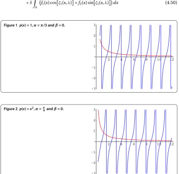
Figure 1 p(x) = 1,α=π/3 andβ= 0.

Figure 2 p(x) =x2_,α=π