E
SSAYS ON THE ECONOMIC IMPLICATIONS OF CLIMATE
CHANGE UNCERTAINTIES
Louise Kessler
September 2017
____________________________________________
A thesis submitted to the Department of Geography & Environment of the London School of Economics and Political Science for the degree of Doctor of Philosophy in
1
DECLARATION
I certify that the thesis I have presented for examination for the MPhil/PhD degree of the London School of Economics and Political Science is solely my own work other than where I have clearly indicated that it is the work of others (in which case the extent of any work carried out jointly by me and any other person is clearly identified in it).
The copyright of this thesis rests with the author. Quotation from it is permitted, provided that full acknowledgement is made. This thesis may not be reproduced without my prior written consent.
I warrant that this authorisation does not, to the best of my belief, infringe the rights of any third party.
I declare that my thesis consists of 57,205 words.
STATEMENT OF CONJOINT WORK
I confirm that Chapter 2 was co-authored with Professor Simon Dietz at the London School of Economics and Political Science and Professor Christian Gollier at the Toulouse School of Economics, and I contributed 33% of this work.
I confirm that Chapter 5 was co-authored with Professor Simon Dietz and Dr. Alex Bowen of the Grantham Research Institute at LSE, and I contributed 75% of this work.
STATEMENT OF PRIOR PUBLICATION
A version of Chapter 2 is publicly available as “The climate beta”, Journal of Environmental Economics and Management, 2017.
2
ABSTRACT
This thesis investigates the economic implications of climate change uncertainties. It seeks to contribute to the existing literature by exploring various aspects of how uncertainty can and should be integrated in economic assessments of climate impacts and what this entails for policy-making.
For several reasons, including analytical tractability and the difficulties of accommodating uncertainty in individual and social decision-making, the full scale of climate change uncertainties is often artificially reduced in economic assessments of climate change, e.g. through the use of best estimates, averages or mid-point scenarios. However, the impacts of future climate change on humankind are highly uncertain and require full investigation. The approach taken in this thesis has therefore been to ask new questions related to the economic implications of climate change uncertainties and to address each problem using innovative methods, which allow a more accurate characterization of the uncertainties at stake and of their potential interactions.
3
ACKNOWLEDGMENTS
I thought that writing acknowledgments would be the easiest part of my PhD but it turns out that it is no easy feat. I would like to mention everyone who accompanied me on this intellectual journey and who provided logistical or emotional support, but I am unfortunately restricted by word count. To all those not mentioned explicitly here, please be assured that I will thank you in person.
First of all, I would like to thank my supervisor Simon Dietz for his invaluable guidance, feedback, and co-authorship, and for making my doctoral pursuit enlightening, challenging and overall hugely enjoyable. I also express gratitude to Dave Stainforth, for his guidance about what should and should not be done with climate models. I am also grateful to Christian Gollier and Alex Bowen, for their collaboration on Chapters 2 and 4 respectively.
I also acknowledge the Economic and Social Research Council who sponsored my doctoral studentship, and the Grantham Research Institute on Climate Change and the Environment, for providing such a supportive and pleasant work environment, with highly stimulating seminars, regular drinks and the occasional piece of cake. I am well aware of how the concentration of expertise and knowledge in the field of climate change makes the Grantham Institute a unique place to work, to exchange ideas and to do engaging research – I hope I kept the standards up.
I also give my sincerest thanks to mentors who supported the twists and turns of my career, and especially Jean-Christophe Bureau, Mathieu Glachant, Vincent Martinet, Eloick Peyrache and Pierre Ducret. Thank you also to Antoine Dechezlepretre who told me casually about the Grantham doctoral studentships on a skype call back in 2013.
4
Table of Contents
CHAPTER 1: UNCERTAINTY IN CLIMATE CHANGE ECONOMICS ... 7
1. Introduction... 7
2. A survey of uncertainties about the drivers of climate change ... 9
i. Uncertainties pertaining to socioeconomic drivers of climate change ... 9
ii. Uncertainties pertaining to the climate system ... 10
3. A survey of uncertainties about the impacts of climate change ... 13
iii. Uncertainties pertaining to the physical effects of climate change ... 13
iv. Uncertainties pertaining to the socioeconomic impacts of climate change ... 15
4. What are the methods that have been used by economists to estimate the impacts of climate change? 16 5. The role of Integrated Assessment Models as policy tools ... 19
i. Two crucial features of IAMs: the damage function and the discount rate ... 20
ii. Limitations of Integrated Assessment Models ... 23
iii. Alternative approaches to IAMs... 24
6. Dissertation outline ... 26
CHAPTER 2: THE CLIMATE BETA ... 33
1. Introduction... 33
2. The CCAPM beta ... 36
3. A simple analytical model of the climate beta ... 38
4. Estimating beta with DICE ... 44
7. Results and discussion ... 49
8. Conclusion and policy implications ... 53
CHAPTER 3: ESTIMATING THE ECONOMIC IMPACT OF THE PERMAFROST CARBON FEEDBACK ... 61
1. Introduction... 61
2. What is the permafrost carbon feedback? ... 63
5
i. How are climate feedbacks usually characterized? ... 64
ii. Proposed approach – A two-phase model ... 65
iii. Phase 1 – Permafrost thaw ... 65
iv. Phase 2: Carbon decomposition and release as CO2 or CH4 ... 68
v. Integrating our PCF module in DICE-2013R ... 70
4. Results and discussion ... 71
i. Physical impacts of the permafrost carbon feedback ... 72
ii. Economic impacts of the permafrost carbon feedback ... 73
5. Conclusion and policy implications ... 78
CHAPTER 4: WHAT ARE THE IMPACTS OF DROUGHTS ON ECONOMIC GROWTH? EVIDENCE FROM U.S. STATES ... 93
1. Introduction... 93
2. Literature review ... 96
i. On the channels through which droughts affect the economy ... 96
ii. On the economic impacts of droughts ... 97
iii. On the compound impacts of droughts and high temperature events ... 99
3. Contribution of this paper ... 100
4. Methodology ... 100
i. Setting ... 100
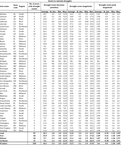
ii. Data ... 102
iii. Scale of the analysis ... 112
iv. Econometric approach ... 113
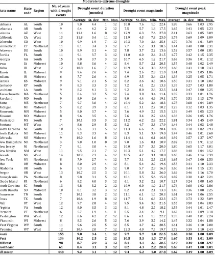
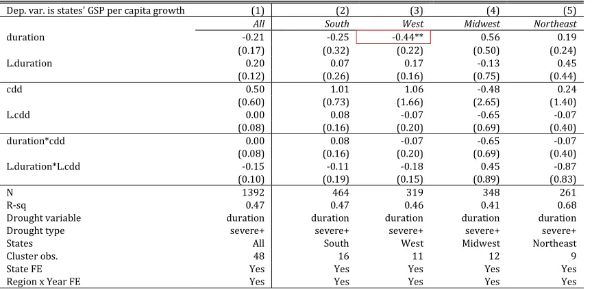
5. Results and discussion ... 113
6. Conclusion and policy implications ... 122
CHAPTER 5: CLIMATE SHOCKS, INFLATION AND MONETARY POLICY: THE GLOBAL EXPERIENCE SINCE 1950 ... 152
1. Introduction... 152
2. Methodology ... 156
i. Data ... 156
ii. Scatter plots ... 160
iii. Econometric approach ... 164
3. Results and discussion ... 165
6
ii. The effects of temperature and precipitation on the annual policy interest rate... 171
iii. Robustness checks ... 177
iv. Discussion of results ... 180
4. Conclusion and policy recommendations ... 182
CHAPTER 6: CONCLUDING THOUGHTS ... 200
1. Insights from previous chapters ... 200
7
Chapter 1:
Uncertainty in climate change economics
“We need not only a new generation of models, but also a broader and wiser set of perspectives on how to use the models that we have, and that we may have, to examine, discuss and propose policies.”
Pr. Nicholas Stern (Stern, 2013)
“Seek simplicity but distrust it.”
Alfred North Whitehead et al. (Whitehead, Griffin, & Sherburne, 1929)
1. Introduction
The emergence of the field of climate change economics can be linked to the fact that, as soon as the scientific community reached a consensus on the anthropogenic origin of climate change, economists have wanted to know two things about climate change: 1) how big will the impacts be? 2) What is their value and how much should we be willing to pay to avoid them? Thanks to the complexity of the task, this research field has flourished: indeed, any attempt at providing a well-informed answer to this question very quickly brings up the following hard fact: that the nature and the scale of the uncertainties pervading every aspect of climate change forestall the possibility of a clear and simple answer.
8
This learning process led me to the overarching question of this PhD: “What are the economic implications of climate change uncertainties?” But given the immensity of the task, the four papers that comprise this PhD are merely small pieces of a big puzzle. The approach I have taken in this thesis has been to find original research questions related to the implications of climate change uncertainties for assessments of the future impacts of climate change, to use innovative ways to address each problem, and to discuss their implications for policy-making.
I have also strived to ensure that these papers reflect the findings of my four-year journey in the deeper recesses of climate change uncertainties. The first one is that the exploration of the implications of climate change uncertainties cannot be done without fully engaging with the multidisciplinarity of the topic. For that reason, I tried to make sure that each of these four papers would put in practice a multidisciplinary approach, which is why I made incursions into the fields of climate models, weather models, biophysics, geology, statistics, and micro- and macro-economics. Rather than a dispersion, I see it as a reflection of the multifacetedness of the issue.
The second one is that, more than the impact of specific uncertainties, what matters ultimately seems to be the impact of combinations of uncertainties. In each paper I have tried to consider multiple uncertainties together and to understand the extent to which the interactions between multiple uncertainties drive outcomes. For instance, Chapter 2 explores the mechanisms through which the interplay of economic and climatic uncertainties drives our results on the “climate beta”.
The third one has been that we need not only to improve the tools that already exist to represent and assess these uncertainties, but also to consider them with fresh eyes and new perspectives – this has been formulated better by Stern (Stern, 2013). Moreover, I have tried to characterize and represent climate uncertainties in ways which make them more tractable, without being unduly restrictive – this has been one of the major concerns for Chapter 3, in which I tried to add a highly uncertain feedback to an existing Integrated Assessment Model. Also, I am well aware of the fact that, given our current level of knowledge, improvements in our understanding of climate processes are likely to increase the range of uncertainties rather than reduce it.
9
2. A survey of uncertainties about the drivers of climate change
i. Uncertainties pertaining to socioeconomic drivers of climate change
The wide uncertainty about the level and timing of future anthropogenic greenhouse gas (GHG) emissions pertains to the fact that these are the product of complex dynamic systems and require projections of demographic development, economic activity, lifestyle, energy use, land use patterns, technology and climate policy (IPCC, 2013; Nakicenovic et al., 2000).
Given the considerable range of factors that influence future emissions paths, a schematic approach based on the Kaya identity (Field & Raupach, 2004) is often used (Nakicenovic et al., 2000): indeed, in this equation, the global carbon dioxide (CO2) emissions flux from fossil fuel combustion is decomposed into four driving forces:
Equation 1.1
𝐹 = 𝑃 ∗ 𝐺 𝑃 ∗
𝐸 𝐺 ∗
𝐹 𝐸
Where:
F is the global CO2 emissions flux from fossil fuel combustion; P is global population;
G is world gross domestic product (GDP); E is global primary energy consumption.
Hence CO2e emissions can be expressed as the product of global population, world per-capita GDP, world energy intensity and the carbon intensity of energy. Thus, the uncertainty about the level of future GHG emissions can be decomposed into the uncertainty about each of these four components.
The uncertainty about world population, which is the first component of the Kaya identity, is non-negligible: according to the United Nations, the upward trend in population size is expected to continue, and the 95% confidence interval of the world’s population by 2100 currently stands at 9.6 to 13.2 billion (United Nations, 2017). The uncertainty about future population growth at the global level stems from the uncertainty about the future levels of fertility and mortality.
10
economy has already benefited from the Internet and web revolution (Gordon, 2015). The second one assumes that the digital revolution will lead to a third technology shock, which will provide similar TFP gains to those that were provided by electricity during the second industrial revolution. According to Cette et al. (2017), the secular stagnation scenario would mean that the yearly rate of TFP growth in the United States over the period 2015-2100 would be around 0.6%, whereas in the technology shock scenario, TFP growth could reach 1.4% per year. These scenarios are useful in that they provide us with an order of magnitude on plausible paths of future TFP growth but should not hide the fact that the long-run average of TFP growth belongs to the realm of deep uncertainties.
The uncertainty about world energy intensity, which is the third component of the Kaya identity, refers to the future levels of energy consumption per dollar of GDP. The scale of the decoupling between energy consumption and economic growth is likely to be driven by two factors. The first one concerns structural changes such as the growing share of the service sector, the replacement of energy-intensive by energy-extensive industries and the dematerialization of the economy. The second one relates to the level of energy-saving technical progress that is achieved. The uncertainty about these factors is further amplified by the fact that they will be highly dependent on regulatory frameworks, research and development policies and societal changes.
Finally, the uncertainty about the carbon intensity of energy, which is the fourth component of the Kaya identity, will depend on the fuel mix of the world economy, which is likely to be driven by two major factors. The first one is technological progress, which could make renewable energy cost-competitive with fossil fuels. This could have considerable implications for CO2 emissions from the power and transportation sectors. The second important one relates to the energy and climate policies which will be put in place over the coming decades. For instance, mitigation policies range from a business-as-usual scenario, which assumes that no major changes in policies will take place, to more aggressive mitigation scenarios, such as those consistent with the 1.5°C target, and which imply achieving net negative CO2 emissions after 2050 (Rogelj et al., 2015).
The uncertainty about the socioeconomic drivers of climate change has been condensed into four scenarios of human activity called the Representative Concentration Pathways (RCPs) (R. H. Moss et al., 2010), which describe four different 21st century pathways of GHG emissions and atmospheric concentrations, air pollutant emissions, land use changes and climate policy. They include one stringent mitigation scenario (RCP2.6), two stabilization scenarios (RCP4.5 and RCP6.0) and one scenario with very high greenhouse gas emissions (RCP8.5). The uncertainty about the level of future GHG emissions appears clearly in the very wide range of cumulative CO2 emissions for the 2012 to 2100 period in each of the four RCP scenarios: these range from 140 to 410 GtC for RCP2.6, 595 to 1,005 GtC to RCP4.5, 840 to 1,250 GtC for RCP6.0 and 1,415 to 1,910 GtC for RCP8.5 (IPCC, 2013).
ii. Uncertainties pertaining to the climate system
11
Since Arrhenius (1896), we have known the basic physics underlying the greenhouse effect, through which greenhouse gases like carbon dioxide (CO2), methane (CH4) and nitrous oxide (NO2) trap solar radiation into the atmosphere, thus making the Earth warmer. What we do not know are the complex processes of the Earth’s climate, which will determine the timing and the scale of the response of the planet to anthropogenic emissions, which is why our projections of future climate change are so imprecise. The uncertainty about the physical drivers of climate change can be segmented into four components: the carbon cycle, the equilibrium climate sensitivity, feedbacks, and potential nonlinearities including tipping points and threshold effects.
The first major uncertainty regarding the physical drivers of climate change is the carbon cycle, i.e. what happens to carbon once it is emitted into the atmosphere. Indeed, the greenhouse effect is based on the concentration of greenhouse gases into the atmosphere, and since these GHGs come from emissions, we need to know how these GHG emissions accumulate in the atmosphere. Oceans play a vital role in the carbon cycle through their uptake of CO2 from the atmosphere and understanding these ocean processes is thus crucial. According to the IPCC, the oceans have de facto absorbed about 30% of the emitted anthropogenic CO2, but there are huge uncertainties about the ocean’s absorptive capacity and whether we should expect it to decrease as oceans undergo acidification and warming (IPCC, 2013). Similarly, carbon residence time is recognized as an important source of model uncertainty (Friend et al., 2014; Yizhao et al., 2015).
The second major uncertainty lies in the relationship between the stock of GHGs in the atmosphere and the expected change in global mean temperature, which has been embodied in the concept of equilibrium climate sensitivity (ECS), defined as the change in global mean surface temperature at equilibrium that is caused by a doubling of the atmospheric CO2 concentration. The ECS is the result of a combination of various positive feedbacks, including the water vapour/lapse rate and the albedo and cloud feedbacks and is generally estimated from Atmosphere-Ocean General Circulation Models. The increasing complexity of our representations of these feedbacks as well as the use of enlarged model ensembles explain why the equilibrium climate sensitivity is one of the components of the climate system for which uncertainty widens as knowledge increases: indeed, whereas the IPCC’s Fourth Assessment Report mentioned that the ECS was likely in the range of 2.0°C to 4.5°C with a best estimate of 3°C (IPCC, 2007), the IPCC’s Fifth Assessment Report stated that the ECS was likely in the range 1.5°C to 4.5°C (IPCC, 2013). Given the reliance of humans and ecosystems on stable temperatures, the discussion on whether or not there is a non-negligible probability that the ECS is around 4.5°C or higher has long expanded outside the field of climate science and has spurred numerous discussions on the implications of “fat tails”1 for decision-making (Calel, Stainforth, & Dietz, 2015; Pindyck, 2013; Weitzman, 2011). These “fat tails” are a direct consequence of the high uncertainty about the feedbacks underlying the ECS and explain why this parameter may well be one of those “known unknowables”.
In many respects, feedback processes are a fundamental component of the uncertainty about future climate change. First, as we have seen above, short-scale feedback processes such as the cloud, albedo and aerosol feedbacks are crucial components of the ECS, i.e., the response of the climate system to an increase in atmospheric CO2 concentration. Moreover, climate change will induce changes in the water, carbon and other biogeochemical cycles, which might trigger,
1 “Fat tails” have been used to refer to the difference in upper tail behaviour between the fat-tailed Pareto distribution
12
reinforce, or overturn feedbacks. These feedbacks can be positive (when they accelerate climate change), or negative (when they dampen climate change). One example of a positive feedback triggered by climate change relates to ocean warming; not only have oceans absorbed a significant share of the CO2 emitted into the atmosphere historically, they have also absorbed part of the radiative imbalance of the climate system, and as a result, have become warmer2. Unfortunately, the solubility of CO2 in seawater decreases as oceans become warmer, which means that as oceans warm, they are less able to remove CO2 from the atmosphere. In this case, climate change triggers a new positive feedback. Other examples of positive feedbacks triggered by climate change include heat-induced releases of sequestered carbon, e.g. from permafrost or offshore methane clathrates. Another reason why feedbacks are a major cause of uncertainty pertains to the fact that positive feedbacks compound each other, meaning that the total effect of two positive feedbacks is larger than the sum of the effects of the individual feedbacks (Roe & Baker, 2007). There is also considerable uncertainty on potential negative feedbacks, such as a cooling effect from CO2-induced increases in vegetation density (Jiang et al., 2012). Finally, it should be emphasized that, despite the advances in our understanding of the climate system, we have an idea of the biophysical processes underlying some feedback loops, but we know close to nothing as to their potential compound strength and the ways in which they might interact with each other – it is also very possible that there are other feedbacks that could be triggered by climate change that we know nothing about. This explains why the IPCC has made clear in its latest report that the Earth system sensitivity over millennial time scales would include long-term feedbacks and would therefore likely be significantly higher than the ECS (IPCC, 2013).
Feedbacks introduce nonlinearities in the response of the climate system, which can then lead to ‘tipping points’, i.e. switches to qualitatively different states (Lenton, 2011). For example, the continued warming of the oceans could lead to a weakening of the Atlantic Meridional Overturning Circulation (AMOC) to a point where it collapses suddenly. The possibility of a collapse of the AMOC happening by 2100 has been estimated as very unlikely by the IPCC but has not been excluded for longer time horizons (IPCC, 2013). Other examples of potential tipping points which could be triggered by human-induced climate change include the irreversible melting of the Greenland and West Antarctic ice sheets, disruptions of the West African monsoon and diebacks of the Amazon and boreal forests (Huntingford et al., 2008; IPCC, 2013).
Due to the deep uncertainty3 that characterizes them, feedbacks and tipping points have so far received little attention in assessments of climate change impacts. We know that these processes could be triggered by climate change, but we have no idea of their potential strength or the time horizon over which they could happen – for that reason, they have been mostly (though not entirely) ignored by climate change economists. We will see further the ways in which these deep uncertainties have been treated in the economics literature, but I argue that this deep uncertainty should be fully acknowledged, brought to the fore, and made an integral part of the policy-making process. Finally, these uncertainties about the physical drivers of climate change contribute to the significant uncertainty regarding the link between temperature targets (e.g. 2°C) and the corresponding carbon budget (IPCC, 2013).
2 According to the IPCC, ocean warming dominates the increase in energy stored in the climate system, accounting for
more than 90% of the energy accumulated between 1971 and 2010 (IPCC, 2013)
3 Deep uncertainty has been defined by Hallegatte et al. (2012) as “a situation in which analysts do not know or cannot
13
3. A survey of uncertainties about the impacts of climate change
The previous section concentrated on the uncertainties pertaining to the socioeconomic drivers of climate change, as well as to the features of the climate system which will determine Earth’s response to the increase in forcing from human activities. This section will concentrate instead on the impacts on ecosystems and human societies.
iii. Uncertainties pertaining to the physical effects of climate change
The question of the future increase in global mean temperature, which has been used as the metric summarizing the state of the global climate, has dominated much of the discussion on climate change. The reasons for this are threefold: first, due to the greenhouse effect, we know that the increase in radiative forcing will lead to an increase in global mean temperature. Even if we do not know how much warming, we understand the basic physics behind it. The second reason pertains to the fact that paleoclimate analyses suggest that the changes that we are currently undergoing are unprecedented: not only is global temperature warmer now than it has been in the past 1,000 years, but the rate of warming is also unparalleled over the past 11,000 years (Marcott, Shakun, Clark, & Mix, 2013). The third reason pertains to the fact that most components of the climate system are extremely sensitive to temperature and that several regions display amplified responses to climate variability (Seddon, Macias-Fauria, Long, Benz, & Willis, 2016).
The increase in global mean temperature so far is estimated at 0.85°C for the period from 1880 to 2012 (IPCC, 2013). As we have discussed previously, the combination of uncertainties about the equilibrium climate sensitivity, the carbon cycle and the future level of anthropogenic GHG emissions explains why the uncertainty about future increases in global mean temperature is so wide: according to the latest Assessment Report from the IPCC, baseline scenarios (without additional mitigation) indicate that global mean surface temperature increases in 2100 could range from 3.7 to 4.8°C above the average for 1850-1900 for a median climate response; this range increases to 2.5-7.8°C when climate uncertainty is included (5th to 95th percentile range) (IPCC, 2013)4.
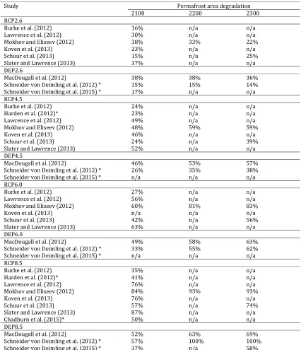
Crucial components of the Earth system, notably the cryosphere and oceans, are highly sensitive to global mean temperature. Indeed, the warming of recent decades has already caused ice sheets to recede globally: the Greenland and Antarctic ice sheets have lost mass, glaciers have continued to shrink almost worldwide, Arctic sea ice and the Northern Hemisphere spring snow have continued to decrease in extent and permafrost temperatures have increased in most regions since the early 1980s (IPCC, 2013). These effects are expected to intensify as warming continues, but projections of their magnitude bear significant uncertainty: by the end of the 21st century, the global glacier volume, excluding glaciers on the periphery of Antarctica, is projected to decrease by 15% to 55% for RCP2.6, and by 35% to 85% for RCP8.5 (IPCC, 2013).
Both the increase in global mean surface temperature and the degradation of ice sheets around the globe will in turn have direct impacts on oceans. So far, oceans seem to have absorbed most of the increase in the energy stored in the climate system, as well as a non-negligible share
4 Scenarios without additional efforts to constrain emissions (‘baseline scenarios’) lead to pathways ranging between
14
of the emitted anthropogenic CO2, which has led to ocean warming5 and acidification6 (IPCC, 2013). The global ocean is expected to continue to warm, which will likely trigger and amplify biophysical processes: the penetration of heat to the deep ocean is expected to affect ocean circulation; ocean thermal expansion and glacier loss will cause sea level rise; and ocean warming will affect sea ice dynamics. Under all RCP scenarios, global mean sea level is expected to rise during the 21st century at rates above those observed between 1971 and 2010, precisely because of ocean warming and increased loss of glacier and ice sheets volume (IPCC, 2013).
Finally, even though the increase in global mean temperature has been used as a metric to summarize the state of Earth’s climate, it says nothing about future local and regional changes in weather. Changes in global mean temperature will have differentiated impacts on temperature, precipitation and wind patterns across the different regions of the world. According to the IPCC, it is virtually certain that most places will experience more hot and fewer cold temperature extremes as global temperatures increase, with the Arctic region expected to warm most (IPCC, 2013). Projections of future precipitation patterns are more hazy: according to current projections, some regions will experience increase and others will experience decreases, while the contrast between wet and dry regions and between wet and dry seasons will increase, although the uncertainties in precipitation projections are larger than for temperature (IPCC, 2013).
There is a general consensus that climate change will increase both the intensity and the frequency of extreme weather events (Herring, Hoerling, Kossin, Peterson, & Stott, 2015; IPCC, 2012). In many land regions, current 1-in-20 year maximum temperature events are expected to become annual or 1-in-2 year events by the end of the 21st century under high-emissions scenarios. Heatwaves are expected to occur with a higher frequency and longer duration (IPCC, 2013). Similarly, extreme precipitation events over wet tropical regions are likely to become more intense and more frequent by the end of the century (IPCC, 2013). There is no clear consensus on the influence of future climate change on tropical cyclones (IPCC, 2013).These co-occurring changes in frequency and intensity could have significant implications for humans and ecosystems: the possibility that changes in the interplay and succession of weather events could cause significant impacts has led to the definition of “compound events”, which have been defined as “extreme impact [events] that depends on multiple statistically dependent variables or events” (Leonard et al., 2014); for instance, these would cover sequences of repeated droughts, periods of very low precipitation co-occurring with high temperatures, or conjoined occurrences of high precipitation events and storm surges.
We mentioned earlier that some components of the climate system could potentially exhibit threshold behaviour (e.g. the collapse of the Atlantic Meridional Overturning Circulation, or the Greenland or West Antarctic ice sheets), which would have potentially severe impacts on human and natural systems. According to the mainstream scientific literature, a 4°C or more increase in global mean temperature compared to pre-industrial times could bring catastrophic climate change, which would manifest itself through tsunamis, extreme sea level rise, desertification of the Sahel region, monsoon disruptions, dieback of the Amazon rainforest, large-scale wildfires in boreal regions and regions disappearing under water (Schellnhuber et al., 2013). There is little information or consensus among scientists on the likelihood of such events
5 The upper 75m of the ocean warmed by 0.11°C per decade over the period 1971 to 2010 (IPCC, 2013).
15
over the 21st century, but most assessments emphasize that the risk of abrupt or irreversible changes increases as the magnitude of the warming increases (IPCC, 2014).
iv. Uncertainties pertaining to the socioeconomic impacts of climate change
Climate change is expected to impact humans and societies through many channels, including agriculture/food, water, health, flooding, natural ecosystems, and even conflict and migration (IPCC, 2014). Both gradual changes and changes in the frequency and severity of extreme weather events will have an impact.
The monetary value of the projected global aggregate impacts of climate change remain highly uncertain: the IPCC estimated that these should remain moderate for a 1 or 2°C warming but are likely to accelerate with increasing temperature, due to the increased risk of regime shifts and biodiversity loss7 accompanying warming of 3°C or more (IPCC, 2014). Unfortunately the majority of the studies of the global aggregate impacts of climate change that can be found in the literature (see Tol, 2009, 2014 for a review) only consider moderate warming, and only 7 studies estimate welfare impacts for warming of 3°C or more (IPCC, 2014). Losses seem to increase sharply with temperature but the uncertainty around these is very high: the most recent estimates project greater impacts than the previous ones and also significantly widened the uncertainty range (IPCC, 2014). We will provide in Section 4 below a more detailed account of the tools and methods that have been devised by economists to estimate these impacts.
These aggregate estimates say nothing about how climate change will impact different countries and populations. However, it is very likely that the impacts of climate change will be felt more strongly by developing countries, both in terms of human and economic impacts.
So far, the human impacts of climate change have been borne predominantly by developing countries: according to the World Health Organization, approximately 60 000 deaths occurred worldwide as a result of weather-related disasters in the 1990s, some 95% of which were in developing countries (World Health Organization, 2017). This is due to a combination of factors including greater exposure, the lack of early warning systems and the absence of available funds for emergency relief and recovery. Unfortunately the situation is likely to get worse in the future: not only will developing countries be the hardest hit by drought-induced food and freshwater shortages, but adverse health impacts, including heat stroke, malaria, dengue and diarrhoea, are also expected to be felt predominantly by low-income countries (UNFCCC, 2010).
Similarly, the economic impacts of extreme weather in the recent past have been incurred predominantly by developing countries: according to a report from the United Nations, the greatest economic losses caused by all weather-related disasters that occurred during the period 1995-2015 were incurred in low-income countries and represented around 5% of GDP (United Nations, 2016). In the round, developing countries are expected to be most vulnerable to future climate change (IPCC, 2014). There are several reasons for this. First, developing countries tend to be geographically located in tropical zones close to the equator, where the effects of climate change will be more negative (IPCC, 2014). For instance, the reduction in the availability of renewable surface water and groundwater is projected to be more acute for dry subtropical
7 According to the Fourth Assessment Report of the IPCC, more than 2 or 3°C warming above preindustrial levels would
16
regions (IPCC, 2014). Second, developing countries are generally more reliant on climate-sensitive sectors (e.g. agriculture and fisheries) than developed countries. Finally, they often have a lower adaptive capacity due to low levels of human capital and technology, limited financial and material resources and unstable or weak institutions (IPCC, 2001a; Lemos et al., 2013). For these reasons climate change could be extremely detrimental to populations at risk in low-income countries, and is expected to prolong existing and create new poverty traps (IPCC, 2014).
But the discrepancy is not only between rich and poor countries: according to the IPCC (2014), the risks related to climate change are expected to be greater for disadvantaged people and communities in countries at all levels of development. Indeed, low-income households usually have a lower adaptive capacity, limited access to insurance and fewer possibilities to relocate to safer accommodation (IPCC, 2014).
The arguments and evidence presented above seem to support the hypothesis that the poor are likely to suffer disproportionate damage from climate change, which, in economic terms, means that the income elasticity of climate change-related damage8 is between 0 and 1. This could have significant implications for the stringency of mitigation at the global level: Dennig et al. (2015) have shown that the optimal level of mitigation is considerably higher when future damage falls especially hard on the poor than when damage is proportional to income. This would also mean that development might be the best defence against climate change impacts (Anthoff & Tol, 2012).
4. What are the methods that have been used by economists to estimate the impacts
of climate change?
We will see in this section the different approaches and methods that have been used by economists to estimate and quantify the impacts of climate change. In his review of the estimates of the welfare effects of climate change, Tol (2009) identified two main approaches: the enumerative method and the (traditional) statistical approach. We will add to these the methods that have been developed since, which include Computable General Equilibrium models, the subjective wellbeing approach and the “New Climate-Economy Literature” (Dell, Jones, & Olken, 2014). Integrated Assessment Models (IAMs), such as DICE (Nordhaus, 1992; Nordhaus & Sztorc, 2013), PAGE (Hope, 2011; Hope, Anderson, & Wenman, 1993), MERGE (Manne, Mendelsohn, & Richels, 1995) and FUND (Tol, 1997), have been used to estimate the impacts of climate change, but can also be considered as policy tools, and will be the topic of the next section.
The enumerative method
These are studies based on the following methodology: projections of the physical impacts of climate change are first obtained from either climate or impact models; these physical impacts are then given a monetary value, and finally added up (enumerated). Despite its apparent simplicity and ease of interpretation, this method suffers from several shortcomings: first, as noted by Fankhauser (2013), this method is based on a partial equilibrium approach, in which the sum of the total damage is the sum of the damage in individual sectors, and does not account for higher-order effects. Then, because it relies on precise sector- and location-specific
17
projections and real market prices, it does not lend itself easily to extrapolation. Finally, because it relies on prices, it is not easily applicable to non-market types of impacts, such as health and biodiversity (Tol, 2009).
The traditional statistical approach
The second group of studies relies on cross-sectional variation in prices and expenditure and how that is associated with cross-sectional variation in climate. This method has been used notably to measure how climate in different places affects the value of farmland (Mendelsohn, Nordhaus, & Shaw, 1994) or per-capita rural income (Mendelsohn, Basist, Kurukulasuriya, & Dinar, 2007). Contrary to the enumerative approach, the statistical approach is based on real-world differences between climate and economic variables and thus it implicitly accounts for adaptation (Tol, 2009). However, cross-sectional studies are at high risk of omitted variable bias, which occurs when the control variables do not account for variables correlated with both the dependent variable and one or more independent variables. This potential bias is a serious challenge for cross-sectional studies as it significantly undermines the ability to make causal inferences, and cannot be easily fixed, as adding control variables can lead to an “over-controlling” problem (Dell et al., 2014).
Computable General Equilibrium models
A third approach to estimating the economic impacts of climate change has made use of Computable General Equilibrium (CGE) models. There were two main reasons that motivated the application of this type of model to climate impacts: the first one is that CGE modelling has enabled economists to address one of the main shortcomings of the enumerative approach, which is the lack of higher-order effects. A few studies have made use of static CGE models to analyse the impacts of climate change on multiple markets (Bosello, Roson, & Tol, 2007; Darwin & Tol, 2001) and most have found that the second-order effects increased the impacts of climate change on welfare (Bowen, Cochrane, & Fankhauser, 2012). In any case, the second-order effects are almost always significant. The second reason, which prompted the use of dynamic CGE models, was the realization of the reverse causation of climate change, i.e. the fact that climate change will be driven by the level of anthropogenic emissions but, at the same time, climate change will affect the economy and thus the level of future GHG emissions; an application of a dynamic CGE model to climate change can be found in Eboli et al. (2010). The limitations of CGE models are twofold: first, since they rely on key parameters which are often arbitrary, they have been criticized for not being sufficiently validated (IPCC, 2001b). Moreover, CGE models can only compare different states of equilibrium and therefore do not provide insight into adjustment processes (IPCC, 2001b).
The subjective wellbeing approach
18
use of happiness data to study economic issues is relatively recent and its application to weather and climate has so far been limited (Carroll, Frijters, & Shields, 2009; Luechinger & Raschky, 2009; Rehdanz & Maddison, 2005). Some methodological issues pertaining to the use of happiness data for environmental valuation have been raised by Welsch and Kuhling (2009) but there are two other factors that limit its applicability to climate change specifically: first, the issue of the spatial and temporal matching of life satisfaction and weather data, which might become problematic in the context of climate change; and second, the substantial challenge posed by the cultural and language components of findings obtained through subjective wellbeing methods, which might significantly impede their external validity.
“The New Climate_Economy Literature” (Dell et al., 2014)
A fifth approach to the estimation of damages from climate change has focused on applying panel data methods to examine how weather variables (mainly temperature, precipitation and windstorms) influence socio-economic outcomes, including agricultural output (Auffhammer & Schlenker, 2014; Deschenes & Greenstone, 2007; Schlenker & Roberts, 2009), production (Hsiang, 2010) and productivity (Burke, Hsiang, & Miguel, 2015). Thorough reviews of this literature can be found in Dell et al. (2014) and Hsiang (2016).
Panel models are generally of the form:
Equation 1.2
𝑦 = 𝛽𝑪 + 𝛾𝒁 + 𝜇 + 𝜃 + 𝜀
Where:
yit is the outcome variable of interest; Cit is a vector of climate variables;
Zit is a vector of other time-varying observables; μi are fixed effects for the spatial areas;
θrt are time fixed effects, which can enter separately by subgroups of the spatial areas to allow for different trends in subsamples of the data (Dell et al., 2014).
19
The main limitations of panel models have to do with how their result can and should be interpreted. The first limitation of panel models is that the inclusion of time fixed effects removes any global effect of weather variations. For instance, panel models such as the one described in the above equation can only provide information on the impact of local, idiosyncratic variations in weather on local outcomes. Spatial spillover effects of a weather shock in a specific region will not be captured by the regression results. One solution to this can be found by dropping the time fixed effects, but this raises the concern that results might be biased by time-varying omitted variables (Dell et al., 2014).
The second limitation of panel models is the question of their external validity in the context of climate change. One of the motivations that spurred this stream of research has been to use these findings on the effect of changes in weather on economic activity, to infer the effects of changes in climate (which can be defined as the average of weather over long time scales) on economic activity. Even supposing that we had access to reliable regional projections of future changes in weather patterns, there are serious limitations to the extrapolation of the findings from these panel models to states of the climate in which Earth’s temperature will be considerably warmer: these restrictions come from the possibility of nonlinearities, potential intensification effects, the eventuality of adaptation, and general equilibrium effects (Dell et al., 2014). For these reasons, the estimates derived from these panel models cannot necessarily be applied to future climate damages: for instance, if adaptation policies are implemented on a large scale, then the effects of current weather shocks might be stronger than the future effects of climate; conversely, if the intensification of weather shocks leads to steep increases in impacts, then estimates derived from current weather shocks could be underestimating the future damages from climate change (Dell et al., 2014). Despite these shortcomings, the emergence of this literature has brought valuable insight.
5. The role of Integrated Assessment Models as policy tools
20
i. Two crucial features of IAMs: the damage function and the discount rate
Because so much information on the Earth’s climate, the global economy and the links between them is condensed in an extremely simple model, IAMs are fraught with structural and parameter uncertainty. This affects many relationships and parameters in IAMs but three components have come under particular scrutiny: the equilibrium climate sensitivity, the damage function and the discount rate (Farmer, Hepburn, Mealy, & Teytelboym, 2015; Stern, 2013). We have mentioned in Section 2 the uncertainty surrounding the equilibrium climate sensitivity as well as the notion of “fat tails”, so we will focus here on the two key economic components of IAMs, the damage function and the discount rate.
The damage function
The first key economic component of IAMs is the damage function, which is a measure of the relative impact on welfare (expressed in terms of GDP) of an increase in global mean temperature, as an index of a wider set of climatic changes. Since climate change is an unprecedented phenomenon in the history of mankind, there are no historical observations available, which could inform the “shape” of this relationship; damage functions thus belong to the realm of the structural uncertainties and result from largely arbitrary choices.
The damage function in the DICE Integrated Assessment Model is quadratic in global mean temperature change. Previously, this damage function was calibrated based on the enumerative approach, involving detailed regional and sectoral estimates (Nordhaus & Boyer, 2000), but in DICE-2013R (Nordhaus & Sztorc, 2013), a most recent version of the model, the calibration of the damage function is based on the estimates of monetized damages from the Tol survey (Tol, 2009, 2014), to which a judgemental 25% adjustment is added to reflect non-monetized impacts, such as biodiversity losses, health impacts and changes in ocean circulation.
Equation 1.3
𝛺 𝑇𝐴𝑇𝑀(𝑡) = 1
1 + 𝛼 ∗ 𝑇𝐴𝑇𝑀(𝑡) + 𝛼 ∗ (𝑇𝐴𝑇𝑀(𝑡))
Where:
TATM is the increase in global mean temperature since pre-industrial times (in °C); α1 = 0;
α2 = 0.002664.
There are two important issues with this damage function. The first issue regards the choice of a quadratic specification, which is essentially arbitrary: as noted by Dietz and Asheim (2012, p. 328), “there has never been any stronger justification for the assumption of quadratic damages than the general supposition of a non-linear relationship, added to the fact that quadratic functions are of a familiar form to economists, with a tractable first derivative”9. The second issue concerns the calibration of this damage function: not only is it designed so that damages cannot reach 100% of output, but its calibration is only valid for temperature increases
9 It is worth noting here that, in contrast to most IAMs, the impact function in PAGE09 has a flexible exponent that can
21
in the range of 0 to 3°C. Indeed, the damage function used in DICE means that a 6°C increase in global mean temperature warming would result in a loss of utility equivalent to just 4.7% of output, while it would take an 18°C increase in global mean temperature to reach a loss of utility equivalent to 50% of output (Ackerman, Stanton, & Bueno, 2010; Dietz & Asheim, 2012). Hence several economists have expressed their concerns about the choice of a quadratic damage function that might significantly understate the economic impacts associated with very large increases in global mean temperature (Ackerman et al., 2010; Pindyck, 2013; Stern, 2013; Weitzman, 2011). The third issue pertains to the fact that the damage function used in DICE-2013R does not include thresholds, and therefore does not account for the possibility of tipping points, regime shifts, or the possibility of catastrophic climate change (Lemoine & Traeger, 2014).
The structural uncertainty about the specification of the damage function has been dealt with in three ways: the first one has been to keep the base relationship and to introduce a higher-order term into the damage function to capture greater non-linearity (Weitzman, 2011). To that effect, Dietz and Asheim (2012) transformed this structural uncertainty into a parametric uncertainty by proposing the use of a damage function which is such that, for different parameter values, the damage function can be equivalent either to the quadratic form of Nordhaus (2014), or that of Weitzman (2012). They interpret the parametric uncertainty as being subjective or epistemic in nature, rather than objective or aleatory.
The second approach has been to question the assumption that damages do not enter the utility function directly, which supposes that there is a strong substitutability between consumption and the costs of temperature change. Instead, Weitzman (2009a, 2011) has suggested to make the disutility of temperature change additively separable from the utility of consumption, which would reflect the fact that climate change might have impacts (e.g. on biodiversity, ecosystems and human health) which are not readily substitutable with material wealth.
The third approach has been to replace the damage function in which economic impacts of climate change hit current year GDP losses by a damage function which better reflects the scale and long-lasting effects of climate damage. To this effect, Stern (2013) has suggested alternative damage functions, where climate damage could be modelled as 1) damage to social, organizational or environmental capital; 2) damage to stocks of capital or land; 3) damage to overall factor productivity; 4) damage to learning and endogenous growth. Some of these recommendations have since been implemented: Moyer et al. (2014) integrated in the DICE model the possibility that climate change may directly affect productivity. Similarly, Moore and Diaz (2015) adapted DICE so that temperature could affect GDP through two pathways: total factor productivity growth and capital depreciation. Finally, Dietz and Stern (2015) incorporate in DICE two models of endogenous growth, in which the damage from climate change affect the drivers of long-run growth.
The discount rate
22
maximum warming response is a decade on average (Ricke & Caldeira, 2014; Zickfeld & Herrington, 2015), CO2 emissions are long-lived: on average 40% of a CO2 pulse is still in the atmosphere after 100 years (Ciais et al., 2013). This means that an emission today produces a stream of impacts for centuries, and that the net present value of the total impact is heavily influenced by the choice of the discount rate. Consequently, the costs of an abatement policy would be incurred as of now, but that most of the benefits would occur at uncertain horizons and in the long distant future. Given the timescales involved, the choice of a discount rate can therefore make an immense difference in the net present value of future costs and benefits.
In the discounted utilitarian framework, which is the one used in DICE, social welfare is represented by the sum of the utility of a representative agent:
Equation 1.4
𝑈 𝑐(𝑡) = 𝑢[𝑐(𝑡)] exp(−𝜌𝑡) 𝑑𝑡
where the instantaneous utility function u[c(t)] is time invariant and has positive but diminishing marginal utility of consumptions (i.e. u’(.) > 0 and u’’(.) ≤ 0).
Assuming that we are in a risk-free setting, that the utility function is iso-elastic and that we are in an economy where capital yields output, which can be devoted to consumption or investment, the maximisation10 of the above equation leads to the Ramsey rule (Ramsey, 1928):
Equation 1.5
𝑟 = 𝜌 + 𝜃𝑔
Where:
r is the social marginal productivity of capital;
ρ is the utility discount rate or the pure rate of time preference; θ is the coefficient of risk aversion or the elasticity of marginal utility; 𝑔 = ̇( )( ) is defined as the growth rate of consumption.
The uncertainty about what would be the “appropriate” discount rate in the context of climate change stems from at least two factors: first, whether the components of the discount rate (namely the rate of pure time preference and the consumption elasticity of marginal utility) should be taken from a normative or a positive perspective. For instance, Ramsey (1928, p. 543) argued that putting different weights upon the utility of different generations is “ethically indefensible” while Stern (2007) defends the use of a pure rate of time preference of 0.1 to account for the small risk of extinction of the human race, but otherwise rules out impatience as a legitimate motivation for pure-time discounting. Nordhaus (2007) has taken the opposite view and has argued that discount rates should be derived from actual behaviour, which means that the ρ parameter should be inferred from empirical estimates of market rates of return.
The second factor concerns the uncertainty about future consumption growth. Assuming that that there is uncertainty about consumption growth and that the growth rate of consumption
23
is independently and identically normally distributed with mean μ and variance σ2, a third term, called the precautionary effect, is added to Equation 1.5, which becomes the extended Ramsey rule (Equation 1.6).
Equation 1.6
𝑟 = 𝜌 + 𝜃𝜇 − 0.5𝜃 𝜎
In the Ramsey framework, the presence of uncertainty about the future rate of growth in per capita consumption justifies a declining discount rate (Gollier, 2002), if we make the assumption that the utility function is isoelastic and that shocks in consumption are positively correlated (Cropper, Freeman, Groom, & Pizer, 2014).
It is worth emphasizing that at the core of the discounted utilitarian framework lies the assumption that the utility of future generations should be given less weight than the utility of the present generation, which becomes crucial when it comes to evaluating climate policies (Dietz & Asheim, 2012). Although they are not explored in this thesis, alternative approaches to the discounted utilitarian framework have been proposed in the literature; these include for instance sustainable discounted utilitarianism (Asheim & Mitra, 2010) and the rank-discounted utilitarian approach (Zuber & Asheim, 2012).
ii. Limitations of Integrated Assessment Models
Three issues with the representation of uncertainty in IAMs have been raised in the literature: IAMs have difficulty in accounting for the possibility of catastrophic climate change, they generally cannot provide detailed projections of regional impacts, and they present an illusion of certainty which can be misleading to some.
The first concern regarding the reliability of IAM-derived projections lies in the fact that these do not seem to reflect the findings of climate scientists regarding the range of future states of the climate, mainly due to the absence of positive feedbacks and tipping points (Kaufman, 2012; Lenton & Ciscar, 2013; Warren, Mastrandrea, Hope, & Hof, 2010). This claim has been substantiated by the work of Ackerman et al. (2010), who examined the conditions under which DICE could project forecasts of disastrous climate outcomes and found that it required a conjunction of a fat-tailed distribution for the equilibrium climate sensitivity parameter and the specification of the damage function. One of the responses to this concern has been to integrate the possibility of a climate catastrophe in IAMs through tipping points (Lemoine & Traeger, 2016; Lenton & Ciscar, 2013; Lontzek, Cai, Judd, & Lenton, 2015). A different standpoint was taken by Weitzman (2009b), who laid out the Dismal Theorem which argues that the large structural uncertainty surrounding the possibility of a climate catastrophe renders obsolete the use of standard cost-benefit analysis.
The second critique of IAMs that can be found in the literature is that most of them operate on a global scale, and therefore say nothing on the local impacts of climate change on lives and livelihoods. Some regional IAMs have been developed11 but these suffer from two drawbacks: first, reliable projections of regional climatic changes do not in general exist, except perhaps for warming; second, these impacts will also depend very strongly on local socio-economic factors
24
which are extremely hard to project, such as the implementation of adaptation policies and changes in vulnerability and resilience. The fact that most IAMs rely on the assumption of a representative agent (Farmer et al., 2015) also forecloses the possibility of including heterogeneous agents (Beinhocker, Farmer, & Hepburn, 2013).
The final objection that has been made is that IAMs can, if not used with care, give an illusion of knowledge to policy-makers who use their output. It is true that IA modellers have considerable freedom in choosing functional forms and parameter values, which can lead to very different estimates of the social cost of carbon and the optimal policy; this highlights the fragility of these models to the underlying specifications but is not a major issue in itself. What is wrong and dangerous is to consider the results from these models as certain, without acknowledging the wide uncertainties underlying them and the numerous assumptions that these results depends on. In the words of Pindyck (2017, p. 102) : “the use of IAMs to estimate the SCC or evaluate the alternative policies is problematic because it creates a veneer of scientific legitimacy that is misleading”.
What then should be the purpose of IAMs? Integrated Assessment Models should be used as analytical devices, designed to bring a better understanding of the dynamic interactions between climate change and the economy and to compare different mitigation scenarios in relative terms. IA modellers should resist the demands of policy-makers for scientific-looking probability distributions of future climate impacts, and instead acknowledge the depth of our ignorance, and precisely use these models to explore the full range of climate and economic uncertainties, and the ways in which these combine and compound.
All in all, what matters ultimately in the context of climate change is the probability of catastrophic climate change and the scale and nature of regional impacts, for which IAMs are of limited use anyway. Alternative methods have thus been developed to address more precisely these issues.
iii. Alternative approaches to IAMs
Four approaches have been used in the field of climate change to deal with the weaknesses and shortcomings of Integrated Assessment Models: expert elicitation, aimed at facilitating the characterization of deep uncertainty; closed-form analytical solutions, meant to replicate IAMs’ outputs with simple and transparent formulae; dynamic stochastic general equilibrium model, which allow for stochastic elements in the path to the steady state; and agent-based models, which answer the need to take into account the heterogeneity of agents.
Expert elicitation
25
level rise from ice sheets (Bamber & Aspinall, 2013), the likelihood of tipping points (Lenton et al., 2008) and the strength of the permafrost carbon feedback (Schuur et al., 2013). Pindyck (2016) suggests that instead of relying on IAMs to project future economic impacts of climate change, we should rely on expert opinion to elucidate the likelihood of a catastrophe (which is, in the end, the major determinant of the economic value of mitigation). There are several limitations to this method: the first one lies in the fact that the potential pool of experts for these types of survey is extremely small; second, the likelihood assessments provided by these experts might be constructed in very different ways, from heuristic methods to model simulations; third, though representative of the range of beliefs about the likelihoods of catastrophic climate change, the aggregated results of the survey cannot be treated as a consensus probability distribution (Arnell, Tompkins, & Adger, 2005). Finally, the human brain has been shown to be prone to heuristics which can significantly influence judgments (Tversky & Kahneman, 1975).
Closed-form analytical solutions
A second approach has tried to provide similar, policy-relevant results to the ones provided by IAMs (e.g. the optimal level of mitigation or the social cost of carbon), but using closed-form analytical formulae. IAMs are often criticised for their lack of transparency and the fact that they operate as “black boxes”. There are two prominent examples in the recent literature. Golosov et al. (2014) found that, under a certain set of assumptions, the calculations leading to the optimal carbon tax in a dynamic stochastic general equilibrium model could be synthetized into a closed-form analytical formula. The main advantage of this solution lies in the fact that it only depends on a few basic parameters, namely, assumptions on discounting, a measure of expected damages and how fast emitted carbon leaves the atmosphere. Moreover, it should be palatable to policy-makers, as its simplicity makes it easy to understand and its outcome does not rely on calculations happening behind the scenes. A similar approach was used by van den Bijgaart et al. (2016), who derived a closed-form analytical solution for the social cost of carbon. The authors compared the performance of their formula against the DICE IAM and found that their formula predicts the outcome from DICE without quantitatively significant systematic bias.
Dynamic stochastic general equilibrium models
A third approach has tried to improve the treatment of uncertainty by combining IAMs with Dynamic Stochastic General Equilibrium (DSGE) methods. For instance, Traeger (2014) transformed DICE into a recursive dynamic programming model, so as to be able to incorporate stochastic shocks, persistent uncertainty and Bayesian learning. The main advantage of DSGE models is that they enable a more thorough integration of uncertainty but they are usually computationally intensive and rely on the assumption of forward-looking fully-informed maximising agents (Farmer et al., 2015).
Agent-based models
26
additional instruments (e.g. diffusion of information and lifestyles), and addressing Schumpeterian competition (through innovation, rather than price competition). It has been argued that the use of ABM would be especially salient in the context of climate change, as population groups are expected to be impacted differently by the opportunities and threats posed by mitigation policies (S. Moss, Pahl-Wostl, & Downing, 2001). However, the use of ABMs comes at the cost of considerable computational needs and they usually require the empirical estimation of a significant number of parameters.
6. Dissertation outline
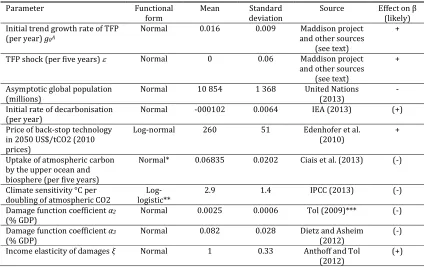
The second chapter of my PhD, titled “The climate beta”, and co-written with Pr. Simon Dietz and Pr. Christian Gollier, investigates the discount rate that should be applied to mitigation projects through the prism of the climate beta, i.e. the correlation between the returns of a mitigation project and future consumption growth. We start by exploring analytical properties of the climate beta, before estimating it numerically using the Integrated Assessment Model DICE. The fact that I had to code DICE from scratch in Matlab gave me a sound understanding of the calculations going on in the “black box” and made me aware of the considerable structural and parameter uncertainties which underlie these models. Given that our analysis examines the impact of uncertainty about the climate beta, I also had to find sensible probability distribution functions for ten key uncertainties, including the rate of CO2 uptake by the ocean, the notion of equilibrium climate sensitivity and the curvature of the damage function, which provided me with both a wide and a precise knowledge of climate change uncertainties.
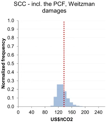
Delving into the notion of equilibrium climate sensitivity made me reflect on the crucial role played by feedbacks in the response of the Earth’s climate to an increase in radiative forcing, which led me to the third chapter of my PhD: “Estimating the economic impact of the permafrost carbon feedback”. In this chapter, I explore the impact of integrating the permafrost carbon feedback in the Integrated Assessment Model DICE. The complexity came from finding a simple and yet informative representation of this biogeophysical feedback, which could be incorporated in DICE so as to assess its potential impact on the social cost of carbon and the optimal climate policy.
27
28
R
EFERENCESAckerman, F., Stanton, E. A., & Bueno, R. (2010). Fat tails, exponents, extreme uncertainty: Simulating catastrophe in DICE. Ecological Economics, 69(8), 1657-1665.
Anthoff, D., & Tol, R. S. (2012). Schelling’s conjecture on climate and development: a test. Climate change and common sense: essays in honour of Tom Schelling, 260-275.
Arnell, N. W., Tompkins, E. L., & Adger, W. N. (2005). Eliciting information from experts on the likelihood of rapid climate change. Risk Analysis, 25(6), 1419-1431.
Arrhenius, S. (1896). XXXI. On the influence of carbonic acid in the air upon the temperature of the ground. The London, Edinburgh, and Dublin Philosophical Magazine and Journal of Science, 41(251), 237-276.
Asheim, G. B., & Mitra, T. (2010). Sustainability and discounted utilitarianism in models of economic growth. Mathematical Social Sciences, 59(2), 148-169.
Auffhammer, M., & Schlenker, W. (2014). Empirical studies on agricultural impacts and adaptation. Energy Economics, 46, 555-561.
Bamber, J. L., & Aspinall, W. (2013). An expert judgement assessment of future sea level rise from the ice sheets. Nature Climate Change, 3(4), 424.
Beinhocker, E. D., Farmer, J. D., & Hepburn, C. (2013). Next generation economy, energy and climate modeling. Global Commission on Economy and Climate, 11.
Bosello, F., Roson, R., & Tol, R. S. J. (2007). Economy-wide Estimates of the Implications of Climate Change: Sea Level Rise. Environmental and Resource Economics, 37(3), 549-571. Bowen, A., Cochrane, S., & Fankhauser, S. (2012). Climate change, adaptation and economic
growth. Climatic Change, 113(2), 95-106.
Burke, M., Hsiang, S. M., & Miguel, E. (2015). Global non-linear effect of temperature on economic production. Nature, 527(7577), 235-239.
Calel, R., Stainforth, D. A., & Dietz, S. (2015). Tall tales and fat tails: the science and economics of extreme warming. Climatic Change, 132(1), 127-141.
Carroll, N., Frijters, P., & Shields, M. A. (2009). Quantifying the costs of drought: new evidence from life satisfaction data. Journal of Population Economics, 22(2), 445-461.
Cette, G., Lecat, R., & Ly-Marin, C. (2017). Long-term growth and productivity projections in advanced countries.
Ciais, P., Sabine, C., Bala, G., Bopp, L., Brovkin, V., Canadell, J., . . . Heimann, M. (2013). Carbon and other biogeochemical cycles. In Climate change 2013: the physical science basis.
Contribution of Working Group I to the Fifth Assessment Report of the Intergovernmental Panel on Climate Change (pp. 465-570): Cambridge University Press.
Cropper, M. L., Freeman, M. C., Groom, B., & Pizer, W. A. (2014). Declining discount rates. The American Economic Review, 104(5), 538-543.
Cuñado, J., & de Gracia, F. P. (2013). Environment and Happiness: New Evidence for Spain. Social Indicators Research, 112(3), 549-567.
Darwin, R. F., & Tol, R. S. (2001). Estimates of the economic effects of sea level rise. Environmental and Resource Economics, 19(2), 113-129.
Dell, M., Jones, B. F., & Olken, B. A. (2014). What Do We Learn from the Weather? The New Climate-Economy Literature. Journal of Economic Literature, 52(3), 740-798. Dennig, F., Budolfson, M. B., Fleurbaey, M., Siebert, A., & Socolow, R. H. (2015). Inequality,
climate impacts on the future poor, and carbon prices. Proceedings of the National Academy of Sciences, 112(52), 15827-15832.
Deschenes, O., & Greenstone, M. (2007). The economic impacts of climate change: evidence from agricultural output and random fluctuations in weather. The American Economic Review, 97(1), 354-385.