The London School of Economics and Political Science
Historical Events and their Effects on
Long-Term Economic and Social
Development
Maria Waldinger
A thesis submitted to the Department of International Development
of the London School of Economics for the degree of Doctor of Philosophy
2
Declaration
I certify that the thesis I have presented for examination for the MPhil/PhD degree of the London School of Economics and Political Science is solely my own work other than where I have clearly indicated that it is the work of others (in which case the extent of any work carried out jointly by me and any other person is clearly identified in it).
The copyright of this thesis rests with the author. Quotation from it is permitted, provided that full acknowledgement is made. This thesis may not be reproduced without my prior written consent.
I warrant that this authorisation does not, to the best of my belief, infringe the rights of any third party.
London, 03 July 2014
3
Abstract
This thesis uses econometric methods to examine the effects of historical events and developments on aspects of economic and social development. Its objective is two-fold: The thesis examines causes and effects of different historical events using econometric methods and newly constructed and newly available data sets. By studying these historical events, broader theoretical questions are addressed that are relevant and have implications for today.
The first chapter studies the economic effects of the Little Ice Age, a climatic period that brought markedly colder conditions to large parts of Europe. The theoretical interest of this study lies in the question whether gradual temperature changes affect economic growth in the long-run, despite people’s efforts to adapt. This question is highly relevant in the current debate on the economic effects of climate change. Results show that the effect of temperature varies across climate zones, that temperature affected economic growth through its effect on agricultural productivity and that cities that were especially dependent on agriculture were especially affected.
The second chapter examines the role of adverse climatic conditions on political protest. In particular, it assesses the role of adverse climate on the eve of the French Revolution on peasant uprisings in 1789. Historians have argued that crop failure in 1788 and cold weather in the winter of 1788/89 led to peasant revolts in various parts of France. I construct a cross section data set with information on temperature in 1788 and 1789 and on the precise location of peasant revolts. Results show that adverse climatic conditions significantly affected peasant uprisings.
4
Acknowledgements
I would like to thank my advisor Diana Weinhold for her steady encouragement over the past years, and Daniel Sturm for his valuable guidance and advice. I also thank researchers at LSE and Harvard University who have provided valuable comments on my work.
I am very grateful for the financial support and encouragement I received from Cusanuswerk since my undergraduate studies and especially during the PhD.
I thank my family, Gunter, Marlies, Astrid, Gregor, Bernward, and Elisabeth, for the wonderful bond between us.
I dedicate this thesis to my parents Marlies and Gerhard Fleischhauer and to their endless love for us.
5
Preface
This thesis examines econonometrically causes and effects of historical events. The purpose of this approach is two-fold: First, this thesis contributes to historical research, in particular by using econometric methods to analyse newly available or newly constructed data. Thereby, the thesis sheds new light on historical debates. At the same time, by studying historical events, each chapter also addresses theoretical questions that have important implications for today.
In the first chapter, I study the effects of climatic change during the Little Ice Age on economic growth in Early Modern Europe. Historians have provided anecdotal evidence that relatively cold temperature during the Little Ice Age had a negative effect on the economy (e.g Fagan, 2000; Behringer 2010). This is the first study to provide econometric evidence on the economic effects of the Little Ice Age studying all of Europe. It thereby contributes to research in climate history and to research on the economic growth experience of Early Modern Europe. At the same time, this chapter also addresses a broader theoretical question by providing econometric evidence on the economic effects of long-term climate change, when climate change spans several centuries and people have time to adapt. This question is highly relevant in the current debate on climate change and to date empirical evidence is scarce. The question of which rate of adaptation can be realistically assumed in current climate models is especially urgent. This chapter provides evidence that the effect of climate change is highly context-specific. Better access to trade, for example, decreases vulnerability to climate change.
6 weather events. At the same time, this study contributes to the well-known hypothesis that the drought summer of 1788 and the harsh winter of 1788/89 had a direct effect on peasant uprisings by causing food insecurity. I use newly available paleoclimatological data to shed new light on this question. This chapter is also the first econometric test of this hypothesis. The econometric approach allows to establish causality between temperatures and uprisings by exploiting variation in weather within France and variation in the outbreaks of peasant uprising across France and variation in their timing. As in the previous chapter, this chapter examines a historical research question while at the same time contributing to our understanding of the theoretical relationship between weather shocks and uprisings.
The third chapter studies the long-term effects of missionaries in colonial Mexico on educational and cultural outcome variables. It contributes to the strand of literature on the long-term effects of missionaries by refining the definition of missionaries that has been used in previous studies and by introducing instrumental variable estimation addressing the notorious identification problem that stems from the endogenous location of mission stations. At the same time, this chapter contributes to our knowledge on the long-term transmission of cultural values. By studying different missionary order separately, it shows that only those orders with corresponding values had lasting effects on educational outcomes.
7
Table of Contents
Declaration………. ... 2
Abstract……. ... 3
Acknowledgements ... 4
Preface………. ... 5
Table of Contents ... 7
List of Tables ... 10
Table of Figures ... 12
1. The Long Term Effects of Climatic Change on Economic Growth: Evidence from the Little Ice Age, 1500 – 1750 ... 13
1.1. Introduction ... 13
1.2. The Effect of the Little Ice Age on Agricultural Productivity and Urban Growth ... 18
1.3. Data ... 24
1.4. Empirical Strategy ... 31
1.5. Baseline Results ... 32
1.6. Robustness ... 38
1.7. The Role of Agricultural Productivity ... 48
1.8. Heterogeneity in the Effect of Temperature ... 55
1.2.1. The Little Ice Age ... 18
1.2.2. Effect of the Little Ice Age on agricultural productivity ... 19
1.2.3. Effect of agricultural productivity on economic and population growth . 19 1.2.4. Effect of agricultural productivity on city growth and urbanisation ... 22
1.5.1. Basic Results and Geographic Controls ... 32
1.5.2. Controlling for Historical Determinants of Economic Growth ... 34
1.5.3. The Effect of Temperature on Urbanisation ... 37
1.6.1. Alternative Samples ... 38
1.6.2. Alternative Fixed Effects and Time Trends ... 41
1.6.3. Using Alternative Standard Errors ... 42
1.6.4. The Effect of Temperature in Different Climate Zones ... 44
1.7.1. The Effect of Temperature on Wheat Prices ... 48
8
1.9. Comparability to Current Economic Situation ... 67
1.10. Conclusion ... 71
2. Drought and the French Revolution: The effect of economic downturn on peasant revolts in 1789 ... 74
2.1. Introduction ... 74
2.2. Political, Economic, and Intellectual Context before 1789 ... 77
2.3. Theoretical and Historical Framework ... 83
2.4. Empirical Strategy and Data ... 88
2.5. Empirical Results ... 95
2.6. Conclusion ... 113
3. Missionaries and Development in Mexico ... 116
3.1. Introduction ... 116
3.2. Historical Background ... 118
3.3. Data Sources and Data Set Construction ... 128
3.4. Results ... 133
1.8.1. The Effect of Temperature on Small and Large Cities ... 55
1.8.2. The Effect of Temperature on Trade Cities ... 58
1.8.3. The Effect of Temperature Conditional on City Size and Trade Estimated Using Interaction Terms ... 62
2.3.1. The elite and the disenfranchised in French society in 1789 ... 84
2.3.2. Collective action by the disenfranchised ... 85
2.3.3. The de facto political power of the disenfranchised vs. the elite’s military force ... 85
2.3.4. Revolution during Recession ... 87
2.3.5. Peasant Revolt and Institutional Reform ... 87
2.4.1. Data Description ... 88
2.4.2. Empirical Strategy ... 93
2.5.1. Basic Specifications ... 95
2.5.2. Augmented Specifications ... 98
2.5.3. Testing for an Effect of Temperature Deviations in Earlier Years ... 103
2.5.4. Temperature, Peasant Revolt, and Different Economic Sectors... 106
2.5.5. Exploring Temperature’s Direct Effect on Agricultural Productivity .... 111
3.2.1. Mexico in 1524 ... 118
9
3.5. Robustness ... 139
3.6. Instrumental Variable Estimation – Early Directions and Missionary Momentum ... 143
3.7. Conclusion ... 159
4. Bibliography ... 162
3.5.1. Results within Mission Area ... 139
3.5.2. Altonji-Elder-Taber statistics ... 141
10
List of Tables
Table 1 Summary Statistics ... 28
Table 2 Climate Groups & Corresponding Koeppen-Geiger Climate Groups ... 30
Table 3 The Effect of Temperature on City Size - Baseline Estimates and Geographic Controls ... 33
Table 4 Robustness Additional Historical Control Variables... 36
Table 5 The Effect of Temperature on Urbanisation ... 38
Table 6 The Effect of Temperature on City Size - Different Samples ... 40
Table 7 Fastest Growing Cities in Europe in 1600 ... 41
Table 8 Alternative Fixed Effects and Time Trends ... 42
Table 9 Robustness Using Alternative Standard Errors ... 43
Table 10 The Effect of Temperature in Different Climate Zones ... 47
Table 11 The effect of yearly temperature on yearly wheat prices - all cities ... 51
Table 12 The effect of yearly temperature on yearly wheat prices – by city ... 52
Table 13 The effect of yearly temperature on yearly yield ratios... 54
Table 14 The Effect of Temperature in Small and Large Cities ... 57
Table 15 Cities of the Hanseatic League ... 59
Table 16 The Effect of Temperature on Cities of the Hanseatic League ... 61
Table 17 Regression Equations and Interaction Terms For Table 18 ... 65
Table 18 The Effect of Temperature on Cities Conditional on Climate, City Size, and Hanseatic League Membership ... 66
Table 19 The effect of temperature on city size in… ... 67
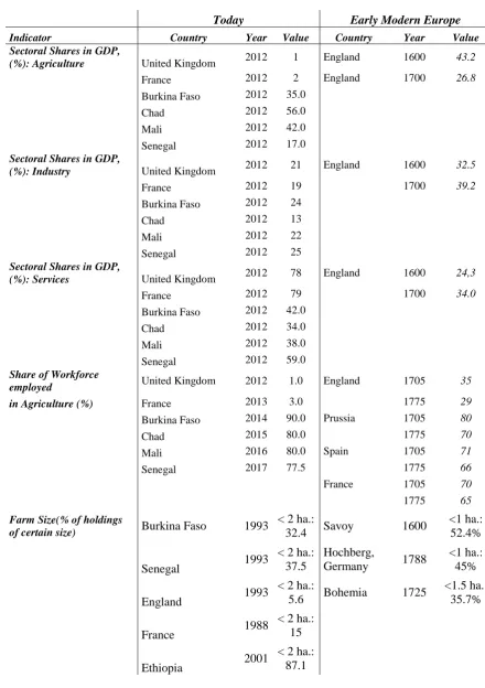
Table 20 Economic characteristics of Countries in Early Modern Europe and Today ... 70
Table 21 Summary Statistics ... 92
Table 22 Peasant Revolts and Extreme Temperatures – Basic Results ... 96
Table 23 Peasant Revolts and Deviations from Long-Term Mean Temperature – Basic Results ... 98
Table 24 Peasant Revolts and Extreme Temperatures – Augmented Specifications ... 101
Table 25 Peasant Revolts and Deviations From Long-Term Mean Temperature - Augmented Specifications ... 102
Table 26 Testing for an Effect of Temperature Deviations on Peasant Revolts in Earlier Years ... 105
11
Table 28 Peasant Revolts, Temperature and Manufacturing ... 110
Table 29 Effect of Temperature Deviations on Froment (Wheat) Prices ... 113
Table 30 The Orders’ Principles and Excerpts from their Rules ... 126
Table 31 Summary Statistics ... 130
Table 32 Summary Statistics - Comparision of Differences in Means of Pre-Colonial Variables ... 132
Table 33 The Aggregate Effect of Orders on Outcomes ... 134
Table 34 The Effect of Mendicant and Jesuit Orders on Outcomes ... 135
Table 35 The Effect of Mendicant and Jesuit Orders Including Municipality Fixed Effects ... 136
Table 36 The Effect of Each Order Separately on Outcomes ... 138
Table 37 The Effect of Each Order Separately Including Municipality Fixed Effects ... 139
Table 38 OLS Results Within Mission Areas ... 139
Table 39 OLS Results Within Mission Areas Municipality Fixed Effects ... 140
Table 40 OLS Results Per Order Within Mission Areas ... 140
Table 41 OLS Results Per Order Within Mission Areas Municipality Fixed Effects ... 141
Table 42 Altonji-Elder-Taber statistics δ-values ... 142
Table 43 The Orders' Early Directions ... 144
Table 44 The Effect of Mendicant and Jesuit Orders with Different Control Variables ... 150
Table 45 First Stages Regressions ... 151
Table 46 Instrumental Variable Regression Results ... 154
12
Table of Figures
Figure 1 Temperature and City Size, 1600 ... 26
Figure 2 European annual mean temperature, 20 year moving average ... 27
Figure 3 European annual mean temperature as 20 years moving averages, according to latitude ... 29
Figure 4 European Climate Groups ... 45
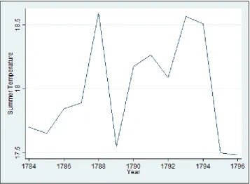
Figure 5 Mean summer temperature for France between 1784 and 1796 ... 82
Figure 6 Peasant Revolts, July - August 1789 ... 91
Figure 7 Catholic Mission Stations in Colonial Mexico by Order 1524 – 1810 Catholic ... 121
Figure 8 Establishment of Missions and of Spanish Military Control in 1540, 1580 and 1700 ... 124
Figure 9 First 10 Dominican Missions in Mexico and Final Distribution ... 146
Figure 10 First 10 Augustinian Missions in Mexico and Final Distribution ... 147
Figure 11 First 10 Franciscan Missions in Mexico and Final Distribution ... 148
Figure 12 First 10 Jesuit Missions in Mexico and Final Distribution ... 149
13
1.
The Long Term Effects of Climatic
Change on Economic Growth: Evidence
from the Little Ice Age, 1500 – 1750
1.1.
Introduction
Obtaining a realistic estimate of the long term effect of global warming on economic growth is crucial for identifying efficient policy responses. One strand of literature, e.g. the influential Stern Review (Stern, 2007) estimates the economic cost of climate change based on Integrated Assessment Models. They specify and quantify an array of mechanisms through which climatic change may affect national income. This approach has received considerable public attention and has informed important policy choices. A criticism of this approach is that the complex relationships between climate and the economy are extremely challenging to capture in its entirety (Dell et al., 2012: 67). Results depend on a large number of assumptions whose validity is very difficult to test. One source of uncertainty is the degree of adaptation that could realistically be assumed (Stern, 2007: 149).
Another strand of literature explores empirically the effects of year-to-year fluctuations in temperature on economic outcomes (Dell et al., 2012; Burgess et al., 2011; Deschenes and Greenstone, 2007, 2012). Yet, the authors point out that the effects of short-term temperature fluctuations are likely to be different than the effects of long-term temperature change because the empirical framework does not include the possibly important role of adaptation.
14 throughout Europe [...] shortened growing seasons led to reductions in agricultural productivity [...],” (Aguado et al., 2007: 483). Famines became more frequent (Behringer, 2005: 226).
To assess the long term effect of temperature change on economic growth I construct a panel data set for over 2000 European cities. These data measure annual temperature between 1500 and 1750 and city size data for several points in time. The temperature data for each city come from a large temperature reconstruction effort that was undertaken by climatologists (Luterbacher et al., 2004). The data set contains gridded ‘temperature maps’ for each year since 1500 that cover all of Europe. Each grid cell measures ca. 50 by 50 kilometres which allows for a precise measurement of climatic change at the local level. The temperature data are reconstructed using directly measured temperature for later years, temperature indices from historical records as well as proxy temperature reconstructions from ice cores and tree ring series (Luterbacher et al., 2004: 1500). As a proxy for economic growth I use data on historical city sizes for over 2,000 European cities that are obtained from Bairoch (1988) and data on country-level urbanisation that are defined based on work by McEvedy and Jones (1978) and Bairoch (1988).
The main analysis investigates the effect of temperature on city size and on urbanisation proxies for economic growth. To control for other factors that may have affected long-run economic growth I control for city fixed effects and country times year fixed effects. City fixed effects control for each city’s time invariant characteristics, such as geographic characteristics or persistent cultural traits.
15 ruggedness (Benniston et al. 1997) I also control for elevation and ruggedness. Then, I control for a number of historical determinants of city size in Early Modern Europe that have received particular attention in the literature: being part of an Atlantic trading nation (Acemoglu, Johnson, and Robinson, 2005), majority Protestant in 1600 (Becker and Woessmann, 2009), a history of Roman rule and access to Roman roads (Landes, 1998), being a university town (Cantoni et al. 2013), distance to battlegrounds (Dincecco et al. 2013), and distance to the coast. Finally, I show that the results are robust to the use of Conley (1999) standard errors that assume spatial autocorrelation between observations, to the inclusion of period-specific country border fixed effects, period-specific country border time trends, and city time trends.
Then, I investigate heterogeneity in the effect of temperature. Results show that temperature had a nonlinear effect on city size. During the Little Ice Age, when temperature was relatively low, temperature increases had an overall positive effect on city size, especially in cold areas. The effect of temperature changes on economic growth is heterogeneous across climate zones. In parts of Europe with a hot and dry climate, especially in southern Spain, further temperature increases led to lower growth. I also investigate temperature’s effect on agricultural productivity. I combine yearly temperature data with yearly wheat prices for ten European cities over a period of ca. 300 years starting in 1500 (Allen, 2003). As city level demand changes only gradually yearly fluctuations in wheat prices are likely to be a reflection of changes in supply. My analysis indicates that rising temperatures are associated with falling wheat prices in northern cities and with rising wheat prices in southern cities. This pattern of results suggests that temperature changes were related to changes in agricultural output which then affected city size. Then, I then introduce yield ratios as a direct measure of agricultural productivity (based on Slicher van Bath, 1963). Consistent with previous results,results show that higher temperatures increased yield ratios, and hence agricultural productivity.
16 cushion the blow through the existence of more varied economies [...],” (De Vries, 1976: 7f.). Results show that the effect of temperature was significantly larger in relatively small towns compared to relatively large towns. I also show that the effect of temperature changes is significantly smaller for cities that were part of the Hanseatic League, a long-distance trade network. These results show that the effect of long-run temperature changes on economic growth varies across climate zones and with the degree to which an economy depends on agriculture.
17 also because people are able to adapt their consumption of health-preserving goods such as air conditioning.
Another strand of literature assesses the effects of climatic events on political outcome variables. Brückner and Ciccone (2011) study the effects of negative rainfall shocks on democratic institutions to show that transitory economic shocks may lead to long term improvements in institutional quality. Dell, Jones, and Olken (2012) find that temperature shocks reduce political stability. Miguel et al. (2004) use rainfall as an instrument to estimate the effect of economic shocks on civil conflict. Dell (2012) finds that the severity of drought affected insurgency during the Mexican Revolution and subsequent land redistribution.
This chapter also contributes to the literature in economic history that examines the role of climate in the past. Oster (2004) shows that especially adverse weather conditions during the Little Ice Age led to economic stress and coincided with a higher number of witchcraft trials. Berger and Spoerer (2001) show that rising grain prices are related to the outbreak of the European Revolutions of 1848. Historians document a relationship between historical events and climatic trends. McCormick et al. (2007, 2012) show that the expansion of the Roman Empire and the reign of Charlemagne coincided with relatively benign weather conditions while the decline of the Roman Empire and the disintegration of Charlemagne’s empire were accompanied by less favourable climatic conditions that decreased food security. Diamond (2005) illustrates that the extinction of the Norse people of Greenland occurred because stifle institutions hampered their adaptation to changing environmental conditions during the Little Ice Age.
18
1.2.
The Effect of the Little Ice Age on Agricultural
Productivity and Urban Growth
1.2.1.
The Little Ice Age
The Little Ice Age was a climatic period that lasted from ca. 1350 to 1750 and brought markedly colder and wetter climate to Europe. The cold conditions were interrupted a few times by short periods of relative warmth, e.g. around 1500 when it almost reached again temperature of the Medieval Warm Period (Fagan, 2000). It ends with the onset of the Industrial Revolution in the second half of the 18th century. "[The Little Ice Age] does represent the largest temperature event during historical times," (Aguado et al., 2007: 483).
While there is debate among climatologists about the causes of the Little Ice Age, different contributing factors have been identified: Besides increased volcanic activity and changes in atmospheric pressure fields over Europe, reduced amounts of solar energy emitted by the sun have contributed to colder temperatures in Europe (Cronin, 2010: 300ff., Mann et al. 2009:1259).
19
1.2.2.
Effect of the Little Ice Age on agricultural productivity
"[D]uring [the Little Ice Age] temperatures fell by about 0.5 to 1 degree Celsius. Historical records indicate that this seemingly small decrease in mean temperature [during the Little Ice Age] had a considerable effect on living conditions throughout Europe, especially through its effect on agricultural productivity, as colder tempreatures led to shortened growing seasons,” (Aguado et al., 2007: 483). The unusually wet and cold conditions had detrimental effects on the harvest in certain regions of Europe (De Vries, 1976: 12). In particular crops that are dependend on relatively warm temperatures, such as wine and wheat, were affected. During the relatively mild and stable temprature of the Middle Ages, the Medieval Warm Period, viticulture had existed as much north as England, but was abandoned during the Little Ice Age. The tree line in the high Alps fell and mountain pastures had to be abandoned (Behringer, 2005: 94). Later, "during the eighteenth century, Europe as a whole experienced warmer, drier weather [...] in stark contrast to the unusually cold and damp seventeenth century. This had a salutary effect on population, agricultural yields, and commerce," (Merriman, 2010: 363).
1.2.3.
Effect of agricultural productivity on economic and
population growth
How may the Little Ice Age’s effect on agricultural productivity have translated into effects on economic growth in general, and city growth in particular?
20 Furthermore, a number of historians and climate historians have shown that changes in weather conditions and agricultural productivity during the Little Ice Age at the local level affected local economic and population growth. Pfister et al. (2006) provides interesting case studies to illustrate this point. The authors describe that local weather conditions during the Little Ice Age affected local economic conditions in Switzerland and the Czech Lands (1769-1779) by showing that differences in the local weather conditions translated into differences in local grain prices. „The amplitude of grain prices mirrors this difference in the magnitude of climate impacts [...]. Rye prices in Bern did not even double [while] average prices for rye tripled in Brno (Moravia) [and were] even more dramatic in Bohemia“, (Pfister et al. 2006: 122). In a similar vein, using London as a case study Galloway (1985) identifies a relationship between adverse weather conditions, reduced harvest, increases in prices and increases in mortality for London. „Among people living at or near subsistence level [...] variation in food prices were primary determinants of variation in the real wage.“ Increases in food prices therefore decreased the poor population‘s food intake. Malnutrition then increased their susceptibility to diseases. Similarly, Baten (2002) finds an effect of climate on grain production in 18th century Southern Germany: relatively mild winters from the 1730s to the early 1750s led to increases in production while relatively cold winters between 1750s and 1770s reduced agricultural productivity. He finds an effect of temperatures and agricultural productivity on the nutritional status of the local population. Oster (2004) also finds an effect of adverse local weather conditions on the local economy for Switzerland.
At this time, potatoe cultivation became an attractive alternative to grain cultivation as the potatoe as a plant was less vulnerable to what Pfister et al. (2006) call ‘Little Ice Age Type Impacts’.
These studies show empirical evidence that local changes in temperature that affected the local harvests and through this channel the local economy. If local decreases in agricultural productivity had not affected the local population then we would not expect to see famines in the aftermath of low agricultural yields as we see in Pfister et al. (2006).
21 Pfister et al. (2006) identify two mechanisms that further affected the adverse economic effects of climatic change during this period: local access to trade and local quality of political institutions. While „the grain-harvest led to higher food prices, mounting unemployment rates, and an increase in the scale of begging, vagrancy, crime and social disorder“ in all areas under study, the degree of these calamities varied with local access to trade and with the response of the local political institutions (Pfister et al. 2006: 123). In the canton of Bern, for example, social vulnerability was relatively low. From the late seventeenth century onwards, the Bern authorities had built a comprehensive network of grain stores. In addition, taxation was relatively low and was managed by a relatively efficient administration (Pfister et al., 2006: 124). The Bern authorities also systematically traded with adjacent territories. „In the event of bumper crops, Bern used to sell grain to the adjacent territories. In the event of deficient harvests, grain was usually imported by order of the administration from the surrounding belt of grainexporting territories such as the Alsace, Burgundy, Savoy and Swabia“, (Pfister et al., 2006: 124). Starting around 1750, the authorities augmented these short-term measures by improving the legal framework such that would promote agricultural productivity, e.g. by privatisation of communal land and introducing poor relief.
22 the city“, (Dennison et al., 2010: 156). In other parts of Europe, food transportation was more costly. The physical costs of transportation, the institutional impediments, such as taxes or the need for official transport permits, or the prohibition of the movements of goods affected these costs (Dennison et al., 2010: 156). In sum, local temperature affected agricultural productivity which affected nutrition and economic conditions. Better institutions and low-cost access to trade, however, shaped this effect. Better institutions and better access to agriculture made regions more climate-resilient.
1.2.4.
Effect of agricultural productivity on city growth and
urbanisation
In this section, I describe how increased agricultural productivity lead to city growth and to urbanisation. I follow Nunn et al. (2011). In a paper on the effects of the introduction of the potatoe on economic growth (measured as urban population growth and urbanisation), they argue that agricultural productivity affects urban growth and urbanisation. They identify two specific channels through which this effect might have taken place (Nunn et al., 2011: 605ff.). First, a shock to agricultural productivity changes the relative prices of agricultural and manufacturing products as prices for agricultural produce decrease and more workers in the rural economy will migrate to the urban economy. This mechanism depends on the assumptions that labour is mobile and that demand for agricultural produce is inelastic (i.e. a one percent decrease in prices increases demand by less than one percent). This assumption is consistent with empirical findings on the price elasticity of food (e.g. Andreyeva et al. 2010). Labour mobility was high within most parts of Europe (e.g. de Vries, 1976: 157). It was restricted in parts of Eastern Europe where serfdom restricted labour mobility (e.g. Nafziger, 2011).
23 rural per capita income rises, the more income is available for manufacturing goods. Hence, demand for manufacturing goods and prices for manufacturing products increase. This further incites rural workers to move to cities as manufacturing activities were typically concentrated in cities (Voigtlaender and Voth, 2013: 781). In sum, „cities emerge once peasants’ productivity is large enough to provide above-subsistence consumption, such that agents also demand manufacturing goods,“ (Voigtlaender and Voth, 2013: 788).
A third mechanism through which agricultural productivity might have affected urban growth and urbanisation was its effect on the urban death rate. For a given rate of rural to urban migration a decrease in urban mortality will increase city growth. „Infectious diseases dominate the causes of death. These diseases generally thrive in towns, where people live at relatively high densities and interact at comparatively high rates,“ (Dyson, 2011: 39). If infectious diseases are a more important cause for death in cities compared to rural areas then decreased prevalence of infectious diseases will benefit the urban population more compared to the rural population. Galloway (1985) shows that temperature changes – through their effect on food prices – affect death from diseases in London in the 17th and 18th centuries. „[...] few persons actually died of starvation during poor harvest years. The increase in deaths was rather a function of the increased susceptibility of the body to various diseases as a result of malnourishment,“ (Galloway, 1985: 488).
24
1.3.
Data
The basic data set for this chapter is a balanced panel of 2115 European cities. It includes data on city size in 1600, 1700, and 1750 and data on annual mean temperature for Europe for each year since 1500 (see Table 1 for summary statistics).
I use data on the size of European cities from Bairoch (1988) as a proxy for economic growth. The data set includes 2191 European cities that had more than 5000 inhabitants at least once between 800 and 1850. I use a version of the data set that has been modified by and used in Voigtländer and Voth (2013). They use linear interpolation to fill missing values for time periods between non-zero values. City size is available every 100 years for the years 800 to 1800 and additionally for the years 1750 and 1850. Of these 2191 cities, I drop 67 because they are located east of 40°E longitude, an area for which temperature data is not available. I drop nine cities because they are not located on the European continent. The final data set for this chapter includes 2115 cities.
The temperature data is taken from Luterbacher et al. (2004). They contain annual gridded seasonal temperature data for European land areas. Each grid cell measures 0.5 by 0.5 degrees which corresponds to an area of about 50 by 50 km. The temperature in this data set has been reconstructed based on temperature proxies (tree ring series, ice cores), historical records, and directly measured temperature for later years (Luterbacher et al., 2004: 1500). The dataset covers European land area between 25°W to 40°E longitude and 35°N to 70°N latitude. It covers all European cities in the data set, except for Russian cities east of 40°E longitude.
I combine the two datasets as follows. City size is available in 1600, 1700, and 1750. For each time period, I calculate mean temperature over the preceding 100 or 50 years. For t=1600 and t=1700:
For t=1750
25 Local mean temperature at city i in time period t is calculated by taking the mean temperature over the preceding 100 years for the years 1600 and 1700, and over the preceding 50 years for the year 1750.
I construct a second panel data set to explore the relationship between temperature changes and agricultural productivity. For this purpose, I combine yearly temperature data from Luterbacher et al. (2004) with yearly wheat prices for ten European cities from Allen (2001). Wheat prices are available for Amsterdam, London, Leipzig, Antwerp, Paris, Strasbourg, Munich, Florence, Naples, and Madrid. Yearly prices are available for these cities over a period of 200 to 250 years starting around 1500.
Data on control variables is obtained as follows: Data on local potatoe suitability, wheat suitability, and altitude are taken from the Food and Agriculture Organization (FAO)'s Global Agro-Ecological Zones (GAEZ) database (IIASA/FAO, 2012). Data on ruggedness is taken from Nunn and Puga (2012). Location of the Roman road network is taken from the Digital Atlas of Roman and Medieval Civilizations (McCormick et al., 2014). Data on country borders in Early Modern Europe, on the extent of the Roman Empire in year 0, and information on the location of small and big rivers in pre-modern Europe are taken from Nüssli (2012). Information on member cities of the Hanseatic League and on the spread of the Protestant Reformation in 1600 has been collected from Haywood (2000).
As an alternative indicator for agricultural productivity data on yield ratios is collected from Slicher van Bath (1963). As an alternative indicator for economic growth I use country-level urbanisation rates. Urbanisation rates are measured as a country’s population living in cities divided by the total population. Data on a country’s population living in cities is taken as before from Bairoch (1988). Data on a country’s total population has been collected from McEvedy and Jones (1978). The authors provide information on total population for land areas that correspond to country borders in 1978.
26 precipitation-sensitive natural proxies such as tree-ring chronologies, ice cores, and corals.
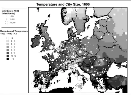
Figure 1 Temperature and City Size, 1600
Note: Map shows European year temperature averaged over 100 years, between 1500 and 1600. Data is taken from Luterbacher (2004). It shows location of cities in 1600 according to Bairoch (1988). Symbols are proportionate to city size.
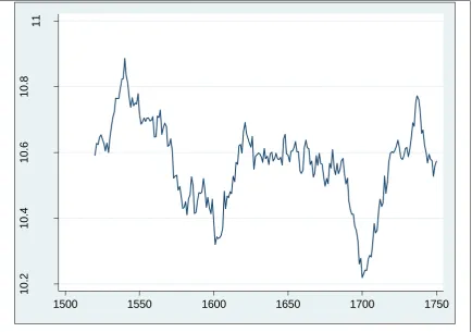
27 Figure 2 European annual mean temperature, 20 year moving average
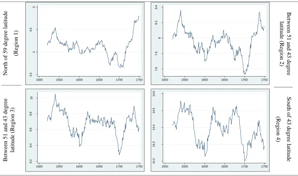
Figure 3 shows variation in mean temperature over time for different parts of Europe: north of 59 degree latitude, between 51 and 59 degree latitude, between 43 and 51 degree latitude, and south of 43 degree latitude. The figures show that temperature changed differently over time in these different areas. In the northernmost area of Europe (north of 59 degree latitude, including Scotland, Scandinavia, and the Baltic states) the cooling trend is almost uninterrupted, with only a short warm period around 1650 during which temperatures increase slightly. In the area between 51 and 59 degree latitude (Ireland and Great Britain, the Netherlands, north Germany and Poland) a temperature decrease of more than 0.6 degree Celsius between 1550 and 1600 is followed by 50 years of temperature during which temperatures increase by less than 0.4 degree Celsius. Between 43 and 51 degree latitude (France, the Alpines region, Austria, the Czech Republic and Slovakia) the cooling trend after 1550 is completely interrupted by a relatively warm and stable period of close to 100 years after 1600. In southern Europe (south of 43 degree latitude, including Spain, Italy and Greece) a short
1
0
.2
1
0
.4
1
0
.6
1
0
.8
11
T
emp
era
tu
re
(
°C
)
28 period of cooler temperatures after 1550 is completely compensated for by the following increase in temperature.
Table 1 Summary Statistics
Temperature in °C
Year All Region 1 Region 2 Region 3 Region 4
1600 10.6 4.2 8 9.72 14.41
1700 10.51 3.95 7.84 9.62 14.4
1750 10.6 4.46 8.1 9.71 14.33
City Size (number of inhabitants)
Year All Region 1 Region 2 Region 3 Region 4
1600 5440 1600 4600 5507 6251
1700 6500 3700 6836 6722 6033
1750 8258 9167 9134 8338 7365
Note: Regions 1 to 4 are defined as in Figure 3. Region 1 includes all cities north of 59 degree
29
Figure 3 European annual mean temperature as 20 years moving averages, according to latitude
Note: The top left graph presents annual mean temperature for the area north of 59 degree latitude. Countries in this area include Scotland, Scandinavian countries, and the Baltic states (Region 1). The top right graph presents annual mean temperature for the area between 51 and 59 degree latitude. Countries in this area include Ireland, Great Britain, the Netherlands, Belgium, northern Germany and Poland. The bottom left graph presents annual mean temperature for the area between 51 and 43 degree latitude. The area includes France, Switzerland, Austria, the Czech Republic, Slovakia, and Rumania. The bottom right graph presents data for the area south of 43 degree latitude including Spain, Italy and Greece.
3 .5 4 4 .5 5 T emp era tu re ( °C )
1500 1550 1600 1650 1700 1750
7 .6 7 .8 8 8 .2 8 .4 T emp era tu re ( °C )
1500 1550 1600 1650 1700 1750
9 .2 9 .4 9 .6 9 .8 10 T emp era tu re ( °C )
1500 1550 1600 1650 1700 1750
1 4 .2 1 4 .3 1 4 .4 1 4 .5 1 4 .6 T emp era tu re ( °C )
1500 1550 1600 1650 1700 1750
Nor
th of 59 de
gr ee latit u de (Re gion 1) B etwe
en 51 a
nd 43 d
egr ee latit ude ( R egion 2) B etwe
en 51 a
nd 43 d
egr ee lat it ude ( R egion 3) S
outh of 43
30 To investigate heterogeneity in the effect of temperature on city size I divide the sample according to climate groups (see Table 2). I define five climate groups based on the Geiger climate classification for Europe. I use data on the extent of Köppen-Geiger’s climate zones from Peel et al. (2007). The Köppen-Geiger climate classification divides the world into five major climate groups, denoted by the capital letters A to E. These climate groups are defined by temperature with A representing the warmest and E the coldest areas. An exception is climate group B whose defining characteristic is aridity. Subtypes of the groups are defined based on temperature and precipitation. In this chapter, I subdivide the sample into five climate groups. The climate group ‘arid hot climate’ represents Köppen-Geiger’s climate group B. The climate groups ‘temperate hot climate’ and ‘temperate warm climate’ represent Köppen-Geiger’s climate group C. The climate group ‘temperate hot climate’ represents a subgroup of Köppen-Geiger’s climate group C: temperate climate with hot summers. The climate group ‘temperate warm climate’ represents another subgroup of Köppen-Geiger’s climate group C: temperate climate with warm summers. The climate groups ‘moderately cold climate’ and ‘cold and alpine climate’ represent the Köppen-Geiger’s climate groups D and E. The climate group ‘moderately cold climate’ represents a subgroup of Köppen-Geiger’s climate group D: cold climate with hot or warm summers. The climate group ‘cold and alpine climate’ represents a subgroup of Köppen-Geiger’s climate group D and climate group E: cold climate with cold summers and Alpine climate.
Table 2 Climate Groups & Corresponding Koeppen-Geiger Climate Groups
Climate group KG Climate
Group KG Climate Subgroups
N° of Observations
Arid climate
Arid hot steppe 1 B Arid Arid cold steppe 140
Arid cold desert 2 Temperate Hot
Climate
C Temperate
Temperate climate with hot
dry summer 396
Temperate climate with hot
summer 152
Temperate Warm
31
Temperate climate with
warm summer 758 Moderately Cold
Climate
D Cold
Cold climate with hot
summer 26
Cold climate with warm
summer 491
Cold and Alpine
Climate E Polar
Cold climate with cold
summer 47
Polar Tundra 20
1.4.
Empirical Strategy
I use the panel data set for 2120 European cities to test whether temperature changes during the Little Ice Age, between 1500 and 1750, have affected city size. In the baseline specification, I include city fixed effects and year fixed effects. I further include various control variables. Each control variable is interacted with a full set of time period indicator variables.
(1) City Sizeit = β + γMean Temperatureit + yt + ii + cit + εict
City Size is the size of city i in time period t. MeanTemperatureit is mean year
temperature in city i, and time period t over the past 100 years (for the years 1600 and 1700) and past 50 years (for the year 1750, see also previous section for more detail). ii
are a full set of city fixed effects. The city fixed effects control for time-invariant city characteristics, e.g. distance to the sea and to waterways, permanent climatic or soil characteristics that may affect a city's access to trade or its agricultural productivity. yt
are a full set of year fixed effects that control for variation in temperature and in city size over time that is common to all cities in the data set. cit are a number of control
variables, each interacted with indicators for each time period. They will be described in more detail when introduced into the equation. εit is the error term. Standard errors
are clustered at the city level.
32 specification estimates the effect of temperature on city size based on variation in both variables within each city conditional on year fixed effects and on control variables interacted with time period indicators. The identification relies on the assumption that temperature changes are not correlated with other determinants of city size besides those that are controlled for.
1.5.
Baseline Results
1.5.1.
Basic Results and Geographic Controls
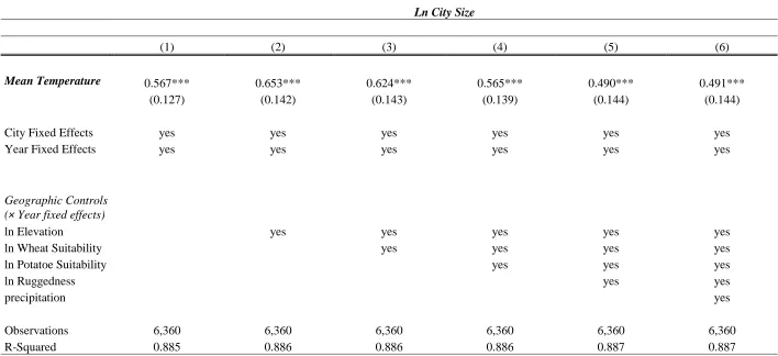
Table 3 shows baseline results. The table reports results for five different specifications. The first specification in column 1 estimates the effect of mean temperature on city size including city fixed effects and year fixed effects. The relationship is positive and significant at the 1% level. This indicates that temperature decreases during the Little Ice Age had a negative effect on city size which is consistent with historical evidence on the negative economic effects of the Little Ice Age. While current climate change is concerned about temperature increases above the temperature optimum, temperatures during the Little Ice Age dropped below the optimal temperature for European agriculture. Actually, climate researchers have predicted that Northern European agriculture - but only in the short-term and only for very small increases - might benefit from mild temperature increases due to its relatively cold climate (European Environmental Agency 2012: 158).
33
Table 3 The Effect of Temperature on City Size - Baseline Estimates and Geographic Controls
Ln City Size
(1) (2) (3) (4) (5) (6)
Mean Temperature 0.567*** 0.653*** 0.624*** 0.565*** 0.490*** 0.491***
(0.127) (0.142) (0.143) (0.139) (0.144) (0.144)
City Fixed Effects yes yes yes yes yes yes
Year Fixed Effects yes yes yes yes yes yes
Geographic Controls (× Year fixed effects)
ln Elevation yes yes yes yes yes
ln Wheat Suitability yes yes yes yes
ln Potatoe Suitability yes yes yes
ln Ruggedness yes yes
precipitation yes
Observations 6,360 6,360 6,360 6,360 6,360 6,360
R-Squared 0.885 0.886 0.886 0.886 0.887 0.887
34
1.5.2.
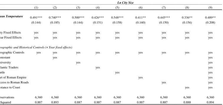
Controlling for Historical Determinants of Economic Growth
Results thus far show that temperature decreases of the Little Ice Age have had a negative effect on city size. This result is consistent with historical evidence on the negative effects of the Little Ice Age on economic conditions. In addition, I have controlled for a set of geographical variables that may have been correlated with both city size and temperature changes, each variable interacted with time indicator variables.
Yet, economic and urban growth has been uneven across Europe with especially high growth in Northwestern Europe. This pattern has been called by historians the Little Divergence. A number of factors have been held accountable for this divergence, e.g. the overseas trade expansion of the Atlantic powers and human capital accumulation. If temperature changes were correlated with these historical factors the estimated effect of temperature and city size would be biased. In the following, I therefore directly control for historical factors that have been identified as drivers of disparity in urban growth within Early Modern Europe.
Acemoglu, Johnson, and Robinson (2005) show that the overseas trade expansion of Western European countries had a positive effect on economic growth. I add an indicator for Atlantic traders, i.e. Great Britain, the Netherlands, Belgium, France, Spain, and Portugal.
As an additional measure for a country's natural openness for overseas trade I include an indicator variable for all cities located within 10 km of the coast.
Van Zanden (2009: 12) emphasises, among other factors, the importance of human capital accumulation for economic growth in Early Modern Europe. In the same vein, Cantoni and Yuchtman (2013) argue that the establishment of universities increased the number of people trained in law. This had a positive effect on economic activities in medieval Europe as it decreased the uncertainty of trade and. I include an indicator variable for cities that were university cities in 1500.
35 denomination was a highly political act. Rulers distanced themselves from the influence of the Roman Catholic Church that rejected, among other things, the newly developing ideas on scientific research (e.g. Merriman, 2010). As Protestantism may have affected economic development and hence city growth in these various ways I include indicator variables that are 1 if a city was majority Lutheran, Calvinist, Anglican, or Catholic in 1600.
Several studies identify war as an important factor in the development of Europe, e.g. through its effect on state-building (Tilly, 1990). Recently, Dincecco et al. (2013) argue that exposure to military conflict had a direct effect on urban growth as it induced people to seek protection from violence within city walls. I add a variable that measure the distance to the nearest battleground during the time period.
In column 6 of Table 4, I add an indicator variable that is 1 for all cities that were part of the Roman empire. In column 7 of table 3, I add an indicator variable for all cities that were located within one kilometer of a Roman road.
36
Table 4 Robustness Additional Historical Control Variables Ln City Size
(1) (2) (3) (4) (5) (6) (7) (8) (9)
Mean Temperature 0.491*** 0.740*** 0.500*** 0.426*** 0.548*** 0.411** 0.445*** 0.336** 0.489**
(0.144) (0.185) (0.144) (0.151) (0.158) (0.160) (0.150) (0.156) (0.208)
City Fixed Effects yes yes yes yes yes yes yes yes yes
Year Fixed Effects yes yes yes yes yes yes yes yes yes
Geographic and Historical Controls (× Year fixed effects)
Geographic Controls yes yes yes yes yes yes yes yes yes
Protestant yes yes
University yes yes
Atlantic Traders yes yes
Battle yes yes
Part of Roman Empire yes yes
Access to Roman Roads yes yes
Distance to Coast yes yes
Observations 6,360 6,360 6,360 6,360 6,360 6,360 6,360 6,360 6,360 R-Squared 0.887 0.893 0.887 0.887 0.887 0.887 0.887 0.888 0.894
Robust standard errors in parentheses, clustered at city level
37
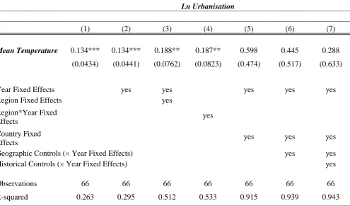
1.5.3.
The Effect of Temperature on Urbanisation
So far, city size has been used as an indicator of economic growth. In this section, I introduce urbanisationan as an alternative indicator of economic growth. In the absence of a direct measure, it has been widely used as a measure of historical per capita GDP by a number of studies (e.g. DeLong and Shleifer, 1993; Acemoglu, Johnson, and Robinson, 2002, 2005) and it has been shown that urbanisation has been strongly correlated with economic growth (e.g. Acemoglu, Johnson, and Robinson, 2002).
(2) Urbanisationct = β + γMean Temperaturect + yt + cc + gcct + hcct + εct
To estimate the effect of mean temperature on urbanisation I regress urbanisation in country c in time period t on a country’s mean temperature, year fixed effects, country fixed effects, and the previously introduced geographic and historical controls, each of them interacted with time period indicator variables.
Urbanisation is defined at the country level as the number of inhabitants living in cities divided by the total population. Countries are defined as in McEvedy and Jones (1978). The measure of urbanisation is available for 22 European countries and three time periods. Table 5 reports results from seven specifications. The first specification does not include controls. Each of the following specifications introduces one or more new controls. Specification (2) introduces year fixed effects in, specification (3) region fixed effects. Region times year fixed effects are included in specification (4) and country fixed effects in specification (5). Finally, the geographic and historical control variables as introduced previously in Table 3 and Table 4 are included in specifications (6) and (7).
38 variation used for estimation is much reduced. One might be concerned that the insignificant results in column (5) to (6) signify that the country fixed effect, hence country-wide institutional, economic or political factors – had been driving results. In this case, however, we would have expected to see a drop in the size of the coefficient and not only reduced statistical significance. It is reassuring that the size of the coefficients remains positive and relatively large.
Table 5 The Effect of Temperature on Urbanisation
Ln Urbanisation
(1) (2) (3) (4) (5) (6) (7)
Mean Temperature 0.134*** 0.134*** 0.188** 0.187** 0.598 0.445 0.288
(0.0434) (0.0441) (0.0762) (0.0823) (0.474) (0.517) (0.633)
Year Fixed Effects yes yes yes yes yes
Region Fixed Effects yes Region*Year Fixed
Effects yes
Country Fixed
Effects yes yes yes
Geographic Controls (× Year Fixed Effects) yes yes Historical Controls (× Year Fixed Effects) yes
Observations 66 66 66 66 66 66 66
R-squared 0.263 0.295 0.512 0.533 0.915 0.939 0.943
Robust standard errors in parentheses, clustered at country level
*** p<0.01, ** p<0.05, * p<0.1
1.6.
Robustness
1.6.1.
Alternative Samples
39 of low temperatures in Europe during the Little Ice Age. In Table 6, I test the robustness of these results to the exclusion of potential outliers. Columns 1 and 2 show the result of the baseline specification (1) with year fixed effects and with country times year fixed effects. Columns 3 to 10 explore whether the results are robust to the exclusion of potential outliers to test whether results are driven by a small number of especially fast growing cities. Each time I provide estimates for two specifications, one including city fixed effects and year fixed effects, the other including city fixed effects and country times year fixed effects.
In the early modern period, capital cities have grown particularly fast. In non-democratic societies rulers were free to invest a disproportionate share of tax income into the capital, e.g. into infrastructure project or the state bureaucracy. In columns 3 and 4, I exclude capital cities from the sample. Coefficients remain largely unchanged. Port cities have also grown especially fast because of their access to long distance trade. In columns 5 and 6, I exclude all potential port cities from the sample. Potential port cities are defined as cities that are located within 10 km of the Atlantic Ocean, Mediterranean Sea, North Sea, or Baltic Sea. Coefficients increase by 0.10 and 0.19 and increase in significance.
De Vries (1984: 140, see Table 7) provides a list of 34 cities that have been exceptionally successful because they were European capital cities, port cities or because they carried out industrial, commercial or administrative functions. In columns 7 and 8, I show that coefficient estimates decrease 0.03 and 0.02 and remain significant when excluding this group of cities.
40
Log CITY SIZE
Entire Sample
excl. capitals
excl. port cities
excl. successful cities
excl. Atlantic traders (1) (2) (3) (4) (5) (6) (7) (8) (9) (10)
Mean Temperature 0.579*** 0.540* 0.571*** 0.557* 0.680*** 0.733** 0.556*** 0.519* 0.534*** 0.981**
(0.127) (0.303) (0.128) (0.305) (0.160) (0.330) (0.129) (0.308) (0.157) (0.397) City Fixed Effects yes yes yes yes yes yes yes yes yes yes
Year Fixed Effects yes yes yes yes yes
Country*Year Fixed
Effects yes yes yes yes yes
Observations 6,345 6,345 6,291 6,291 5,037 5,037 6,246 6,246 3,711 3,711 R-Squared 0.885 0.899 0.881 0.895 0.878 0.897 0.880 0.895 0.892 0.907
Notes: Data are a panel of 2215 European cities. The left-hand-side variable is the natural log of number of city inhabitants. Mean temperature is year temperature averaged over the periods 1500 to 1600, 1600 to 1700, and 1700 to 1750. Country times Year fixed effects use country borders in 1600. The sample in columns 3 and 4 is restricted to cities that were not capital cities between 1600 and 1750. Regressions 5 and 6 include cities that are located more than 10 km from the sea. Regressions 7 and 8 exclude cities that were listed by de Vries (1984:140) as especially successful, fast growing cities between 1600 and 1750. Regression 8 includes cities that were not located in one of the countries identified in Acemoglu et al. (2005) as Atlantic traders: Portugal, Spain, France, England, and the Netherlands.
Robust standard errors in parentheses, clustered at city level. *** p<0.01, ** p<0.05, * p<0.1
41 Table 7 Fastest Growing Cities in Europe in 1600
Amsterdam Clermont-Ferrand Liege Nimes Berlin Copenhagen Liverpool Norwich London Cork Livorno Prague Madrid Dresden Lyon Rotterdam
Paris Dublin Malaga Stockholm Turin Glasgow Nancy Toulon Brest The Hague Nantes Versailles Bristol Leipzig Newcastle Vienna
Cadiz Kaliningrad
Note: The table contains a list of cities, especially capital cities, port cities, and cities that served as administrative or trade centres that were identified by de Vries (1984: 140) as especially successful, fast-growing cities in early modern Europe.
1.6.2.
Alternative Fixed Effects and Time Trends
In this section, I test whether the estimated effect of mean temperature on city size is robust to the inclusion of alternative spatial fixed effects and time trends at different levels. Column 1 of Table 8 shows a specification including city fixed effect and year fixed effects. In column 2, I introduce a linear time trend at the country level. In column 3, the country level time trend is replaced by country level fixed effects. In column 4, a country level time trend is added to the specification. Then, the country level fixed effects are replaced by period specific fixed effects in column 4. Finally, a time-period specific country time trend is added in column 5 and a city specific time trend in column 6. For the period specific country fixed effects, each city is assigned to the country that it was located in in each time period. If city X was part of country A in time period t but was part of country B in time period t+1, then country A is assigned to city X in time period t and country B is assigned in time period t+1. This takes into account changing country borders over the course of the period under study.
42 include city level time trends. For these specifications standard errors could not be estimated, possibly because the combination of city fixed effects, year fixed effects, period-specific country fixed effects and a city time trend is too demanding as the data contains three observations per city.
Table 8 Alternative Fixed Effects and Time Trends
Ln City Size
(1) (2) (3) (4) (5) (6) (7)
Mean Temperature
0.564*** 0.259** 0.526* 0.420 0.620*** 0.345*** 0.397 (0.127) (0.127) (0.299) n/a (0.125) (0.130) n/a
Fixed Effects
City FE yes yes yes yes yes yes yes
Year FE yes yes yes yes yes
Country in 1600
× Year FE yes yes
Period-Specific
Country FE yes yes yes
Linear Time Trend
Country in 1600 yes Period-Specific
Country yes
City yes yes
Observations 6,360 6,360 6,360 6,360 6,360 6,360 6,360 R-Squared 0.885 0.895 0.899 0.974 0.888 0.899 0.972
Robust standard errors in parentheses, clustered at city level *** p<0.01, ** p<0.05, * p<0.1
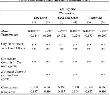
1.6.3.
Using Alternative Standard Errors
43 controls (column 2). Column 3 and 4 show the same two specifications when clustering at the grid cell level of the underlying temperature data set. Temperature data is provided by grid cell (see section 3 for more detail). Each city is assigned temperature data of the grid cell that the city is located in. Different cities can have been assigned the same temperature data if they are located in the same grid cell. All cities whose temperature data has been informed by the same observation in the temperature reconstruction dataset form a cluster. Finally, column 5 and show the two specifications using Conley standard errors. Conley standard errors assume spatial autocorrelation for cities located within 100 km from each other. Spatial autocorrelation is assumed to decrease with distance between cities and complete independence is assumed for cities located further than 100 km apart.
[image:43.595.134.521.364.696.2]
Table 9 Robustness Using Alternative Standard Errors
Ln City Size Clustered at…
City Level Grid Cell Level Conley SE
(1) (2) (3) (4) (5) (6)
Mean Temperature
0.487*** 0.483** 0.487*** 0.483** 0.487*** 0.483** (0.144) (0.208) (0.172) (0.224) (0.173) (0.200) City Fixed Effects yes yes yes yes yes yes Year Fixed Effects yes yes yes yes yes yes
Geographic Controls (× Year fixed effects)
yes yes yes yes yes yes
Historical Controls (× Year fixed effects)
yes yes yes
Observations 6,360 6,360 6,360 6,360 6,360 6,360 R-Squared 0.887 0.894 0.887 0.894 0.887 0.894 Robust standard errors in parentheses, clustered at different levels
44
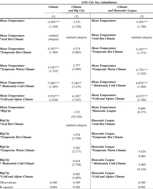
1.6.4.
The Effect of Temperature in Different Climate Zones
The 2007 report of the Intergovernmental Panel on Climate Change (IPCC, Parry et al., 2007) predicts that the effect of temperature change on agricultural productivity will be different in different climate zones. “In mid- to high-latitude regions [far from the equator], moderate warming benefits cereal crop and pasture yields, but even slight warming decreases yields in seasonally dry and tropical region,” (Parry et al., 2007: 38). Schlenker et al. (2009) find that increases in temperature up to a certain point lead to increases in yield. After reaching an optimum further increases lead to a steep decline in yield. In this section, I test whether the effect of temperature change on city size during the Little Ice Age is different for cities in different climate zones within Europe. Mean annual temperature varies significantly across Europe (see Figure 1 for mean annual temperature across Europe in 1600). The difference between the warmest and the coldest areas is more than 12 degrees. The question arises whether the effect of temperature on city size varies with initial climate.
For this purpose, I divide the sample into five subsamples based on the Köppen-Geiger climate zones for Europe (see section 1.3 for a detailed description). The five subsamples represent five climate groups: arid and hot climate, temperate hot climate, temperate warm climate, moderately cold climate, and cold, alpine climate (see Figure 4 for a map). The groups with arid, hot climate and cold, alpine climates are the smallest with 143 and 67 cities respectively. Arid, hot climate prevails in parts of Spain, and cold, alpine climate in parts of Scandinavia and Russia, and in the Alps. The groups with temperate, hot climate, temperate warm climate, and moderately cold climate comprise between 517 and 839 cities. Temperate, hot climate prevails in the area bordering on the Mediterranean Sea. Temperate warm climate prevails in large parts of north-western Europe, e.g. England, the Netherlands, and France, and in parts of Germany and Spain. Moderately cold climate prevails in large parts of Eastern Europe. To examine whether the effect of temperature depends on a location’s initial climate I divide the sample into five subsamples each containing all the cities within one climate zone. I split the sample according to climate groups and estimate specification (3).
45 Figure 4 European Climate Groups
Note: This map shows the distribution of climate groups across Europe. The definition of climate groups follows the Koeppen-Geiger definition (Peel et al., 2007). Arid hot climate corresponds to Koeppen-Geiger climate group B. Temperate hot climate corresponds to Koeppen-Geiger climate groups Csa and Cfa. Temperate warm climate corresponds to Geiger climate groups Csb and Cfb. Moderately cold climte corresponds to Koeppen-Geiger climate groups Dfa and Dfb, and Cold and alpine climate corresponds to Koeppen-Koeppen-Geiger climate groups Dfc and ET.
The coefficient of interest is γ, the estimated effect of temperature on city size. The specification also contains a full set of country times year fixed effects, cy, and a full set of city fixed effects, i. ε denotes an error term. The subscripts i, c, and t denote city, country and time period respectively.
47
Table 10 The Effect of Temperature in Different Climate Zones
LOG City Size (inhabitants)
Entire Sample Arid Hot Climate Temperate Hot
Climate
Temperate Warm Climate
Moderately Cold Climate
Cold and Alpine Climate
Latitude (°N) 46.63 39.01 40.72 49.12 50.63 49.18
Longitude (°E) 8.87 -2.05 10.6 9.97 20.38 12.48
Temperature (°C) 10.71 14.39 14.15 9.99 7.7 7.48
(1) (2) (3) (4) (5) (6)
Mean Temperature 0.540* -4.222*** -0.0485 -0.00134 1.011 1.367
(0.303) (1.120) (0.881) (0.532) (0.662) (1.550)
Country*Year Fixed
Effects yes yes yes yes yes yes
City Fixed Effects yes yes yes yes yes yes
Observations 6,345 429 1,644 2,517 1,551 201
R-squared 0.899 0.947 0.947 0.879 0.872 0.919
Note: Data are a panel of 2215 European cities. The left-hand-side variable is the natural log of number of city inhabitants. Mean temperature is year temperature averaged over the periods 1500 to 1600, 1600 to 1700, and 1700 to 1750. The definition of climate groups follows the Koeppen-Geiger definition (Peel et al. 2007). Arid hot climate corresponds to Koeppen-Geiger climate group B. Temperate hot climate corresponds to Koeppen-Geiger climate groups Csa and Cfa. Temperate warm climate corresponds to Koeppen-Geiger climate groups Csb and Cfb. Moderately cold climate corresponds to Koeppen-Geiger climate groups Dfa and Dfb, and Cold and alpine climate corresponds to Koeppen-Geiger climate groups Dfc and ET.
48
1.7.
The Role of Agricultural Productivity
1.7.1.
The Effect of Temperature on Wheat Prices
The results have shown that the effect of temperature on city size varies across climate zones. The question arises through which channel this effect occurs. Historians have argued that the Little Ice Age affected agricultural productivity. Fruit blossoming, haymaking and grape ripening were delayed because of cold weather (Behringer, 2010: 93). “Shortened growing seasons [during the Little Ice Age] led to reductions in agricultural productivity, especially in northern Europe,” (Aguado, 2007: 483). The overwhelming importance of agriculture for the economy at the time also makes it plausible that temperature may have affected city size through its effect on agricultural productivity. “The growth rates of agricultural outputs and productivity within each country were the primary determinants of overall growth rates in each [European] country,” (Dennison, 2010: 148). It is therefore plausible that a negative effect of disadvantageous weather conditions during the Little Ice Age on agricultural productivity may have translated into an effect on city