R E S E A R C H
Open Access
A modified exact smooth penalty function for
nonlinear constrained optimization
Liu Bingzhuang
*and Zhao Wenling
*Correspondence: [email protected] School of Science, Shandong University of Technology, Zibo, Shandong 255049, P.R. China
Abstract
In this paper, a modified simple penalty function is proposed for a constrained nonlinear programming problem by augmenting the dimension of the program with a variable that controls the weight of the penalty terms. This penalty function enjoys improved smoothness. Under mild conditions, it can be proved to be exact in the sense that local minimizers of the original constrained problem are precisely the local minimizers of the associated penalty problem.
MSC: 47H20; 35K55; 90C30
Keywords: constrained minimization; exact penalty function; nonlinear programming problem
1 Introduction
Merit function has always taken an important role in optimization problem. It is tradi-tionally constructed to solve nonlinear programs by augmenting the objective function or a corresponding Lagrange function some penalty or barrier terms with respect of the constraints. Then it can be optimized by some unconstrained or bounded constrained op-timization softwares or sequential quadratic programming (SQP) techniques. No matter what kind of techniques are involved, the merit function always depends on a small pa-rameterεor large parameterρ=ε–. Asε→, the minimizer of a merit function such as a barrier function or the quadratic penalty function, converges to a minimizer of the original problem. By using some exact penalty function such aslpenalty function (see
[, , –]), the minimizer of the corresponding penalty problem must be a minimizer of the original problem whenεis sufficiently small. There are some nonsmooth penalty functions for nonsmooth optimization problems, such as the exact penalty function using the distance function for the nonsmooth variational inequality problem in Hilbert spaces [] and the one in [].
The traditional exact penalty functions [] are always nonsmooth. When it is used as a merit function to accept a new iterate in an SQP method, it may cause the Maratos effect []. On the other hand, a traditional smooth penalty function like the quadratic penalty function cannot be an exact one. So we must compute a sequence of minimization sub-problem asε→. At that time, ill-conditioning may occur when the penalty parameter is too large or small, which also brings difficulty of computation. In [] and [], some kinds of augmented Lagrangian penalty functions have been proposed with improved exactness under strong conditions. In [], exact penalty functionsviaregularized gap function for variational inequalities have also been given. All these functions enjoy some smoothness,
but at the very beginning, to use this smoothness we need second-order or third-order derivative information of the problem function that is difficult to estimate in practice. Besides, all the above kinds of penalty functions (see [–, , ] for summary) may be unbounded below even when the constrained problem is bounded, which may make it difficult to locate a minimizer.
In the paper [], a new penalty function is proposed for the constrained optimization problem. By augmenting the dimension of the program with an additional variableεthat controls the weight of the penalty terms, this new penalty function enjoys properties of smoothness and exactness, and remains bounded below under reasonable conditions. Its important new idea is that the penalty function is considered as a function of variablex
and the additional variableεsimultaneously. Under proper assumptions, the minimizer (x*,ε
*) of the merit function satisfiesε*= , andx*is a minimizer of the original problem.
However, the penalty function given in [] is not smooth in a small neighborhood of (x*, ), where the minimizer of the original constrained problem lies. In this paper, we give
a penalty function which enjoys the properties of the penalty function given in [] and has improved smoothness.
The rest of this paper is organized as follows. In Section , a penalty function is in-troduced for a smooth nonlinear optimization problem with equality constraints and bounded constraints. The smoothness of this penalty function is discussed, as well as other properties, including being bounded below under mild assumptions. Section shows the exactness of our penalty function in the sense that under certain conditions, local mini-mizer of our penalty function has the form (x*,ε
*) withε*= andx*is a local minimizer
of the original problem, and a converse result holds.
Notation Throughout this paper, we use the Euclidean normx=x
k. The
subvec-tor ofxindexed by the indices inJis denoted byxJ. We denote sets of the form
[x,x] :=x∈Rn|{x≤x≤x},
where the lower boundx∈(R∪ {–∞})nand the upper boundx∈(R∪ {∞})nare vectors containing proper or infinite bounds on the components ofxand [x,x] is referred to an
n-dimensional box.
2 New penalty function
We consider the smooth nonlinear optimization problem with equality constraints and bound constraints:
(P) minf(x)
s.t. x∈[u,v], F(x) = , (.)
where [u,v] is a box innwith nonempty interior,f :D→ andF:D→ m are
con-tinuously differentiable in an open setDcontaining [u,v] andm<n. We fixw∈ mand
consider the equivalent problem:
(P)
minf(x)
s.t. Fj(x) =εγwj, j= , . . . ,m, x∈[u,v],ε= ,
(.)
Letε> be an upper bound of the parameterε. Then the corresponding penalty func-tionfσ onD×[,ε] for (P) is given as follows:
fσ(x,ε) = ⎧ ⎪ ⎨ ⎪ ⎩
f(x) ifε= (x,ε) = ,
f(x) +
εα (x,
ε) –q (x,ε)+σ ε
β ifε> , (x,ε) <q–,
+∞ otherwise
(.)
with the constraint violation measure
(x,ε) :=F(x) –εγw,
where, in addition, γ >α≥β≥ andq> , are all fixed numbers, σ> is a penalty parameter and · is a Euclidean norm, withx=√xTxfor any vectorx.
Obviously,ε= (x,ε) = if and only ifε= ,Fj(x) = ,j= , . . . ,m. The corresponding
penalty problem then reads
(Pσ)
minfσ(x,ε)
s.t. (x,ε)∈[u,v]×[,ε]. (.)
The main difference between (.) and the penalty function given in [] is that in (.), β(ε) =εβ, which does not have the property thatβ(ε)→+∞, asε→+.
It is easy to see thatfσ(x,ε) is continuously differentiable with respect to (x,ε) on
Dq:= (x,ε)∈D×(,ε]≤ (x,ε) <
q
.
2.1 Boundedness of the penalty function
IfF(x) = , (x,ε)∈Dq, then
fσ(x,ε) =f(x) +
εγ–αw
–qεγw+σ ε
β≥f
σ(x, ) =f(x). (.)
Therefore,fσ(x,ε) is bounded below on the set
D=x∈[u,v]|F(x)≤q–/+εγw,
wheneverf(x) is bounded below on the setD. This is a reasonable condition since it usu-ally holds whenf is bounded below on the feasible set,εis small enough, andqis large enough.
The denominator –q (x,ε) is included since it forces the level sets offσ to remain in the set{(x,ε)∈ n+| (x,ε) <q–}, hence in some sense does not go far away from the
feasible set of (P).
Now we see a simple example:
minx
s.t. x– = ,
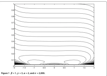
Figure 1 β= 1,γ= 3,α= 2, andσ= 2,000.
It has a bounded feasible domain, a global minimizer atx*= – withf(x*) = –, and a local
minimizerx= . The traditional quadratic penalty function for this problem
P(x) =x+ ε
x– ,
is unbounded below for all penalty parametersε> since,e.g., p(x)→–∞forx= –s,
s→+∞. It is also the case for traditional penalty functions, including multiplier penalty functions that use an additional term +λ(x– ). On the other hand, our new penalty
func-tion is bounded below. Setw= , it reads
fσ(x,ε) = ⎧ ⎪ ⎨ ⎪ ⎩
x ifε=r= ,
x+
εα r
–qr +σ εβ ifε> ,|r|<q–/,
+∞ otherwise,
wherer= +εγ –x. Sincef
σ(x,ε) = +∞, if|x| ≥
q–/+ +εγ, it is obvious that our penalty function is bounded below. See Figure for the display of the contour of the penalty function on this example.
3 Exactness of the penalty function
In this section, we show that our penalty function is exact in the sense that under certain conditions, local minimizer of our penalty function has the form (x*,ε
*) in whichε*=
andx*is a local minimizer of the original problem and a converse proposition holds.
Firstly, recall the Mangasarian-Fromovitz condition. We say that the Mangasarian-Fromovitz condition (see []) for Problem (P) holds at x∈[u,v]if F(x)has full rank and there is a vector p∈ nwith F(x)p= and
pi
> if xi=ui,
< if xi=vi.
Theorem . Assume that the set Ddefined in Section is bounded, and the Mangasarian-Fromovitz condition holds at each x∈D. Letγ >α≥β≥in (Pσ). Ifσ is sufficiently
large, then there is no Kuhn-Tucker point(x,ε)of (Pσ) withε> .
Proof Let the Lagrangian function of (Pσ) forσ> be
L(x,ε,y,z) =fσ(x,ε) +
n
i=
yi(ui–xi) + n
i=
zi(xi–vi) +yn+(–ε) +zn+(ε–ε),
whereyi,zi∈ ,i= , . . . ,n+ are the Lagrangian multipliers. If (x,ε) is a Kuhn-Tucker
point of (Pσ) withε> , then there exist vectorsy,z∈ n+such that
∇(x,ε)L(x,ε,y,z) = ,
ui–xi≤, xi–vi≤, i= , . . . ,n,
–ε< , ε–ε≤,
yi(ui–xi) = , zi(vi–xi) = , zn+(ε–ε) = , yn+ε= ,
then
∇(x,ε)fσ(x,ε) =y–z,
and
inf(yi,xi–ui) =inf(zi,vi–xi) = , i= , . . . ,n,
yn+=inf(zn+,ε–ε) = ,
where∇(x,ε)fσ(x,ε) is the gradient offσwith respect to (x,ε). The assertion of the theorem
is proved by contradiction.
Assume that there exists a sequence{(xk,εk,σk)}withεk> for allk,σk→+∞ask→
∞, where (xk,ε
k) is a Kuhn-Tucker point of (Pσk). We use the abbreviation k:= (x k,ε
k).
The pointxksatisfies
Fxk≤ /k +εkγw ≤q–/+εγw,
hence,xk∈D={x∈[u,v]|F(x) ≤q–/+εγw}. SinceDis closed and bounded, we may restrict ourselves to a subsequence if necessary and assume that
lim
k→∞εk=ε*∈[,ε] and klim→∞x
k=x*∈D.
The condition∂ε∂fσ(xk,εk)≤ yields
αq k+ (γ–α)εkγw+ (α–γ)εkγ
m
j= Fj
xkwj
+βεkα+β( –q k)σk≤α m
j=
with equality in the caseεk=ε. Whenσk→ ∞and becauseα
m
j=Fj(xk) - the right side
of (.) is a finite number, we have
lim
k→∞εk=ε*= or klim→∞
xk,ε k
= *=q–, (.)
where *= (x*,ε
*). On the other side, the derivative the penalty functionfσ with respect toxis given as
∂ ∂xi
fσ
xk,εk
= ∂
∂xi
fxk+ εα
k
∂ ∂xi (x
k,ε k)
–q (xk,ε k)
+ εα
k
q (xk,ε k)∂∂x
i (x k,ε
k)
( –q (xk,ε k))
= ∂
∂xi
fxk+ εα
k
∂ ∂xi (x
k,ε k)
( –q (xk,ε k))
⎧ ⎪ ⎨ ⎪ ⎩
≥ ifxki =ui,
= ifui<xki <vi,
≤ ifxk i =vi
(.)
(.) is equivalent to
εαk –q xk,εk
∂
∂xi
fxk+ ∂ ∂xi
xk,εk
=εkα –q xk,εk
∂
∂xi
fxk+ FxkTFxk–εkγwi
⎧ ⎪ ⎨ ⎪ ⎩
≥ ifxk i =ui,
= ifui<xki <vi,
≤ ifxki =vi.
(.)
Letk→+∞, sinceε*= or *=q–, we have
Fx*TFx*–εγ*wi
⎧ ⎪ ⎨ ⎪ ⎩
≥ ifx* i=ui,
= ifui<x*i<vi,
≤ ifx* i=vi.
(.)
Becausex*∈D, thus Mangasarian-Fromovitz condition holds atx*and there exists some
vectorp∈ nsuch thatF(x*)p= , wherepsatisfies (.). LetI
:={i|x*i=ui},I:={i|x*i= vi}and *:=F(x*) –ε
γ
*w. Then by (.), we have
=Fx*pT *= i∈I
pi
Fx*T * i+
i∈I
pi
Fx*T *
i. (.)
(.) and the Mangasarian-Fromovitz condition (.) imply (F(x*)T *)
i= fori∈I∪I.
Thus,F(x*)T *= . Now the fact thatF(x*) has full rank yields *= ,i.e.,
Fx*–εγ*w= ,
and by *=lim
k→∞(F(xk) –ε
γ
kw) = , it follows that
lim k→∞
xk,εk
= lim
k→∞F
By (.), we obtain
lim
k→∞εk=ε*= .
Thus,limk→∞F(xk) =F(x*) = .
Furthermore, by (.), it holds that
q
εαk+β
xk,ε k
+
γ α–
εαk+β–γw
+
–γ
α
εkγ–(α+β)
m
i= Fi
xkwi
+β α
–q xk,εk
σk≤
m
i=Fi(xk)
εkα+β .
Letk→ ∞, the last term on the left-hand side tend to +∞. Thus, the vectorsyk= F(xk)
ε
α+β
k
satisfiesyk →+∞. The vectorszk= yk
ykhave norm , and (.) implies that the numbers
μki (i= , . . . ,n), defined by
μki =
yk
∂ ∂xi
fxk+
yk
εαk( –q (xk,ε
k))
FxkTF(xk) –εkγw
i
=
yk
∂ ∂xi
fxk+ ε
α–β
k ( –q (xk,εk))
FxkT
zk–ε γ–α+β
k w yk i , satisfy
μki ⎧ ⎪ ⎨ ⎪ ⎩
≥ ifxk i =ui,
= ifui<xki <vi,
≤ ifxki =vi.
If we pick a convergent subsequenceznk with the limitz*and pass to the limit we obtain
Fx*z*i
⎧ ⎪ ⎨ ⎪ ⎩
≥ ifx* i=ui,
= ifui<x*i<vi,
≤ ifx* i=vi.
Now similarly as above, it yieldsz*= , which is a contradiction withz*= . Thus such a
sequence{(xk,ε
k,σk)}cannot exist, and for sufficiently largeσ> , all Kuhn-Tucker points
of (Pσ) are of the form (x, ).
Theorem . Assume that(x*,ε*)is a local minimizer of minimizer of (Pσ) with finite
fσ(x*,ε*), whereσ> is sufficiently large. If the hypotheses of Theorem . are fulfilled, then x*is a local minimizer of (P).
Proof Now let (x*,ε
*) be a local minimizer of (Pσ) with finitefσ(x*,ε*) andσ> is
implies thatF(x*) = , and by (.) there is a neighborhoodN(x*) ofx*wheref(x)≥f(x*)
for feasiblex. Therefore,x*is a local minimizer of (P).
We now show a converse result of Theorem ., which will use the following lemmas.
Lemma . Suppose F(x*) = , and F(x*)has full rank. Then there exist a neighborhood N(x*)of x* and a constant κ> such that for each x∈N(x*), and each subset J of
{, , . . . ,m}, there exists a vector y=y(x)∈N(x*)with Fi(y) = , for i∈J and Fi(y) =Fi(x), i∈K={, , . . . ,m} \J, such that
x–y ≤κFJ(x).
Proof SinceF(x*) = andF(x*) has full rank, there exists a matrixB∈ (n–m)×nsuch that the augmented matrixF(x*)
B
is nonsingular. By the continuity ofF(·) atx*, there exists
a neighborhoodN(x*)⊂Dofx*such that
F(x) B
is nonsingular, for anyx∈N(x*). Take
forAthe closed convex hull of{F(x)|x∈N(x*)}, then for allA∈A, the matrix
A
B
is nonsingular. We now show that for anyx,y∈N(x*), there exists a matrixA∈Asuch that
F(x) –F(y) =A(x–y). (.)
In fact, givenx,y∈N(x*), it follows from the mean value theorem that
F(x) –F(y) =
Fy+s(x–y)(x–y)ds
=Ax,y(x–y),
whereAx,y=
F(y+s(x–y))ds∈A, so (.) holds. Set the mappingH(z) :=
F(z)
B(z–x*)
, for
z∈N(x*). By the proof in [, Theorem .], we have that there exists a neighborhood N(x*)⊂N(x*) ofx*such that for eachx∈N(x*), and each subsetJof{, , . . . ,m}, there
exists a vectory=y(x)∈N(x*) with
H(y) =
F(y)
B(y–x*)
=
⎛ ⎜ ⎝
FK(x) B(x–x*)
⎞ ⎟ ⎠,
soFi(y) = , fori∈JandFi(y) =Fi(x),i∈K.
Forx,y∈N(x*), we have
H(x) –H(y) =
A B
(x–y),
for someA∈A. On the other side, we have
Therefore, combining (.) with (.), we have
x–y ≤
A B
–
FJ(x)≤κFJ(x),
where
κ:=
Asup∈A
A B
–
< +∞,
and this complete the proof.
Lemma . Assume that x*is a local minimizer of problem (.) with u
i≤x*i≤vi, i∈
{, . . . ,p}, where m≤p≤n. Suppose that F(x*)has full rank. Then there exists a constant
κ> such that
f(x)≥fx*–κF(x), for all x∈N
x*,
where N(x*)is defined in Lemma ..
Proof From Lemma ., letN(x*) andκbe the one in Lemma .. Letx∈N(x*), then
by Lemma . withJ={, . . . ,m}, there exists any=y(x) withF(y) = andyi=x*i, i= m+ , . . . ,nsuch that
x–y ≤κF(x). (.)
Soyis a feasible point of problem (.), andf(y)≥f(x*). Sincef is continuously
differen-tiable, for anyx,y∈N(x*), there exists a vectorξ∈ nsuch that
f(x) –f(y) =∇f(ξ)T(x–y),
whereξ lies in the segment betweenxandy. SetL:=supz∈N(x*)∇f(z), we have f(x) –f(y)≤∇f(ξ)x–y
≤Lx–y
≤LκF(x),
where the last inequality holds from (.). Letκ=Lκ, then
f(x) =f(x) –f(y) +f(y)≥fx*–κF(x),
Theorem . If x*is a local minimizer of problem (P) with u
i≤x*i≤vi, i∈ {, . . . ,p}, where m≤p≤n, and F(x*)has full rank, then for sufficiently largeσ> , there are a neighbor-hood N(x*)of x*and aε∈(,ε]such that
fσ(x,ε) >fσ
x*, =fx*, for all(x,ε)∈Nx*×(,ε].
In particular,(x*, )is a local minimizer of f
σ.
Proof LetN(x*)⊂N(x*) is a neighborhood ofx*such that sup
x∈N(x*)
fx*–f(x)< , (.)
whereN(x*) is defined in Lemma ..
For (x,ε)∈N(x*)×(,ε], whereε∈(,ε] andε≤, we distinguish two cases. Case . (x,ε) =F(x) –εγw≥εα. For this case, we have
fσ(x,ε)≥f(x) + +σ εβ
≥fx*+σ εβ >fx*=fσ
x*, ,
where the second inequality is by (.).
Case . (x,ε) <εα. ThenF(x) ≤ +εγw ≤εα +εγw, and
fσ(x,ε)≥f(x) +σ εβ
≥fx*–κF(x)+σ εβ
≥fx*–κ
εα +εγw+σ εβ
≥fx*+σ–κ
+εγ–αwεα. (.)
The last inequality holds sinceβ≤α. Letσ>κ( +εγ–
α
)w, we get
fσ(x,ε)≥f
x*=fσ
x*, .
From Case and Case , we obtain the conclusion.
4 Conclusion remarks
In this paper, a modified exact penalty function for equality constrained nonlinear pro-gramming problem is constructed by augmenting a new variable that controls the con-straint violence. This function enjoys smoothness, and with very mild conditions it is proved to be an exact penalty function.
properties to nonsmooth optimization problems, just as that has been done in [–]. That will be our future research direction.
Competing interests
The authors declare that they have no competing interests.
Authors’ contributions
All authors read and approved the final manuscript.
Acknowledgements
The authors wish to thank the anonymous referees for their endeavors and valuable comments. The authors would also like to thank Professor Zhang Liansheng for some very helpful comments on a preliminary version of this paper. This research was supported by the National Natural Science Foundation of China under Grants 10971118, 11101248, Natural Science Foundation of Shandong Province under Grants ZR2012AM016, and the foundation 4041-409012 of Shandong University of Technology.
Received: 13 February 2012 Accepted: 26 July 2012 Published: 6 August 2012 References
1. Antczak, T: Exact penalty functions method for mathematical programming problems involving invex functions. Eur. J. Oper. Res.198, 29-36 (2009)
2. Bazaraa, MS, Sherali, HD, Shetty, CM: Nonlinear Optimization Theory and Algorithms, 2nd edn. Wiley, New York (1993) 3. Bertsekas, DP: Constrained Optimization and Lagrange Multiplier Methods. Academic Press, New York (1982) 4. Boukari, D, Fiacco, AV: Survey of penalty, exact-penalty and multiplier methods from 1968 to 1993. Optimization32,
301-334 (1995)
5. Clarke, FH: Optimization and Nonsmooth Analysis. Wiley-Interscience, New York (1983)
6. Di Pillo, G: Exact penalty methods. In: Spedicato, E (ed.) Algorithms for Continuous Optimization, pp. 209-253. Kluwer Academic, Dordrecht (1994)
7. Fletcher, R: Practical Methods of Optimization, 2nd edn. Wiley, New York (1987)
8. Han, SP, Mangasarian, OL: Exact penalty functions in nonlinear programming. Math. Program.17, 251-269 (1979) 9. Hoheisel, T, Kanzow, C, Outrata, J: Exact penalty results for mathematical programs with vanishing constraints.
Nonlinear Anal.72, 2514-2526 (2010)
10. Huyer, W, Neumaier, A: A new exact penalty function. SIAM J. Optim.13, 1141-1158 (2003)
11. Li, W, Peng, J: Exact penalty functions for constrained minimization problems via regularized gap function for variational inequality. J. Glob. Optim.37, 85-94 (2007)
12. Mangasarian, OL, Fromovitz, S: The Fritz John necessary optimality conditions in the presence of equality and inequality constraints. J. Math. Anal. Appl.17, 37-47 (1967)
13. Maratos, N: Exact penalty function algorithms for finite dimensional and control optimization problems. PhD thesis, University of London (1978)
14. Mordukhovich, BS: Variations Analysis and Generalized Differentiation, I: Basic Theory. Grundlehren Series (Fundamental Principles of Mathematical Sciences), vol. 330. Springer, Berlin (2006)
15. Mordukhovich, BS: Variations Analysis and Generalized Differentiation, II: Applications. Grundlehren Series (Fundamental Principles of Mathematical Sciences), vol. 331. Springer, Berlin (2006)
16. Nocedal, J, Wright, SJ: Numerical Optimization. Springer, New York (1999)
17. Soleimani-damaneh, M: The gap function for optimization problems in Banach spaces. Nonlinear Anal.69, 716-723 (2008)
18. Soleimani-damaneh, M: Penalization for variational inequalities. Appl. Math. Lett.22, 347-350 (2009)
19. Soleimani-damaneh, M: Nonsmooth optimization using Mordukhovich’s subdifferential. SIAM J. Control Optim.48, 3403-3432 (2010)
20. Zangwill, WI: Nonlinear programming via penalty function. Manag. Sci.13, 344-358 (1967)
21. Zaslavski, AJ: A sufficient condition for exact penalty in constrained optimization. SIAM J. Optim.16, 250-262 (2005) 22. Zaslavski, AJ: Stability of exact penalty for nonconvex inequality-constrained minimization problems. Taiwan. J. Math.
14, 1-19 (2010)
doi:10.1186/1029-242X-2012-173