North American Integration and the Location of Foreign Direct Investment

(1)

Munich Personal RePEc Archive

North American Integration and the

Location of Foreign Direct Investment

Tekin-Koru, Ayca and Waldkirch, Andreas

Colby College

July 2007

(2)

North American Integration and the Location of

Foreign Direct Investment

∗

Ayça Tekin-Koru

†

_{and Andreas Waldkirch}

‡

July 2007

Abstract

We investigate how the North American Free Trade Agreement (NAFTA) has altered the pattern of foreign direct investment (FDI) in North America. The theoretical analysis suggests that NAFTA affects the incentives of U.S. and non-U.S.firms locating in Mexico differently and may lead to investment diversion from the U.S. Combining U.S. and Mexican FDI data and using a difference-in-differences estimator, wefind that U.S. FDI in Mexico has increased since the inception of NAFTA in a manner that cannot be explained entirely by the usual FDI determinants. Other countries have been using Mexico as an export platform since before NAFTA with no discernible positive effect from the agreement. We find little evidence that inward U.S. FDI has been diverted. The results are robust to a number of different model and econometric specifications as well as the skill data used.

Keywords: Foreign Direct Investment, Multinationals, Export Platform, NAFTA.

JEL Classiﬁcation: F15, F21, F23.

∗_{We would like to thank seminar participants at the University of Oregon, Bilkent University, the Midwest}

International Economics Conference at Vanderbilt University, the Western Economic Association International Conference in San Francisco and the Empirical Investigations in International Trade Conference at Purdue Uni-versity for useful comments and discussion.

†

Department of Economics, Oregon State University, 303 Ballard Hall, Corvallis, OR 97331. E-mail: [email protected]

‡

(3)

1 Introduction

A salient feature of international economic relations is the recent proliferation of regional

in-tegration schemes. The European Union (EU) has expanded its membership into Eastern

Eu-rope while at the same time continuing its move towards “deep” integration. Many developing

countries in Asia and South America have pursued economic integration amongst themselves

(ASEAN, Mercosur) or have sought free trade agreements with other developed countries or

blocs, such as the EU or the United States. In North America, the 1989 U.S.-Canada free trade

agreement was followed quickly by the inclusion of Mexico into a North American Free Trade

Agreement (NAFTA). The latter had been unique at the time as it combined two advanced

developed with a developing country, a phenomenon dubbed the ‘new regionalism’ by Ethier

(1998).

The ever increasing web of integration schemes has important eﬀects on international

eco-nomic interactions. Traditionally, the analysis of such agreements has focused on their impact

on trade ﬂows as they potentially lead to both trade creation (between the partners in the

agreement) and trade diversion (from countries now outside of the agreement). But economic

integration and its coincident reduction in trade barriers also alters the incentives forﬁrms when

making their location decisions. With NAFTA, the conventional wisdom is that the reduced

trade barriers facing exports from Mexico into the U.S. increase the incentive forﬁrms to locate

in comparatively low-cost Mexico and use it as an export platform.

Another important reason why one would expect NAFTA to change the location pattern

of multinational ﬁrms is the commitment eﬀect conveyed by the agreement. The commitment

value arises as integration agreements bind future regimes to reforms undertaken and acts

be-yond any eﬀects due to speciﬁc provisions of the agreement. Thus it alleviates the well-known

time inconsistency problem whereby countries have an incentive to impose a higher tax rate ex

(4)

consideration is particularly relevant for Mexico with its history of political instability, default

and expropriations. Fernandez-Arias and Spiegel (1998) show that a trade accord indeed allows

a country to sustain a higher level of investment than without it. Waldkirch (2006) examines

the case of two Northern and one Southern country andﬁnds that following integration between

the Southern and one of the Northern countries, the commitment eﬀect more strongly aﬀects

partner than non-partner investment due to trade creation and trade diversion eﬀects.

Hence, while the incentive to locate in Mexico rather than the U.S. (or Canada) exists for

both U.S. and non-U.S.firms, these incentives differ forfirms from partner versusfirms from

non-partner countries. Beyond the diﬀerential commitment eﬀect, the Maquiladora program provided

for reduced duties for Mexican exports into the U.S. even before NAFTA. Upon re-importation,

Section 9802 of the U.S. Harmonized TariﬀSchedule stipulates that only the value-added part

of the imported good is subject to duties. Moreover, U.S. duties were relatively low even before

NAFTA. Hence, NAFTA may not greatly increase the incentive for U.S. ﬁrms to locate more

production in Mexico as compared to non-U.S.ﬁrms. Moreover, as a free trade area rather than

a customs union, NAFTA has relatively strict rules of origin. For example, 62.5 percent of an

automobile must have North American content in order to qualify for duty-free treatment. This

may reduce or increase the incentive for non-USﬁrms to locate in Mexico. On the one hand, the

size of the investment may be bigger than optimal in the absence of rules of origin. On the other

hand, trying to force locating a production process that may be optimally placed at home, e.g.

skilled labor intensive production, may tilt the incentive towards not locating any production in

the free trade area. Finally, NAFTA reduces the trade cost of shipping any intermediate inputs

to Mexico from the U.S., but not from other countries.

This paper investigates the eﬀect of NAFTA on the location of foreign direct investment

(FDI) in North America. Despite the great importance of the eﬀects of economic integration on

(5)

inward FDI data for Mexico to ﬁnd that NAFTA appears to have raised FDI from the U.S.,

but not from other countries. Cuevas et al. (2005) use results from a cross-country study to

estimate a NAFTA eﬀect on FDI generally of about 70 percent, but do not distinguish the source

of investment. Our contribution to the literature is to investigate the eﬀect of NAFTA on FDI

more comprehensively by considering not just Mexican, but U.S. inward FDI and its possible

diversion. Moreover, by employing a diﬀerence-in-diﬀerences estimator, we are better able to

disentangle the eﬀects of NAFTA from other changes in the world economy, such as a worldwide

rise in multinational activity in the 1990s, unlike the aforementioned studies.

To motivate the empirical analysis, which is the main contribution of the paper, we consider

a three-country model (two Northern countries and one Southern country) based on Ekholm

et al. (2007). The Southern country is the low-cost location and ﬁrms from either Northern

country may locate the ﬁnal goods assembly process in the Southern country. Initially, trade

costs are the same among all countries.1 Then, one of the Northern countries integrates with

the Southern country. We can think of this scenario as depicting the integration of the United

States and Canada with Mexico in NAFTA.

There are a number of predictions that emerge from the theory. Chief among them is that

not only may NAFTA increase FDI in Mexico by U.S.ﬁrms, but it may also decrease investment

in the U.S., ceteris paribus, which we term ‘FDI diversion’. The eﬀect on non-U.S. investment in

Mexico is potentially ambiguous, but is clearly diﬀerent from the eﬀect on U.S. investment for

the reasons discussed above. Unlike in Ekholm et al. (2007) regional integration may not only

lead non-U.S. FDI to be shifted from the U.S. to Mexico but also back to its home country. We

then test these propositions via a single difference as well as a difference-in-differences estimator.

We include the standard determinants of FDI identiﬁed in the recent work of Markusen (2002),

which reduces the likelihood of spurious correlations, thus increasing our conﬁdence that we

indeed isolate the eﬀect of NAFTA.

(6)

We use the standard FDI data from the Bureau of Economic Analysis (BEA) that has been

widely used in many studies of the determinants of multinational activity, e.g. by Brainard

(1997), Carr et al. (2001), Markusen and Maskus (2002), Blonigen et al. (2003) and Yeaple

(2003) and add data on inward Mexican FDI from INEGI, the Mexican National Statistical

Institute. Since we need to identify source countries of investment and use compatible data

from the two sources, our data are stock data at the aggregate level. While most studies using

U.S. data use aﬃliate sales, such data are not available for Mexico. Only ﬂows and stocks of

FDI are available from both sources. We can also not add industry detail. While the problem

of diﬀerent industry classiﬁcation systems in the two countries could be overcome, albeit at the

cost of somewhat problematic concordances, there is no industry-source country detail available

for Mexico prior to 1994.2 In order to estimate the eﬀects of NAFTA, however, we need a

reasonable amount of pre-NAFTA data.

We ﬁnd that NAFTA has resulted in an increase in FDI in Mexico from the U.S., but not

from other countries. We also ﬁnd only scant, if any, evidence of FDI diversion from the U.S.

However, we only include foreign investment data in our empirical analysis, while the theoretical

model allows for a strictly domestic location conﬁguration as well. Thus, we are not able to

identify U.S. investments that switch from being domestic before, but become foreign (Mexican)

after NAFTA. Investment diversion is solely by non-U.S.ﬁrms.

We do emphasize that our results appear to be very robust. We carefully correct for both

country-pair speciﬁc autocorrelation as well as heteroscedasticity in our econometric analysis.

We use skill data drawn from the International Labor Organization (ILO) as, e.g., Carr et al.

(2001), but also the updated schooling data from Barro and Lee as, e.g., Blonigen et al. (2003).

The results are also robust to the consideration of an “announcement eﬀect” since NAFTA was

anticipated before its formal inception.

2_{The U.S. and Mexico will both use the new North American Industry Classi}

(7)

The paper proceeds as follows. The next section lays out a three-country model of the

loca-tion choice ofﬁrms. While it restricts the set of possible location conﬁgurations for tractability,

it is suﬃciently general to allow for a range of relevant cases. The following section presents

the empirical model which is designed to allow testing of the main hypotheses generated by the

theory. After a discussion of our econometric approach and the data, the empirical results are

presented, followed by concluding remarks.

2 The Theoretical Model

In this section we present a simple model of location choice and economic integration. There are

three countries, two (initially identical) high- and one low cost country. There exists oneﬁrm in

each of the high-cost countries that is faced with the decision where to produce an intermediate

good and where to assemble the ﬁnal good. We ﬁrst formulate the assumptions and the game

played by theﬁrms. We cannotﬁnd an analytical solution to this quantity-location game. While

we could use numerical simulations as in Ekholm et al. (2007), we instead concentrate on the

equilibrium candidates by dropping the strictly dominated strategies for all parameter values.

The remaining nodes of the game represent the "feasible equilibria". Then, we consider two

scenarios: one where there is no economic integration and one where one of the high cost and

the low cost country integrate. Finally, we compare the results of these two games to arrive at

testable hypotheses.

Other studies that consider economic integration and FDI are Motta and Norman (1996)

and Ekholm et al. (2007).3 _{The former analyzes the e}_ﬀ_{ect of economic integration on trade}

and foreign direct investment activities of oligopolists. They show that economic integration,

by improving market accessibility, will induce outsideﬁrms to invest in the integrated regional 3_{Grossman et al. (2006) examine the integration strategies of heterogeneous multinational}

(8)

bloc. They ﬁnd that it is not necessarily the case that economic integration results in a net

increase in FDI in the regional bloc. If there is intra-regional FDI prior to integration, due to

increased market accessibility after integration indigenousﬁrms from the region may switch to

intra-regional exports. In Motta and Norman (1996), ﬁnal goods production takes place in a

single stage. In our model, on the other hand, the location of intermediate goods production is

in the strategy space we consider.

Ekholm et al. (2007) also use a three-region model in which there are two identical, high

cost northern economies and a small, low cost, southern economy. Theyﬁnd that pure

export-platform production arises in the symmetric case, when aﬁrm in each of the high cost economies

has a plant at home, and a plant in the low cost country to serve the other high cost country. In

their model this occurs when trade costs for intermediates and plant ﬁxed costs are moderate

and the low cost country has a moderate cost advantage in assembly. After trade liberalization

between one of the high cost countries and the low cost country, they ﬁnd that the insider

northern ﬁrm chooses to locate in the southern country to service both its home market and

the third country market. The outsider northernﬁrm builds a branch plant inside the free trade

area to serve the insider northern market, but chooses the low cost country on the basis of cost.

Our model diﬀers from Ekholm et al. (2007) in a number of respects. First, we do not

conﬁne the production of intermediate goods to a ﬁrm’s home market; instead we assume that

at least one of the production facilities -intermediate or ﬁnal- must be located in the home

market. Second, we assume that ﬁrms’ ﬁxed costs are invariant to location strategy. Having

made this assumption, we focus on diﬀerent location conﬁgurations for sales only in the large,

high-cost economy integrating with the small, low-cost economy. Third, our results point out

that regional integration not only leads the outsider northernﬁrm to shift production from the

insider northern economy to the low-cost, southern economy but also back to its home country.

(9)

2.1 Description of the Game

Consider a one-period, two-stage static game in which there are three countries, denoted E

(Europe), U (Unites States) and M (Mexico). Countries E and U are identical; they can

be referred to simply as N (North). M is a small, low cost country. There exist two ﬁnal

goods sectors; X (increasing returns, imperfect competition) and Y (constant returns, perfect

competition) and one intermediate good (component) Z. Good Y is produced from a single

factor L (Labor), where one unit of L produces one unit of Y. Good X, on the other hand,

is produced using the intermediate goodZ and factor L, both inﬁxed proportions. The linear

demand functions are derived from the quasi-linear utility function maximized subject to a

budget constraint. Income is derived from labor and proﬁts.

maxU =φX −

µ θ 2

¶

X2+Y subject to L+Π=Y +pX (1)

where wages and the price ofY are numeraires. The demand function for good X is as follows:

p=φ−θX (2)

We assume that there are two ﬁrms producing X, one headquartered in E and one in U,

and these can be referred to asfirms eand u, respectively. Each firm aims to maximize profit

in countryU through its choice of production location conﬁguration and the quantities supplied

to the market. In the ﬁrst stage of this location-quantity game, eachﬁrm chooses its location

conﬁguration and in the second stage makes its quantity choice in a usual Cournot setting by

taking the market location conﬁguration from the previous stage as given. A strategy for ﬁrm

hhas two elements:

(i) theﬁrm’s production location conﬁguration for sales in countryU which is a set of ordered

pairs

(10)

where h = (e, u}.The ﬁrst element i signiﬁes the location choice for the intermediate

goods production and the second onej for theﬁnal goods production. The conﬁguration

lu = {U M}, for example, means that ﬁrm u supplies its own market from an assembly

plant in M which uses components produced in U. We assume that at least one of the

production facilities -intermediate or ﬁnal- must be located in the home market. As a

further simpliﬁcation, we assume that any production in M consists of ﬁnal assembly,

which conﬁnes the intermediate goods production sites to i = {E, U} while ﬁnal goods

assembly can be done anywhere,j={E, U, M}. Finally, sinceM is small, we assume that

it has no domestic demand, and so neitherﬁrm will build a plant inM simply to serveM.

These assumptions still leave us with a wealth of possibilities to explore such that there

are a total of 4 location conﬁgurations for each ﬁrm which generates 16 potential market

supply strategies in countryU. Deﬁne a market location conﬁguration as:

l={le, lu}_∈L (4)

whereLis the set of all possible production location conﬁgurations for sales in countryU.

(ii) the ﬁrm’s quantity choice which is

xh(l) (5)

wherexh₍_l₎_>₀_{indicates that} _ﬁ_rm_h _{is active in country} _U_;_xh₍_l_{) = 0}_{indicates that} _ﬁ_rm

h chooses not to sell in country U. Costs of production for the two ﬁrms are assumed

identical. Unit costs for components production in countryi,(zi) andﬁnal goods

produc-tion in countryj,(cj) need not be identical. These costs are identical acrossE andU, but

lower inM, i.e. zM < zN and cM < cN.

Establishment by ﬁrm h of a production facility in country i or j incurs a set-up cost F

and we simplify the analysis by assuming that these set-up costs are neither country nor ﬁrm

(11)

the market location conﬁgurationl,and therefore the total set-up cost of establishing production

facilities for sales in countryU always adds up to2F.

Trade costs are assumed to be ad-valorem. The tariﬀrate istij ∈(0,1), i6=jfor components

trade from country ito country j, and tjk ∈(0,1), j 6=k forﬁnal goods trade from country j

to country k. We assume that tij =tjk = t for the sake of simplicity. This rate becomes zero

between a country pair in the case of economic integration. On a given link we assume that

the cost is the same in both directions for reciprocity reasons.

Aggregate supply to consumers in countryU given the market location conﬁguration l,is:

X(l) =X

h

xh(l) (6)

and the aggregate profit tofirmh from sales in countryU with market location configuration l

and market quantity choicexh₍_l₎ _is:

Πh(l, xh(l)) = (1₋t)[p(X(l)]xh(l)₋_bch(lh)xh(l)₋2F (7)

where_bch(lh) = [1 +t]zi+cj fori={E, U}and j={E, U, M}.For example ifﬁrm echooses to

produce the intermediates inE and assembles them in U for sales in U, thenle =EU. In this

case, the production costs will be_bce₍_le_{) = [1 +}_t_]_z

E +cU.

The exception is the conﬁguration,lu={UM},where_bcu(U M) =zU+cM.Before integration,

tariﬀs for imports ofﬁnal goods fromM toU are only levied on the value-added portion.4 _This

is consistent with the Maquiladora program that has been in existence for many years and

has facilitated production in Mexico by U.S. ﬁrms. It is important to account for the special

provisions since they aﬀect the impact of North American integration on partner versus

non-partnerﬁrms.

Denote byXh(l)the set of possible quantity choices in marketU forﬁrmh given the market

location conﬁguration l. The Nash equilibrium for the second-stage quantity sub-game for any 4_{If we drop the location indicators and}

(12)

market location conﬁgurationl is the market quantity choicex∗(l) such that5_:

Πh(l, x∗(l))≥Πh(l, xh(l), x∗−h(l)) for allxh(l)∈Xh(l) (8)

Denote byΠ∗h(l∗)the proﬁt toﬁrmhfrom the Nash equilibrium market quantity choice

cor-responding to the production location conﬁgurationl.An equilibrium for theﬁrst-stage location

game is a market location conﬁgurationl∗ such that:

Π∗h(l∗)_≥Π∗h(lh, l∗−h) for all l_∈L (9)

2.2 Before Integration

Table 1 presents the market supply strategies and their associated payoﬀs before integration.

Each cell is assigned a number which is stated at the lower left corner of the corresponding cell.

The payoffs are the profits made by each firm in the equilibrium of the Cournot game. Each

cell in this table represents a market location conﬁguration, l = {le, lu} ∈ L where elements

of l describe the respective supply strategies of ﬁrms eand u in country U. For example, cell

number 6 in Table 1 is l= {EU, U M} which translates as follows: Firm e supplies country U

from an assembly plant in U which uses components produced in E, whereas ﬁrm u supplies

countryU from an assembly plant inM which uses components produced inU.

5_{Aggregate pro}_fi_{t to}_fi_rms_e_and_u_{from sales in country}_U_{with production location con}_fi_guration_L_{and market}

quantity choicexh₍_l₎_{can be expressed respectively as follows:}

Πe(l, xe(l)) = (1−t)[φ−θX(l)]xe(l)−ece(le)xe(l)−2F

Πu(l, xu(l)) = (1−t)[φ−θX(l)]xu(l)−ecu(lu)xu(l)−2F

whereXk(l) =xe(l) +xu(l).

Maximizing these two equations with respect toxe₍_l₎_and_xu₍_l₎_{in that order and solving for}_xe₍_l₎_and_xu₍_l₎_in

thefirst order conditions gives the equilibrium profit levels for eachfirm as

Πe(l, xe(l)) = (1−t)θ[xe(l)]2

−2F

Πu(l, xu(l)) = (1−t)θ[xu(l)]2−2F

where

xe(l) = (1−t)

2

φ+ (1−t)ecu₍_lu₎

−2(1−t)ece₍_le₎

3(1−t)2

θ and

xu(l) = (1−t)

2

φ+ (1−t)ece₍_le₎

−2(1−t)ecu₍_lu₎

3(1−t)2

(13)

We cannot ﬁnd an analytical solution to this quantity-location game. While we could use

numerical simulations, we instead concentrate on the equilibrium candidates by dropping the

strictly dominated strategies for all parameter values. Then we derive the changes in these

candidates due to economic integration. The shaded cells in the tables are the candidates for

equilibria in this quantity-location game, namely thefeasible equilibria.6 Any one or more than

one of these cells can be the equilibrium/equilibria depending on the parameter values.

Before economic integration betweenU andM,U EandEU are strictly dominated strategies

for firm u and U E is a strictly dominated strategy for firm e. The intuition is that if firm u

outsources any part of its production process, it will always be toMsince it has lower production

cost than E, while trade cost are no higher.

Lemma 1 Prior to economic integration between U and M, if u does not invest in M, neither

does e.

Proof. See Appendix.

If the dominant strategy for ﬁrm u is lu∗ ₌_{U U} _{for sales in} _U_{, then} _EM _{can never be the}

dominant strategy forﬁrme. Note thatﬁrmealways deviates from cell number 3 to cell number

2 since the condition for U U to be dominant for ﬁrm u also satisﬁes the condition for EU to

dominateEM forﬁrme. Ifﬁrm uchooses to remain national, then even though unit costs are

lower inM, ﬁrmewill not prefer to produce intermediates in E, ship them to M for assembly

and reship thefinished product toU and thus pay tariffs twice. In other words, iffirmuchooses

U U overU M, thenﬁrme will never chooseEM overEU since the production cost diﬀerences

between North (E andU) and South (M) are not large enough to cover trade costs for both the

shipment of the intermediates and theﬁnal products for ﬁrmeto preferEM.

(14)

2.3 After Integration

Given that we are chieﬂy interested in the eﬀects of North American economic integration on

foreign direct investment, we concentrate on the case in which a regional bloc is established

between countries U and M. In that case, the tariﬀ barriers on both intermediate and ﬁnal

goods trade betweenU and M are completely lifted, makingtU M =tMU = 0.

Table 2 shows the payoﬀmatrix after such integration. Notice the reductions in the number

of candidate equilibria compared to the situation before integration. Forﬁrm u, U U, U E and

EU are strictly dominated strategies andU E and EU are strictly dominated strategies forﬁrm

e. Only cells number 7 and 8 remain as equilibrium candidates after integration.7

Changes in the feasible equilibria after economic integration yield a rich set of propositions

about FDI creation/diversion in each of the production locations. We restrict our attention to

the possibilities which can be derived analytically without numerical simulations. All of our

propositions assume that demand in both markets remains unaﬀected by integration.

Proposition 1 Economic integration between U and M has an FDI diversion eﬀect in U if

le∗

=EU before integration.

This proposition rests on the fact that for ﬁrm e, the strategy involving production in U,

EU, is a dominated strategy after integration. Thus, if before integration the dominant strategy

is le_U∗ =EU, then ﬁnal assembly is shifted either to E, in which case there is only investment

diversion, or toM, in which case there is investment creation in M. Note that U U becomes a

dominated strategy forﬁrm u, but since we focus on foreign, not domestic investment, we do

not test this prediction of the model.

7

(15)

Proposition 2 Economic integration between U and M increases ﬁrm u’s investment in M if

lu∗ =U U before integration.

This proposition stems from the fact that U U becomes a dominated strategy for ﬁrm u

after integration. If that strategy was dominant before integration, some production is shifted

fromU toM which is the dominant strategy forﬁrm uafter integration. If the pre-integration

equilibrium is notU U, there may be no change inM-production byﬁrm u.

Proposition 3 Economic integration between U and M increases third-country (E) investment

in M only if le∗₌_EU _and_lu∗ ₌_{U U} _{before integration.}

If the dominant strategy for ﬁrme before integration isle∗ ₌_EU _and _lu∗ ₌_{U U} _for_ﬁ_rm _u_,

then ﬁnal assembly is shifted to M by ﬁrm e, and non-partner country investment in M will

increase. This is because the conditions forEU to be dominant forﬁrmebefore integration also

satisfy the condition for EM to dominate EE forﬁrm e after integration. Note that a switch

fromEM before integration toEE after integration (and thus investment diversion fromM) is

not possible since the condition forEEto be dominated before integration by any other strategy

is the same after integration and does not involve the tariﬀbetween integrating countries.8

Conversely, if the dominant strategy for ﬁrm u before and after integration is lu∗ = U M,

thenﬁrme suppliesU with exports fromE. This is formalized in the following corollary.

Corollary 1 If ﬁrm u has investment in M before integration (the Maquiladora case) then an

increase in third-country (E) investment inM is not guaranteed.

8_{However, the condition does involve the unit cost of producing in} _M_{. One could model rules of origin as}

(16)

In summary, the model predicts that FDI inU may be diverted toM, and that both partner

as well as non-partner country investment in the low-cost country,M, may increase. However,

the conditions under which investment from the partner versus the non-partner country increases

diﬀer for the two sets of countries, i.e. the identity of the source country matters. Thus, the

question whether there is investment diversion from the U.S. and investment creation in Mexico,

and by whom, is an empirical one.

3 The Empirical Model

Our empirical strategy is to test the propositions from the theoretical model outlined above

while including control variables drawn from the existing literature on the determinants of

foreign direct investment.9 _{These come from the seminal study by Brainard (1997) and the}

pioneering work of Markusen (1997) and Markusen (2002), which were put to an empirical test

in Carr et al. (2001) and Markusen and Maskus (2002).

We test the propositions generated by the theoretical model employing a diﬀ

erence-in-diﬀerences estimator. Speciﬁcally, let

F DIijt=α+βdr+γDh+δ(dr·Dh) (10)

whereF DIijtis FDI inifrom sourcejat timet;rdenotes the regime (NAFTA or non-NAFTA)

and h denotes host-type, to be explained below. dr is a dichotomous variable that is equal to

one if the regime is NAFTA (1994 and later), and equal to zero if it is not.10

Dh is a vector of dichotomous variables, one for each of three host types. Let dh1 equal one

if the U.S. is the host country of FDI, for any source country. Letdh2 equal one if Mexico is the

9_{Ekholm et al. (2007) also conduct an empirical analysis, which, however, is very di}_ﬀ_{erent from ours. Their}

dependent variable is the share of aﬃliate sales of US multinationals that go to third countries rather than foreign investment. They only use US data and do not have a breakdown of these shares by country.

1 0_{As a robustness check, we vary the starting point of NAFTA in consideration of a possible announcement}

(17)

host and the U.S. is the source country. Finally, letdh3 equal one if Mexico is the host country

and the source is any country other than the U.S. The model thus can be written as

F DIijt=α+βdr+

3

X

k=1

γ_kdhk+

3

X

k=1

δk(dr·dhk) (11)

The estimated impact of NAFTA for a particular host-type is then given by the δk’s, the

diﬀerence-in-diﬀerences estimator. Proposition 1, which states the possibility of FDI diversion

from the U.S., implies that δ1 is negative. Propositions 2 and 3, which state the possibility

of increased FDI in Mexico from the U.S. and other countries, respectively, imply signiﬁcantly

positive δ2 and δ3, respectively. To see this, note that αis the baseline eﬀect for observations

that are pre-NAFTA (dr = 0) and are not of a (future) NAFTA host (dhk = 0 ∀ k). Then,

α+β is the effect of NAFTA on non-NAFTA hosts. The difference, i.e. the “NAFTA-effect”

is therefore given byβ. For host type k, the pre- and post-NAFTA eﬀects on FDI are given by

α+γ_k andα+β+γ_k+δk, respectively, with the diﬀerence, the “NAFTA-eﬀect”, beingβ+δk.

Hence, the diﬀerence-in-diﬀerences estimate is given by δk. While the signs, magnitudes and

signiﬁcance levels of theδk’s are going to be of central interest, we will also report the single

diﬀerence results.

Two comments on the use of the diﬀerence-in-diﬀerences estimator are in order before we

proceed to the other controls included in the empirical model. First, since the eﬀects of NAFTA

are all relative to a control group, the identity of the control group matters. Our control group

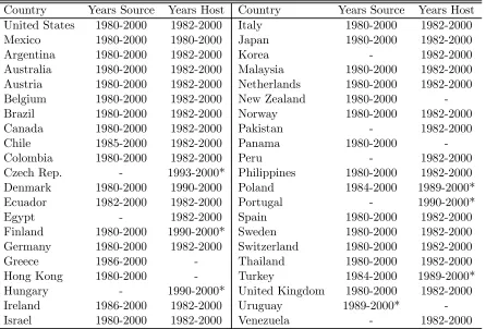
consists of countries other than the NAFTA countries that are hosts to U.S. FDI (see Table 3b

for a listing of countries and years included). We have chosen this control group largely because

it allows us to limit ourselves to just two data sources, the U.S. Bureau of Economic Analysis

(BEA) and the Mexican Statistical Institute (INEGI). The data section below will provide

more details on the data. The inclusion of other OECD countries would have required the use of

other data sources where comparability questions and thus mismeasurement loom large and may

(18)

by NAFTA. However, most U.S. outward FDI is in other highly-developed countries which are

quite dissimilar from Mexico and thus unlikely to contain many competing hosts. Secondly,

Bertrand et al. (2004) point out econometric problems in the use of the diﬀerence-in-diﬀerences

estimator. We discuss how we address these in the next section.

For other control variables to include in the empirical model, we appeal to the standard FDI

literature. We employ the most general speciﬁcation from Markusen and Maskus (2002) as our

base speciﬁcation. We also use similar speciﬁcations to those suggested in Blonigen et al., 2003,

Braconier et al., 2005, and Waldkirch, 2003.11

Thus, we augment the model by including the following controls:

F DI =f

⎛ ⎜ ⎜ ⎝

sumgdp,gdpdiﬀsq, d2skdgdpd, d2skdsumg, d1skdsumg,

invcosthost, topenhost, topensrc, distance

⎞ ⎟ ⎟

⎠ (12)

The ﬁrst term, sumgdp, is expected to be positive as larger combined market size will

encourage foreign production. The second term,gdpdiﬀsq, squared diﬀerences in GDP between

the host and the parent country of foreign investment, is expected to be negative as unequal-sized

countries should encourage exporting rather than setting up a plant in the foreign market.

The next three terms are more complicated interaction terms. The third term,d2skdgdpd,

interacts skill diﬀerences with GDP diﬀerences and a dummy equal to one if the skilled labor

abundant country is the parent country. Multinationals are discouraged if skill and GDP

dif-ferences are too large since the market of the small country is too small and the skilled labor

abundant parent country has a comparative advantage in (skill-intensive) headquarter services.

The other two terms are interactions of GDP sums and skill diﬀerences. The fourth term,

d2skdsumg, is again nonzero if the parent country is skilled-labor intensive. Skill diﬀerences

encourage vertical diﬀerentiation of the production process, but not horizontal multinationals,

since skill diﬀerences make skilled labor too expensive in that case. Therefore, its sign is

theoret-1 theoret-1_{For a detailed discussion of the knowledge-capital model and its empirical implementation, see Markusen’s}

(19)

ically ambiguous. The next term,d1skdsumg, is nonzero if the skilled labor abundant country

is the host country of investment. If this is the case, inward FDI is discouraged for all types of

multinationals since the skilled labor abundant country would be expected to be the parent, but

not the host country of investment. As a robustness check, we include simpler skill variables for

both source and host countries.

Four additional controls are included. First is a measure of the cost of investing in the host

country. It accounts for formal investment barriers as well as the overall economic climate that

aﬀects the decision where to invest. Higher investment costs deter FDI and hence a negative

sign is expected for this regressor. Parent country and host country (Mexican) trade costs are

measured by the ratio of exports plus imports to GDP, an often used measure for the trade

openness of a country. It is used over others because it is available for the entire sample period.

Since greater openness corresponds to lower trade costs, a positive sign is expected for parent

country, but a negative sign for host country trade costs.12 Finally, distance is measured as the

distance between country capitals. Its sign is theoretically ambiguous since it can proxy for both

trade and investment costs. It is included since it usually performs well in gravity-type models.

We should note that ascribing the eﬀects that weﬁnd solely to NAFTA is clearly problematic

as other events during the time period that we are looking at may aﬀect the pattern of FDI as

well and we have only limited ways to control for those. In addition to NAFTA, Mexico joined

the OECD in 1994, but more importantly, the 1994 peso crisis led to a steep real depreciation of

the peso, followed by a real appreciation in the years afterwards. We control for these eﬀects by

including Mexican GDP, which fell considerably in 1995. We could also include exchange rates

in order to account more directly for the monetary eﬀects of the crisis, but chose to follow real

trade theory and omit them.13

1 2

Endogeneity may be a concern with this openness measure. However, other measures such as an index from the Global Competitiveness Report are highly correlated with any measure of investment cost. In any case, omitting the openness variables does not change the qualitative results.

(20)

4 Econometric Considerations and Data

4.1 Econometric Considerations

The data are in panel form and preliminary tests indicated that both autocorrelation and

het-eroscedasticity were present. Therefore, we use a panel data model (Prais-Winsten regression)

with panel corrected standard errors. We report results from regressions where the

autocor-relation coeﬃcient is assumed to be diﬀerent for each observational unit (country pair). The

variance-covariance matrix is computed under the assumption that the disturbances are

het-eroscedastic and contemporaneously correlated across units, where each pair of cross-sectional

units has their own covariance. For each element in the covariance matrix, all available

obser-vations that are common to the two units contributing to the covariance are used to compute

it, given that the panel is unbalanced.14

We have an unbalanced panel because not all data are available for all years of the sample

period. We apply the following rules. Since we are primarily interested in the eﬀects of NAFTA,

we need suﬃcient data for both the pre- and the post-NAFTA time periods. We have at most

seven years of post-NAFTA data (1994-2000) and only use country-pair observations for which

we have at least seven years of pre-NAFTA information for all variables. In order to implement

the correction for autocorrelation, no gaps in the data are allowed. Hence, when there is a gap,

we limit ourselves to using post-gap information. In other words, if 1983 is available, 1984 is

missing, and 1985 onwards is available, the data for this country-pair starts in 1985. One of

the robustness checks uses a larger number of observations, although a minimum of ﬁve must

still be imposed in order to allow for the computation of the autocorrelation coeﬃcients for all

country pairs.

Bertrand et al. (2004) point out that ignoring serial correlation in diﬀerence-in-diﬀerences

1 4

(21)

estimation can lead to severely biased standard errors. While we account for the problem

by estimating a ﬁrst-order autocorrelation coeﬃcient, we also use one of the techniques they

suggest which works well for samples of more than 20 observational units (we have at least 70

country pairs). It requires estimating standard errors while allowing for an arbitrary covariance

structure between time periods, using a generalized White-like formula. This estimator of the

variance-covariance matrix is consistent as the number of country pairs tends to inﬁnity.

4.2 Data

Mexican FDI data come from the Mexican National Statistical Institute (INEGI). These are FDI

stocks in Mexico from 1980 on, published in U.S. dollars. In the empirical analysis, nominal

values are converted to real dollars using the U.S. producer price index for capital equipment.

The data distinguish ten source countries throughout the sample period. They account for about

90 percent of total FDI in Mexico. Since 1994, more source country and especially industry detail

is available, but since we need suﬃcient pre-1994 data, we cannot use the additional detail in

this study. No industry or additional source country detail is available retroactively for the time

before NAFTA.

For most of the 1980s, investmentﬂows exhibit large variation, for example around the time

of Mexico’s ﬁnancial crisis in the early 1980s, but do not increase much over time. They do

increase noticeably in the late 1980s and then a large and sustained increase occurs with the

inception of NAFTA. The ﬁrst substantial increase in FDI in the late 1980s and early 1990s

coincided with a major overhaul of Mexico’s investment laws in 1989. Many obstacles to foreign

investors, such as licensing requirements and restrictions pertaining to majority ownership, were

removed. This change reversed Mexico’s long-standing policy of reserving ownership in many

sectors to Mexican nationals or the Mexican state and encouraging foreign investment only in

(22)

and earlier than in many other countries in the region, substantial privatizations occurred. By

1994, the number of state-owned enterprises had decreased to only 80, down from 1155. However,

as Franko (1999: 158-61) points out, foreign investors participated in this sale only to a small

degree. FDI from privatization constituted only 7.9 percent of total FDI between 1990 and 1995.

Yet, during theﬁrst half of the 1990s, Mexico was the major recipient of FDI in Latin America.

Brazil subsequently surpassed Mexico in that role, mainly because Brazil’s major privatizations

occurred in the second half of the 1990s. Lately, greenﬁeld investment and acquisitions of local

ﬁrms have dominated in Mexico. In 1997, 62 percent of FDI consisted of international investors

acquiring local ﬁrms. According to CEPAL (1999), recent large acquisitions include several

banks, beverage and tobacco companies.

The United States has been the most important source country both before and after 1994.

Sizableﬂows have also originated in European Union countries and Japan. The share of North

American investment in Mexico has decreased since 1994, even though Canada’s share alone has

increased. The U.S. share has fallen from over 80 percent in the early 1980s to about 60 percent

since NAFTA took eﬀect. The vast majority of foreign investment originates in other developed

countries. The only sizable investment ﬂows from other countries are from South Korea and

India, the latter being largely a one-time large purchase of a Mexican steel company.

U.S. inward and outward FDI data come from the standard source used in most studies of

U.S. FDI, the Bureau of Economic Analysis (BEA). These data are described in detail elsewhere.

Figure 1 shows the evolution of FDI in Mexico and the United States since 1980.

Control variable data also come from standard sources. We use PPP-adjusted GDP data

from the Penn World Tables (6.1). Trade data come from the same source. For investment

costs, we use the comprehensive measure from Business Environment Risk Intelligence (BERI),

which is a composite measure of operations risk, political risk, and a remittance and repatriation

(23)

An important control variable in many studies is skill. The two most common sources of

skill data are the International Labor Organization (ILO) and the Barro/Lee data on schooling.

We use both in our analysis to ensure the robustness of our results. The ILO data measure the

number of workers in a particular occupation and characterize some as skilled, some as unskilled,

employing the skill deﬁnitions from Carr et al. (2001). A country’s skill level then is represented

by the share of skilled workers. Weﬁll in missing data using a linear trend between non-missing

years. For just a few countries, additional years areﬁlled in using the growth rate of the skilled

labor share between non-missing years. Alternatively, we use the Barro/Lee data on years of

schooling. These are available only in ﬁve-year intervals and we ﬁll in missing values using a

linear trend as well.15 Table 3a contains summary statistics; Table 1b lists the countries and

years, separately for host and source observations.

5 Results

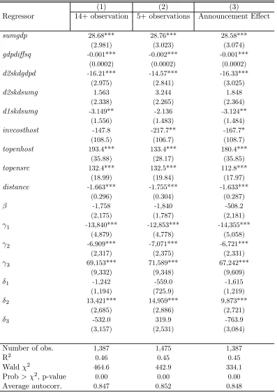
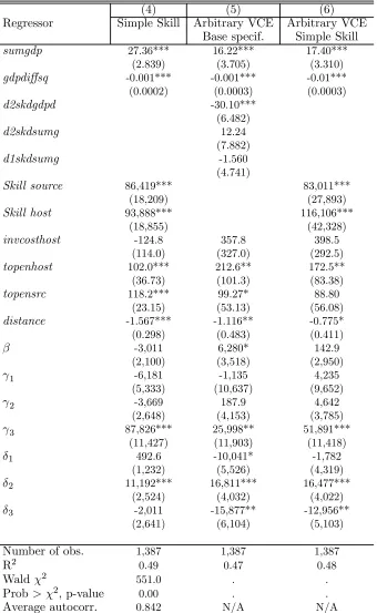
Tables 4-7 report the results. Tables 4a and 6a show the results from running a Prais-Winsten

regression as outlined above and Tables 4b and 6b contain robustness checks. Table 4 uses the

ILO skill data, while Table 6 uses the Barro/Lee skill data. Tables 5 and 7 present the simple

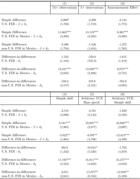
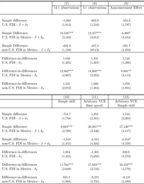
difference and the difference-in-differences estimation results, which are of central interest here.

The results reported in theﬁrst three rows of Tables 5 and 7 test Propositions 1-3. Speciﬁ

ca-tion (1) is our base speciﬁcation. The sample contains only source-host country pairs for which

we have at least 14 observations, i.e. suﬃcient pre- and post-NAFTA information. Speciﬁcation

(2) includes country pairs with fewer observations, which increases the sample size from 1,387

to 1,595 observations. However, many of the newly included country pairs still have twelve or

13 observations. Speciﬁcation (3) accounts for a possible announcement eﬀect by starting the

NAFTA regime dummy in 1992 rather than 1994.16

1 5_{Filling in missing values with repeated values from prior or future years does not change the results.}

(24)

Turning to Table 3, weﬁrst notice that there is only scant evidence of a FDI diversion eﬀect

from the U.S. since the eﬀect, while negative, is statistically signiﬁcant at only the ten percent

level in one speciﬁcation and then only when looking at the simple diﬀerence estimator (β+δ1).

It is not significant in any of the difference-in-differences results (δ1).17

This remains true for several robustness checks. Speciﬁcation (4) uses simple skill variables

instead of the complex interaction terms suggested by Markusen and Maskus (2002). We include

the share of skilled workers in the total workforce separately for host and source countries of

FDI. Speciﬁcations (5) and (6) use an alternative econometric technique, suggested by Bertrand

et al.’s (2004) concern about serial correlation in diﬀerence-in-diﬀerences estimations. While

the Prais-Winsten method corrects for serial correlation, Bertrand et al. (2004) show that

the correction may not be appropriate since it does not take into account second- or third-order

autocorrelation. Thus, we apply one of their suggested solutions, namely computing an arbitrary

variance-covariance matrix, to both our base speciﬁcation (1) and the speciﬁcation with simpler

skill terms. Results are shown in the bottom half of Table 5.

The diﬀerence-in-diﬀerences estimator for inward U.S. FDI is marginally negative in (5),

but not in any other speciﬁcation. When using the Barro/Lee skill data (Table 7), none of the

computed eﬀects on U.S. inward FDI are signiﬁcant. We thus conclude that there is at best

very weak evidence of a FDI diversion eﬀect from the U.S.

The next row of Tables 5 and 7 addresses FDI from the U.S. into Mexico. Here, there is a

statistically signiﬁcant and economically large positive eﬀect, suggesting that NAFTA has led

to an increase in FDI in Mexico from the U.S. Almost all coeﬃcients, whether simple diﬀerence

(β+δ2) or difference-in-differences (δ2), are significant at the one percent level, regardless of

speciﬁcation or skill data used. Thus, this is an extremely robust result. In order to get a sense

of the estimated economic eﬀect of NAFTA for U.S. investment in Mexico, we can calculate the

request.

1 7_{Calculating the economic e}_ﬀ_{ect from the point estimates reveals that, if signi}_ﬁ_{cant, NAFTA results in an}

(25)

predicted amount of FDI by theﬁnal year of the sample period with and without NAFTA. We

ﬁnd that this stock is about 24 percent higher than it would have been without NAFTA. We

stress again that this eﬀect includes events that we did not control for. Nonetheless, NAFTA

appears to have had an important eﬀect on U.S. FDI in Mexico.18

The ﬁnal row in Tables 5 and 7 shows the estimated NAFTA-eﬀect on FDI from

non-U.S. sources into Mexico. Here, the results are somewhat mixed. All twelve simple diﬀerence

estimates have a negative sign, four significantly so. Only two difference-in-differences estimates

are signiﬁcantly negative, the rest are not statistically signiﬁcant. We can conclude that we

cannot ﬁnd any evidence of an increase of non-U.S. FDI in Mexico due to NAFTA, although

there may have been a decrease. The reason appears to be that FDI from these sources was

much higher than implied by the usual determinants even before NAFTA was implemented, as

suggested by the uniformly large and signiﬁcantly positive coeﬃcient γ3, which indicates that

eﬀect.

The diﬀerential results with respect to U.S. and non-U.S. FDI into Mexico underscore the

importance of distinguishing between these two fundamentally diﬀerent sources of FDI. They

also conﬁrmﬁndings elsewhere using only Mexican data (Waldkirch, 2003, Cuevas et al., 2003).

The novel result here is that this is conﬁrmed when we add U.S. (inward and outward) data and

that there is little, if any, evidence of a FDI diversion eﬀect in the U.S.

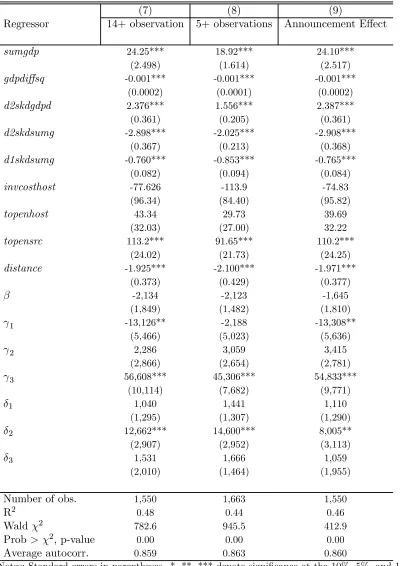
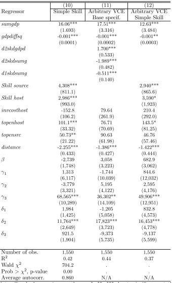
The determinants of FDI shown in the ﬁrst half of Tables 4a/4b and 6a/6b largely have

the expected signs and are statistically signiﬁcant, although the choice of skill data apparently

matters. As shown in other work, total market size has a large positive eﬀect on FDI, whereas

market size diﬀerences deter it. The signs on the skill variables are mostly consistent with

Markusen’s knowledge-capital model, although more so when using the ILO skill data.

Consis-1 8

(26)

tent with the predictions of that model, host country investment costs have a negative, source

country trade openness has a positive eﬀect, while the eﬀect of host country openness is more

ambiguous, though largely positive.

In summary, weﬁnd that NAFTA has aﬀected the location of North American FDI largely

by increasing U.S. FDI in Mexico. Other countries have been using Mexico as an export platform

well before NAFTA. There is hardly any evidence of FDI diversion from the U.S. The inclusion of

determinants of FDI that are well-established in the literature, a careful econometric speciﬁcation

that corrects for autocorrelation and heteroscedasticity, and the use of various measures of skill

endowments make us conﬁdent that our results provide a good assessment of the eﬀect of NAFTA

on the pattern of FDI in the United States and Mexico.

6 Conclusion and Directions for Future Work

This paper has investigated the eﬀect of the North American Free Trade Agreement on the

distribution of FDI in North America. We built a simple three-country model of location choice.

While the model is straightforward, it generates several interesting propositions. There is a

possibility that NAFTA results in FDI diversion from the United States. While FDI in Mexico

is likely to increase, the incentives forﬁrms from NAFTA partners versus non-partner countries

are aﬀected diﬀerently. This is due to the existence of the Maquiladora program before NAFTA,

but also to strict rules of origin and a possible commitment eﬀect that aﬀect partner countries

more than non-partner ones.

To our knowledge, this is the ﬁrst paper that combines both U.S. and Mexican FDI data to

test these hypotheses. Using a careful econometric analysis, we ﬁnd that U.S. FDI in Mexico

was positively aﬀected by NAFTA. At the same time, there is scant, if any, evidence of FDI

diversion from the U.S. Non-U.S. ﬁrms have been using Mexico as an export platform to the

(27)

of Mexico as a production location for these countries. If anything, FDI may have decreased.

These results are robust to the nature of the skill endowment data chosen, the consideration of

an “announcement” eﬀect as well as to the inclusion of country-pair observations with a shorter

time series. Moreover, we carefully take the serial correlation in the data into account and

employ speciﬁcations that avoid biasing our standard errors.

In future work, we will consider several extensions, both to the theory and the empirics.

The theory should incorporate plant-level scale economies through an integrated equilibrium

approach. In order to draw distinct conclusions, however, this will require numerical solutions.

We also envision a dynamic rather than a static game for economic integration, which will be

capable of including announcement and commitment eﬀects more formally.

On the empirical side, we note that even in its current form, our theoretical model also

provides a rich set of results regarding the eﬀect of NAFTA on trade within the region as well

as with other countries. These conclusions can be tested using available trade data. We are

(28)

References

[1] Bertrand, M., Duflo, E., Mullainathan, S., 2004. How Much Should we Trust Difference in Differences Estimates? Quarterly Journal of Economics 119(1), 249-75.

[2] Blonigen, B.A., Davies, R.B., Head, K., 2003. Estimating the Knowledge-Capital Model of the Multinational Enterprise: Comment. American Economic Review 93, 980-94.

[3] Blonigen, B.A., Davies, R.B., 2004. The Eﬀects of Bilateral Tax Treaties on U.S. FDI Activity. International Tax and Public Finance 11, 601-22.

[4] Braconier, H., Norbäck, P.-J., Urban, D., 2005. Multinational Enterprises and Wage Costs: Vertical FDI Revisited. Journal of International Economics 67, 446-70.

[5] Brainard, S.L., 1997. An Empirical Assessment of the Proximity-Concentration Trade-Oﬀ

between Multinational Sales and Trade. American Economic Review 87, 520-44.

[6] Carr, D.L., Markusen, J.R., Maskus, K.E., 2001. Estimating the Knowledge-Capital model of the Multinational Enterprise. American Economic Review 91, 693-708.

[7] CEPAL, 1999. Foreign Investment in Latin America and the Caribbean. 1998 Report. Santiago, Chile.

[8] Cuevas, A., Messmacher, M., Werner, A., 2005. Foreign Direct Investment in Mexico since the Approval of NAFTA. World Bank Economic Review 19, 473-88.

[9] Ekholm, K., Forslid, R., Markusen, J.R., 2007. Export-Platform Foreign Direct Investment. Journal of the European Economic Association 5, 776-95.

[10] Ethier, W.J., 1998. The New Regionalism. Economic Journal 108, 1149-1161.

[11] Feenstra, R.C., Hanson, G.H., 1997. Foreign Direct Investment and Relative Wages: Evi-dence from Mexico’s Maquiladoras. Journal of International Economics 42, 371-393.

[12] Fernandez-Arias, E. and Spiegel, M.M., 1998. North-South Customs Unions and Interna-tional Capital Mobility. Journal of InternaInterna-tional Economics 46, 229-251.

[13] Franko, P.M. 1999. The Puzzle of Latin American Economic Development. Rowman & Littleﬁeld, Lanham.

[14] Grossman, G.M., Helpman, E., Szeidl A., 2006. Optimal Integration Strategies for the Multinational Firm. Journal of International Economics 70, 216-38.

[15] Helpman, E., 1984. A Simple Theory of Trade with Multinational Corporations. Journal of Political Economy 92, 451-471.

[16] Markusen, J.R., 1984. Multinationals, Multi-Plant Economies, and the Gains from Trade. Journal of International Economics 16, 205-226.

[17] Markusen, J.R., 1997. Trade versus Investment Liberalization. NBER Working Paper Num-ber 6231.

(29)

[19] Markusen, J.R., Maskus, K.E., 2001. General-Equilibrium Approaches to the Multinational Firm: A Review of Theory and Evidence. NBER Working Paper Number 8334.

[20] Markusen, J.R., Maskus, K.E., 2002. Discriminating Among Alternative Theories of the Multinational Enterprise. Review of International Economics 10, 694-707.

[21] Motta, M., Norman, G., 1996. Does Economic Integration Cause Foreign Direct Investment? International Economic Review 37, 757-783.

[22] Waldkirch, A., 2003. The ‘New Regionalism’ and Foreign Direct Investment: The Case of Mexico. Journal of International Trade and Economic Development 12, 151-184.

[23] Waldkirch, A., 2006. The ‘New Regionalism’: Integration as a Commitment Device for Developing Countries. Journal of Economic Integration 21, 397-425.

(30)

(31)

[image:31.612.103.465.98.321.2]

Table 3a: Summary Statistics for Basic Speci

ﬁ

cation, Alternative Skill Measures

ILO skill measure Barro/Lee skill measure

Regressor Mean Median S.D. Mean Median S.D.

realfdi 12,542 2,088 26,918 11,110 1,682 25,163

sumgdp 6,404 6,743 2,361 6,546 6,795 2,357

gdpdiﬀsq 3.6E07 3.6E07 2.1E07 3.6E07 3.6E07 2.1E07

d2skdgdpd 213.6 0 517.6 11,251 0 17,132

d2skdsumg 355.4 81.49 533.3 13,607 0 19,668

d1skdsumg 314.6 0 523.1 16,523 1,959 20.670

invcosthost 39.99 31.67 13.84 39.37 31.67 13.45

topenhost 37.49 25.97 28.35 35.55 25.66 26.59

topensrc 43.80 29.55 36.39 43.27 31.76 34.64

distance 8,020 7,130 3,547 8,278 7,222 3,693

dNAFTA 0.45 0 0.50 0.46 0 0.50

dUShost 0.47 0 0.50 0.50 1 0.50

dMexhostUS 0.02 0 0.12 0.01 0 0.11

dMexhostnonUS 0.14 0 0.34 0.12 0 0.33

Table 3b: Countries and Years Included

Country Years Source Years Host Country Years Source Years Host

United States 1980-2000 1982-2000 Italy 1980-2000 1982-2000

Mexico 1980-2000 1980-2000 Japan 1980-2000 1982-2000

Argentina 1980-2000 1982-2000 Korea - 1982-2000

Australia 1980-2000 1982-2000 Malaysia 1980-2000 1982-2000

Austria 1980-2000 1982-2000 Netherlands 1980-2000 1982-2000

Belgium 1980-2000 1982-2000 New Zealand 1980-2000

-Brazil 1980-2000 1982-2000 Norway 1980-2000 1982-2000

Canada 1980-2000 1982-2000 Pakistan - 1982-2000

Chile 1985-2000 1982-2000 Panama 1980-2000

-Colombia 1980-2000 1982-2000 Peru - 1982-2000

Czech Rep. - 1993-2000* Philippines 1980-2000 1982-2000

Denmark 1980-2000 1990-2000 Poland 1984-2000 1989-2000*

Ecuador 1982-2000 1982-2000 Portugal - 1990-2000*

Egypt - 1982-2000 Spain 1980-2000 1982-2000

Finland 1980-2000 1990-2000* Sweden 1980-2000 1982-2000

Germany 1980-2000 1982-2000 Switzerland 1980-2000 1982-2000

Greece 1986-2000 - Thailand 1980-2000 1982-2000

Hong Kong 1980-2000 - Turkey 1984-2000 1989-2000*

Hungary - 1990-2000* United Kingdom 1980-2000 1982-2000

Ireland 1986-2000 1982-2000 Uruguay 1989-2000*

-Israel 1980-2000 1982-2000 Venezuela - 1982-2000

[image:31.612.106.552.391.693.2]

(32)

[image:32.612.106.503.98.659.2]

Table 4a: Prais-Winsten Regression Results: ILO Skill Data

(1) (2) (3)

Regressor 14+ observation 5+ observations Announcement Eﬀect

sumgdp 28.68*** 28.76*** 28.58***

(2.981) (3.023) (3.074)

gdpdiﬀsq -0.001*** -0.002*** -0.001***

(0.0002) (0.0002) (0.0002)

d2skdgdpd -16.21*** -14.57*** -16.33***

(2.975) (2.841) (3.025)

d2skdsumg 1.563 3.244 1.848

(2.338) (2.265) (2.364)

d1skdsumg -3.149** -2.136 -3.124**

(1.556) (1.483) (1.484)

invcosthost -147.8 -217.7** -167.7*

(108.5) (106.7) (108.7)

topenhost 193.4*** 133.4*** 180.4***

(35.88) (28.17) (35.85)

topensrc 132.4*** 132.5*** 112.8***

(18.99) (19.84) (17.97)

distance -1.663*** -1.755*** -1.633***

(0.296) (0.304) (0.287)

β -1,758 -1,840 -508.2

(2,175) (1,787) (2,181)

γ1 -13,840*** -12,853*** -14,355***

(4,879) (4,778) (5,058)

γ2 -6,909*** -7,071*** -6,721***

(2,317) (2,375) (2,331)

γ3 69,153*** 71,589*** 67,242***

(9,332) (9,348) (9,609)

δ1 -1,242 -559.0 -1,615

(1,194) (725.9) (1,219)

δ2 13,421*** 14,959*** 9,873***

(2,685) (2,886) (2,721)

δ3 -532.0 319.9 -763.9

(3,157) (2,531) (3,084)

Number of obs. 1,387 1,475 1,387

R2

0.46 0.45 0.45

Wald χ2

464.6 442.9 334.1

Prob> χ2

, p-value 0.00 0.00 0.00

Average autocorr. 0.847 0.852 0.848

Notes: Standard errors in parentheses. *, **, *** denote signiﬁcance at the 10%, 5%, and 1% level, respectively. All regressions include a constant and a time trend (not reported). Regressions correct for

(33)

[image:33.612.107.447.98.651.2]

Table 4b: Robustness Checks: ILO Skill Data

(4) (5) (6)

Regressor Simple Skill Arbitrary VCE Arbitrary VCE Base specif. Simple Skill

sumgdp 27.36*** 16.22*** 17.40***

(2.839) (3.705) (3.310)

gdpdiﬀsq -0.001*** -0.001*** -0.01***

(0.0002) (0.0003) (0.0003)

d2skdgdpd -30.10*** (6.482) d2skdsumg 12.24 (7.882) d1skdsumg -1.560 (4.741)

Skill source 86,419*** 83,011***

(18,209) (27,893)

Skill host 93,888*** 116,106***

(18,855) (42,328)

invcosthost -124.8 357.8 398.5

(114.0) (327.0) (292.5)

topenhost 102.0*** 212.6** 172.5**

(36.73) (101.3) (83.38)

topensrc 118.2*** 99.27* 88.80

(23.15) (53.13) (56.08)

distance -1.567*** -1.116** -0.775*

(0.298) (0.483) (0.411)

β -3,011 6,280* 142.9

(2,100) (3,518) (2,950)

γ1 -6,181 -1,135 4,235

(5,333) (10,637) (9,652)

γ2 -3,669 187.9 4,642

(2,648) (4,153) (3,785)

γ3 87,826*** 25,998** 51,891***

(11,427) (11,903) (11,418)

δ1 492.6 -10,041* -1,782

(1,232) (5,526) (4,319)

δ2 11,192*** 16,811*** 16,477***

(2,524) (4,032) (4,022)

δ3 -2,011 -15,877** -12,956**

(2,641) (6,104) (5,103)

Number of obs. 1,387 1,387 1,387

R2

0.49 0.47 0.48

Wald χ2

551.0 . .

Prob> χ2

, p-value 0.00 . .

Average autocorr. 0.842 N/A N/A

(34)

[image:34.612.104.568.96.691.2]

Table 5: The E

ﬀ

ect of NAFTA on North American FDI, ILO Skill Data

(1) (2) (3)

14+ observations 5+ observations Announcement Eﬀect

Simple diﬀerence -3,000* -2,399 -2,124

U.S. FDI -β+δ1 (1,780) (1,719) (1,773)

Simple Diﬀerence 11,663*** 13,119*** 9,365***

U.S. FDI in Mexico - β+δ2 (3,300) (3,382) (3,480)

Simple Diﬀerence -2,290 -1,520 -1,272

non-U.S. FDI in Mexico - β+δ3 (1,750) (1,616) (1,763)

Diﬀerence-in-diﬀerences -1,242 -559.0 -1,615

U.S. FDI -δ1 (1,194) (725.9) (1,219)

Diﬀerence-in-diﬀerences 13,421*** 14,959*** 9,873***

U.S. FDI in Mexico - δ2 (2,685) (2,886) (2,721)

Diﬀerence-in-diﬀerences -532.0 319.9 -763.9

non-U.S. FDI in Mexico - δ3 (3,157) (2,531) (3,084)

(4) (5) (6)

Simple skill Arbitrary VCE Arbitrary VCE Base specif. Simple skill

Simple diﬀerence -2,518 -3,761 -1,639

U.S. FDI -β+δ1 (2,090) (3,143) (2,528)

Simple diﬀerence 8,181*** 23,091*** 16,620***

Simple diﬀerence -5,022** -9,597** -12,813***

Diﬀerence-in-diﬀerences 492.6 -10,041* -1,782

U.S. FDI -δ1 (1,232) (5,526) (4,319)

U.S. FDI in Mexico - δ2 (2,524) (4,032) (4,022)

Diﬀerence-in-diﬀerences -2,011 -15,877** -12,956**

(35)

[image:35.612.106.506.98.664.2]

Table 6a: Prais-Winsten Regression Results: Barro/Lee Skill Data

(7) (8) (9)

Regressor 14+ observation 5+ observations Announcement Eﬀect

sumgdp 24.25*** 18.92*** 24.10***

(2.498) (1.614) (2.517)

gdpdiﬀsq -0.001*** -0.001*** -0.001***

(0.0002) (0.0001) (0.0002)

d2skdgdpd 2.376*** 1.556*** 2.387***

(0.361) (0.205) (0.361)

d2skdsumg -2.898*** -2.025*** -2.908***

(0.367) (0.213) (0.368)

d1skdsumg -0.760*** -0.853*** -0.765***

(0.082) (0.094) (0.084)

invcosthost -77.626 -113.9 -74.83

(96.34) (84.40) (95.82)

topenhost 43.34 29.73 39.69

(32.03) (27.00) 32.22

topensrc 113.2*** 91.65*** 110.2***

(24.02) (21.73) (24.25)

distance -1.925*** -2.100*** -1.971***

(0.373) (0.429) (0.377)

β -2,134 -2,123 -1,645

(1,849) (1,482) (1,810)

γ1 -13,126** -2,188 -13,308**

(5,466) (5,023) (5,636)

γ2 2,286 3,059 3,415

(2,866) (2,654) (2,781)

γ3 56,608*** 45,306*** 54,833***

(10,114) (7,682) (9,771)

δ1 1,040 1,441 1,110

(1,295) (1,307) (1,290)

δ2 12,662*** 14,600*** 8,005**

(2,907) (2,952) (3,113)

δ3 1,531 1,666 1,059

(2,010) (1,464) (1,955)

Number of obs. 1,550 1,663 1,550

R2

0.48 0.44 0.46

Wald χ2

782.6 945.5 412.9

Prob> χ2

, p-value 0.00 0.00 0.00

Average autocorr. 0.859 0.863 0.860

Notes: Standard errors in parentheses. *, **, *** denote signiﬁcance at the 10%, 5%, and 1% level, respectively. All regressions include a constant and a time trend (not reported). Regressions correct for

(36)

[image:36.612.107.447.97.657.2]

Table 6b: Robustness Checks: Barro/Lee Skill Data

(10) (11) (12)

Regressor Simple Skill Arbitrary VCE Arbitrary VCE Base specif. Simple Skill

sumgdp 16.06*** 17.51*** 12.63***

(1.693) (3.316) (3.484)

gdpdiﬀsq -0.001*** -0.001*** -0.001**

(0.0001) (0.0002) (0.0003)

d2skdgdpd 1.700*** (0.533) d2skdsumg -1.989*** (0.482) d1skdsumg -0.511*** (0.140)

Skill source 4,308*** 2,940***

(811.1) (865.6)

Skill host 2,986*** 3,590*

(993.0) (1,923)

invcosthost -152.8 79.64 210.4

(106.2) (261.9) (292.0)

topenhost 101.1*** 76.71 143.5*

(33.32) (70.69) (81.25)

topensrc 50.73** 90.63 46.76

(21.22) (61.98) (57.46)

distance -2.255*** -1.386*** -1.422***

(0.433) (0.427) (0.444)

β -2,739 3,058 682.9

(1,748) (3,223) (3,062)

γ1 1,313 -1,744 844.6

(6,117) (10,039) (12,032)

γ2 -3,779 5,195 2,595

(3,321) (4,122) (4,176)

γ3 68,565*** 36,302** 49,906***

(10,289) (14,109) (12,951)

δ1 1,984 -1,205 832.8

(1,425) (5,058) (4,573)

δ2 11,764*** 17,823*** 16,453***

(2,649) (3,723) (4,778)

δ3 921.5 -9,373 -9,137

(1,904) (5,735) (5,599)

Number of obs. 1,550 1,550 1,550

R2

0.42 0.44 0.37

Wald χ2

704.2 . .

Prob> χ2

, p-value 0.00 . .

Average autocorr. 0.860 N/A N/A

(37)

[image:37.612.103.568.97.690.2]

Table 7: The E

ﬀ

ect of NAFTA on North American FDI, Barro/Lee Skill Data

(7) (8) (9)

14+ observations 5+ observations Announcement Eﬀect

Simple diﬀerence -1,093 -682.9 -534.3

U.S. FDI -β+δ1 (1,813) (1,516) (1,797)

Simple Diﬀerence 10,528*** 12,477*** 6,360*

Simple Diﬀerence -602.3 -457.2 -585.7

non-U.S. FDI in Mexico - β+δ3 (1,129) (974.9) (1,253)

Diﬀerence-in-diﬀerences 1,040 1,441 1,110

U.S. FDI -δ1 (1,295) (1,307) (1,290)

Diﬀerence-in-diﬀerences 12,662*** 14,600*** 8,005**

U.S. FDI in Mexico - δ2 (2,907) (2,952) (3,113)

Diﬀerence-in-diﬀerences 1,531 1,666 1,059

(10) (11) (12)

Simple skill Arbitrary VCE Arbitrary VCE Base specif. Simple skill

Simple diﬀerence -754.7 1,853 1,516

U.S. FDI -β+δ1 (1,758) (2,561) (2,264)

Simple diﬀerence 9,024*** 20,881*** 17,136***

Simple diﬀerence -1,818 -6,315 -8,454*

Diﬀerence-in-diﬀerences 1,984 -1,205 832.8

U.S. FDI -δ1 (1,425) (5,058) (4,573)

U.S. FDI in Mexico - δ2 (2,649) (3,723) (4,778)

Diﬀerence-in-diﬀerences 921.5 -9,372 -9,137

(38)

[image:38.612.113.515.108.373.2]

Figure 1: FDI Stock in the United States and Mexico (billions of dollars)

0

50

0

10

00

15

0

US

0

50

10

0

15

0

Me

xi

co

1980 1985 1990 1995 2000 2005

Year

Mexico US

Source: For Mexico: INEGI; for the United States: Bureau of Economic Analysis