Threshold based Approach for Image Blind Deconvolution

Threshold based Approach for Image Blind

Deconvolution

Rachit Garg

Research Scholar Department of Computer Sc. National Institute of Technical Teachers Training & Research,

Chandigarh, India

Maitreyee Dutta,

Department of Computer Sc. National Institute of Technical Teachers Training & Research,

Chandigarh, India

Ramteke Mamta G

Research Scholar Department of Computer Sc. National Institute of Technical Teachers Training & Research,

Chandigarh, India

ABSTRACT

Having attractiveness in digital cameras, the digital image processing is getting more imperative nowadays. One of the most common problems facing with digital photography is noise and blurring that needs restoration. In this paper, we present a new method for image blind deconvolution [2]. The Proposed Method employs threshold based image restoration technique in blind image deconvolution. The goal of this work is to restore the image from a noisy and blurred image where the blurring function is not known. The blur process can be formulated as the image takes convolution operation with the Gaussian noise. One of the basic blind deconvolution method is an iterative blind deconvolution method. [5], [31]. Although Iterative Blind Deconvolution method can recover the image from blurred image, it is sensitive to initial estimation and computation time required is more. In order to decrease this computation time and better visual results than Iterative blind Deconvolution, we proposed a threshold based Blind image deconvolution algorithm.

General Terms

Blind Deconvolution, Non Blind Deconvolution, Peak Signal to Noise Ratio

Keywords

Non-Blind, Blind Deconvolution, PSF, PSNR, MSE, Computation Time, Threshold.

1.

INTRODUCTION

In any restoration there is a need of prior knowledge of degradation process also known as Point Spread Function, but in many situation PSF is unknown and image restoration involves estimation of PSF using some mathematical modeling, this approach is called as Blind Deconvolution. In this approach, both the degradation functions and true image are estimated from degraded image characteristics. The partial information about the imaging system may also be employed if available. Blind deconvolution is needed because in most of the practical cases, it is not possible to know the function that degrade the image. For example, in applications like astronomy and remote sensing, it is difficult to statistically model the original image or even know specific information about scenes never imaged before. In this paper we worked on Non-blind techniques [27], [28] and Iterative blind deconvolution method in order to compare the results of our proposed method.

2.

IMPLEMENTATION NON-BLIND

TECHNIQUE

2.1

Deconvolution by Weiner Filter (DWF)

Deconvolution with the use of Weiner Filter is the restoration approach of Non-blind category. The Wiener filter [1] purpose is to reduce the amount of noise present in a signal by comparison with an estimation of the desired noiseless signal. It is based on a statistical approach. Consider we need to design a wiener filter in a frequency domain as Restored image will be given as

(1)

Where is the received signal and is the restored image.

In order to simulate the image were convolved by Gaussian filter provided by MATLAB. The additive noise was simulated by using Gaussian Noise with variance 0.0002. The Wiener filtering is optimal in terms of the mean square error. In other words, the minimization of the overall MSE in the process of inverse filtering and smoothing of noise take place. The Wiener filtering is a linear estimation of the original image. The approach is based on a stochastic framework. Wiener filter in Fourier domain can be expressed as follows

(2)

Where, are power spectra of original

image and the additive noise respectively and is the blurring filter. The figure 1 shows the deconvolution results of Weiner filter.

(b)

(c)

(d)

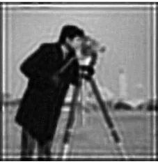
Fig 1: a) Original Image b) Blurred Image c) Blurred & Noisy Image d) Restored Image using Weiner Filter

Deconvolution

2.2

Deconvolution using Regularized Filter

(DRF)

Deconvolution by Regularized filtering [2] is another category of Non-Blind deconvolution technique. When constraints like smoothness are applied on the recovered image and limited information about the noise is known, then regularized deconvolution is used effectively. The degraded image is actually restored by constrained least square restoration by using a regularized filter. In regularized filtering less prior information is required to apply the restoration. Regularization can be a useful tool, when statistical data is unavailable. Moreover, this framework can be extended to adapt to edges of image, noise that is varying spatially and other challenges. The experiment for the same input image has been performed and the result of deconvolution is shown in figure 2.

Fig 2. Restored Image by Deconvolution by Regularized Filter

2.3

Deconvolution using Lucy Richardson

Algorithm (DLR)

The Richardson–Lucy algorithm, also known as Lucy– Richardson deconvolution, is an iterative procedure that restores the image that is blurred by known PSF. DLR [22] is a non-blind technique for restoration of image. It is used to restore a degraded image that has been blurred by a known PSF. The equation is given by

(3)

In the above equation di is the observed value at pixel position “ ”, is the PSF the fraction of light coming from true

location that is observed at position “i‟, is the latent image pixel value at location “ j‟. The main objective is to compute the most likely in the presence of observed and known PSF as follows:

(4)

(5)

The algorithm maximizes the likelihood which gives an image, by convolution with the PSF. It is an illustration of the blurred image, assuming Poisson noise information. This function works effectively when you know the PSF and also having partial knowledge about the additive noise in the image.

(6)

Where is the likelihood probability, the posteriori probability, and a prior model of the image. The experiment for the same input image has been performed and the result of deconvolution is shown in figure 3.

3.

IMPLEMENTATION BLIND

TECHNIQUE

3.1

Iterative Blind Deconvolution

Blind deconvolution is the approach of recovering an input blurry image when the blur kernel is unknown. Regular linear and non-linear deconvolution techniques utilize a known PSF.

In blind deconvolution, both the degradation function and the true image are estimated from the degraded image characteristics. Partial information about the imaging system may also be utilized if available. Like deconvlucy function, the deconvblind function also implements several adaptations to the original LR maximum likelihood algorithm that point complex image restoration jobs. Mathematically, we wish to decompose a blurred image y as

(7)

Where is a visually acceptable sharp image and is a non-negative blur kernel, whose support is small compared to the image size. This problem is rigorously ill-posed and there is an infinite set of pairs illustrating any observed . Recent algorithms have proposed to address the ill-posed problem of blind deconvolution by characterizing using natural image statistics [7], [8], [11], [12], [14].

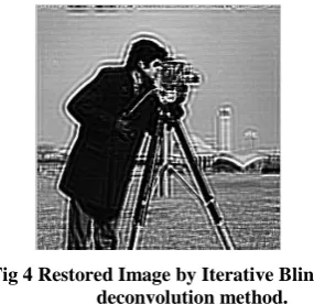
The simulated experiment for the input image has been performed and as a result of deconvolution is shown in figure 4.

Fig 4 Restored Image by Iterative Blind deconvolution method.

3.2

Deconvolution by Proposed

Methodology

One of the puzzling aspects of blind deconvolution is the failure of the MAP approach. Recent papers emphasized the usage of a sparse derivative prior to favors the sharp images. However, a direct application of this principle has not yielded the expected results and all algorithms required additional components, such as marginalization across all possible images [7],[11],[15] spatially-varying terms [8],[15] or solvers that vary their optimization energy over time [15]. We have analyzed the source of the MAP failure and during implementation of MAP, we come up with a novel approach of blind deconvolution for the restoration of Blurry and noisy image where the PSF is unknown.

The objective of proposed work is to restore the blurry and noisy image and compare the work with existing blind and non-blind algorithms. In our approach the blurred and noisy image is taken as input where the blurring parameters are unknown and it passes through the algorithm for the better results. Our approach is based on the threshold value taken into consideration. The image at various threshold values has

maximized and then replaced the value with values in blurred and noisy image. The replaced value has been calculated based on the threshold values. We compared our method with the Iterative Blind Deconvolution Techniques. Peak-Signal to Noise Ratio , Mean Square Error and Computation times has been taken as the parameters for the comparison and it was found that visual appearance of restored image from Our proposed method is found better and it takes less time in execution than Iterative blind deconvolution method. Figure 5 shows the result of restored image from proposed algorithm.

Fig 5Restored image with proposed algorithm

4.

RESULT AND ANALYSIS

Deconvolution by Various Blind and Non Blind have been performed and results has been shown in Fig 1,2,3,4,5 respectively. Computation Time has been measured for the considered categories of Blind and Non Blind Deconvolution Methods. It has been observed from our experiments that although the proposed method have PSNR value greater than

Proposed Algorithm

Step 1: Read input image X and convert into gray level matrix

Step 2: Find the maximum value of gray level.

Step 3: Estimate Initial threshold value.

Step 4: Initialize Y and K such that Y=max(X) and K=Y-threshold.

Step 5: for i = 1 to max_size

Compare pixel value with K

If pixel value less than K

Then new pixel value = pixel value

else new pixel value = Y

Step 6: Repeat the steps 1 to 5 until we converging to the desired output

proposed method is lesser than all the techniques. Table 2 shows the result of computation time for various techniques with respect to different size of the image and it was found that the proposed method has less computation time than other techniques as shown by fig 7 and visual appearance of restored image from deconvolution by proposed method is better than restored image from deconvolution by other considered techniques.

Table 1. Calculated parameters values for the various deconvolution techniques

DWF DRF DLR DIB Proposed

MSE 7411.60 4049.70 0.0081 0.0248 660.58

PSNR 9.47 12.0906 69.0978 64.2236 19.9656

Fig 6 PSNR Values

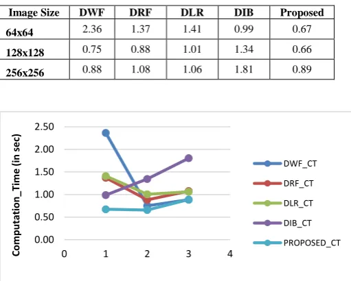
Table 2 Computation time for various methods of an image for different sizes

Image Size DWF DRF DLR DIB Proposed

64x64 2.36 1.37 1.41 0.99 0.67

128x128 0.75 0.88 1.01 1.34 0.66

256x256 0.88 1.08 1.06 1.81 0.89

Fig 7 Computation Time

5.

CONCLUSION

There is a rapid growth in true image restoration from blurred and noisy image. Digital Image Processing is widely used for this purpose. There are techniques available for the deconvolution of image which are categorized into two categories based on parameter Point Spread function PSF. One technique is the method of restoration of image with the knowledge of PSF which is known as Non-Blind and other is method of restoration of image without the knowledge of PSF which is known as Blind Deconvolution. This paper reports a threshold based novel approach for Blind Deconvolution.

Weiner Filter Deconvolution, regularized filter Deconvolution, Lucy Richardson method for deconvolution and Iterative Blind Deconvolution have been implemented as these are more commonly used methods for Digital Image Processing. These are analyzed against the parameters Execution Time, Peak Signal to Noise Ratio PSNR and ean Square Error MSE. Observations shows that computation time of our method is lesser than other considered methods. PSNR and MSE is better than DWF and DRF but it is not good as compared with DLR and DIB.

In future work PSNR for the DLR and DIB will be improved ad better results for visual appearance will also be achieved.

6.

REFERENCES

[1] B. Bocquet, R. Kit-Abdelmalek and Y. Leroy. 1993. Deconvolution and Weiner Filtering of Short range Radiometric Images. IEEE Electronics Letters, Vol. 29, Issue: 18, pp 1628-1629.

[2] Nicholas G. Paulter, Jr. 1994. A Casual Regularizing Deconvolution filter for optimal waveform Reconstruction. IEEE Transaction on Instrumentation and Measurement”, Vol. 43, Issue: 5, pp 740-747.

[3] Asoke K. Nandi, DetlefMampel and Burkhard Roscher. 1995 Comparative study of deconvolution algorithms with applications in non-destructive testing. IEEE Institute of Electrical Engineers, pp 1/1 - 1/6.

[4] Deepa Kundur and Dimitrios Hatzinakos. 1996. Blind Image Deconvolution. IEEE Signal Processing Magazine. Vol. 13, Issue: 3, pp 43-64.

[5] David S. C. Biggs and Mark Andrews.1997. Iterative blind Deconvolution of extended objects. IEEE International Conference on Image Processing, Vol. 2, pp 454-457.

[6] Dominikus Noll. 1997. Restoration of Degraded Images with Maximum Entropy. Journal of Global Optimization, Vol. 10, Issue: 1, pp 91-103.

[7] Yujiro Inouye and Takehito Sat. 1997. On-line Algorithms for Blind Deconvolution of Multichannel Linear Time-Invariant Systems. IEEE Signal Processing Workshop on Higher order Statistics, pp 204-208.

[8] Balvinder Singh and M. U. Siddiqi. 1997. MAP Estimation of Finite Gray-Scale Digital Images Corrupted by Supremum/Infimum Noise. IEEE Transaction on Image Processing, Vol. 6, No. 8 pp 1077-1088.

[9] Y. Yitzhaky and N. S. Kopeika.1998. Identification of Blur Parameters from Motion Blurred Images. ELSEVIER Journal of Graphical Models and Image, Vol. 59, Issue: 5, pp 310-320.

[10]H. Malcolm Hudson, Thomas C M Lee.1998. Maximum Likelihood restoration and choice of smoothing parameters in deconvolution of image data subject to Poisson noise. ELSEVIER Journal of Computational Statistics and data Analysis, Vol. 26 Issue: 4, pp 393-410.

[11]Deepa Kundur, Dimitrios Hatzinakos.1998. A Novel Blind Deconvolution Scheme for Image Restoration Using Recursive Filtering. IEEE Transaction on Signal Processing, Vol. 46, No. 2, pp 375-390.

0.00 20.00 40.00 60.00 80.00 PSNR PSNR_DWF PSNR_DRF PSNR_DLR PSNR_DIB PSNR_Proposed 0.00 0.50 1.00 1.50 2.00 2.50

0 1 2 3 4

C om put at ion_ Ti m e (i n se c)

IMAGE SIZE 1= 64x64, 2=128x128,3=256x256

DWF_CT

DRF_CT

DLR_CT

DIB_CT

[12]W. Miskin and D. J. C. MacKay.2000. Ensemble learning for blind image separation and Deconvolution. Springer Advances in Independent Component Analysis. pp 123-141.

[13]Boaz Cohen and lts'hak Dinstein. 2000. Motion Estimation in Noisy Ultrasound Images by Maximum Likelihood. 15th IEEE International Conference on Pattern recognition, Vol. 3 pp 182- 185.

[14]In Jae Myung. 2002. Tutorial on maximum likelihood estimation. Journal of Mathematical Psychology, Science Direct, Vol. 47 Issue: 1, pp 90-100.

[15]M. M. Bronstein, A. M. Bronstein, M. Zibulevsky, and Y. Y. Zeevi. 2005. Blind deconvolution of images using optimal sparse representations. IEEE Transactions on Image Processing , Vol. 14, Issue 6 pp 726–736.

[16]R. Fergus, B. Singh, A. Hertzmann, S.T. Roweis, and W.T. Freeman. 2006. removing camera shake from a single photograph. ACM Transaction on Graphics, Vol. 25, Issue: 3, pp 78-794.

[17]Anat Levin.2006. Blind motion deblurring using image statistics”, Conference on Advances in Neural Information Processing Systems (NIPS).

[18]Masayuki Tanaka, Kenichi Yoneji, and Masatoshi Okutomi.2007. Motion Blur Parameter Identification from a Linearly Blurred Image. IEEE International Conference on Consumer Electronics, pp 1-2.

[19]Leticia Vega-Alvarado, Izaskun Elezgaray, Agn Hémar, Michel Menard, Christophe Ranger Gabriel Corkidi. 2007. A comparison of image deconvolution algorithms applied to the detection of endocytic vesicles in fluorescence images of neural proteins. 29th _{IEEE Annual}

International Conference on Engineering in Medicine and Biology Society, pp 755-758.

[20]N. Joshi, R. Szeliski, and D. Kriegman. 2008. PSF Estimation using Sharp Edge Prediction. IEEE Conference on Computer Vision and Pattern Recognition, pp 1-8.

[21]Q. Shan, J. Jia, and A. Agarwala.2008. High-quality motion deblurring from a single image. ACM Transaction on Graphics, Vol. 27, Issue: 3, Article No. 73.

[22]Anat Levin, Yair Weiss, Fredo Durand, William T. Freeman.2009. Understanding and evaluating blind deconvolution algorithms. IEEE Conference on Computer Vision and Pattern Recognition, pp 1964- 1971.

[23]Li Dongxing, Han Jinhong and Xu Dong.2009. A Novel Restoration Algorithm of the Turbulence Degraded Images Based on Maximum Likelihood Estimation. 9th IEEE International Conference on Electronics Measurement and Instruments, pp 4-171 – 4-176.

[24]Feng DuanYanning Zhang.2009. The Estimation of Blur Based on Image Information. 5th IEEE International Conference on Image and Graphics, pp 109-112.

[25]Chao Wang, LiFeng Sun, Zhuo Yuan Chen, Shi Qiang Yang and Jian Wei Zhang. 2009. High quality non-blind

[26]Tal Kenig, ZviKam, and ArieFeuer.2010. Blind Image Deconvolution Using Machine Learning for Three-Dimensional Microscopy. IEEE Transaction on Pattern Analysis and Machine Intelligence, Vol. 32, Issue: 12, pp 2191-2204.

[27]Le Zou, Howard Zhou, Samuel Cheng and Chuan. 2010. Dual range deringing for non-blind image deconvolution. 17th IEEE International Conference on Image Processing, pp 1701-1704.

[28]Jong-Ho Lee and Yo-Sung Ho.2010. High-quality Non- Blind Image Deconvolution. 4th IEEE Pacific-Rim Symposium on Image and Video Technology, pp 282-287.

[29]Tingbo Hou, Sen Wang, Hong Qin , Rodney L. Miller. 2010. Image deconvolution using multigrid natural image prior and its applications. 17th IEEE International Conference on Image Processing, pp 3569-3572.

[30]Ms. S.Ramya, Ms. T.mercy Christial 2011. Restoration of blurred images using blind deconvolution algorithm. IEEE International Conference on Emerging trends in Electrical and Computer Technology ICETECT-2011, pp 496 -499.

[31]Lopamudra Kundu, Bhabatosh Chanda.2011. A Novel Iterative Blind Deconvolution using Morphology. 2nd IEEE International Conference on Emerging Applications of Information Technology, pp 181-184.

[32]Dilip Krishnan, Terence Tay and Rob Fergus.2011. Blind Deconvolution Using a Normalized Sparsity Measure. IEEE conference on Computer Vision and Pattern Recognition, pp 233-240.

[33]Sunghyun Cho, Jue Wang and Seungyong Lee.2011. Handling Outliers in Non-Blind Image Deconvolution. IEEE International Conference on Computer Vision, pp 495-502.

[34]Anat Levin, Yair Weiss, Fredo Durand, William T. Freeman. 2011. Efficient Marginal Likelihood Optimization in Blind Deconvolution. IEEE Conference on Computer Vision and Pattern Recognition, pp 2657-2664.

[35]Sudipto Dolui Oleg V. Michailovich 2011. Blind deconvolution of medical ultrasound images variable Splitting and proximal point methods.IEEE International Symposium on Biomedical Imaging from Nano to Macro, pp 1-5.

[36]Feng Xue and Thierry Blu.2012. Sure-based blind Gaussian deconvolution. IEEE Statistical Signal Processing Workshop (SSP), pp 452-455.

[37]Jiunn-Lin Wu, Chia-Feng Chang and Chun-Shih Chen.2012. An Improved Richardson-Lucy Algorithm for Single Image Deblurring Using Local Extrema Filtering. IEEE International Symposium on intelligent signal processing and communication system, pp 27-32.

[39]Wende Dong, Huajun Feng, Zhihai Xu, Qi Li.2013. Blind image deconvolution using the Fields of Experts prior. ELSEVIER Journal of Optics Communication Vol. 124, Issue: 18, pp 3601-3606.

[40] M. K. Khan, S. Morigi, L. Reichel and F. Sgallari. 2013. Iterative methods of Richardson-Lucy type for image deblurring. Journal of NUMERICAL MATHEMATICS: Theory, Methods and Applications, Vol. 6 pp 262-275.

[41]James Gregson Felix Heide Matthias Hulli Mushfiqur Rouf Wolfgang Heidrich. 2013. Stochastic Deconvolution. IEEE conference on computer Vision and Pattern Recognition, pp 1043-1050.

[42]Renaud Morin, Stephanie Bidonz, Adrian Basaraby, Denis Kouam.2013. Semi-blind deconvolution for resolution enhancement in ultrasound imaging. IEEE International Conference on Image Processing, pp 1413-1417.