Inferences for the Generalized Logistic Distribution Based on Record Statistics

http://dx.doi.org/10.4236/iim.2014.64018

Inferences for the Generalized Logistic

Distribution Based on Record Statistics

Rashad M. El-Sagheer

Mathematics Department, Faculty of Science, Al-Azhar University, Cairo, Egypt Email: [email protected], [email protected]

Received 28 April 2014; revised 27 May 2014; accepted 26 June 2014

Copyright © 2014 by author and Scientific Research Publishing Inc.

This work is licensed under the Creative Commons Attribution International License (CC BY).

http://creativecommons.org/licenses/by/4.0/

Abstract

Estimation for the parameters of the generalized logistic distribution (GLD) is obtained based on record statistics from a Bayesian and non-Bayesian approach. The Bayes estimators cannot be ob- tained in explicit forms. So the Markov chain Monte Carlo (MCMC) algorithms are used for compu- ting the Bayes estimates. Point estimation and confidence intervals based on maximum likelihood and the parametric bootstrap methods are proposed for estimating the unknown parameters. A numerical example has been analyzed for illustrative purposes. Comparisons are made between Bayesian and maximum likelihood estimators via Monte Carlo simulation.

Keywords

Generalized Logistic Distribution (GLD), Record Statistics, Parametric Bootstrap Methods, Bayes Estimation, Markov Chain Monte Carlo (MCMC), Gibbs and Metropolis Sampler

1. Introduction

Record values and the associated statistics are of interest and importance in many areas of real life applications involving data relating to meteorology, sport, economics, athletic events, oil, mining surveys and lifetesting. Many authors have studied records and associated statistics. Among them are Ahsanulla [1] [2], Resnick [3], Raqab and Ahsanulla [4], Nagaraja [5], Arnold et al. [6] [7], Raqab [8], Abd Ellah [9] [10], Sultan and Bala- krishnan [11], Preda and Panaitescu [12], Mahmoud et al. [13] and Sultan et al. [14].

Let X X1, 2,X3, a sequence of independent and identically distributed (iid) random variables with cumuli- tive distribution function F x

( )

and probability density function f x

( )

. Setting

(

1 2 3

)

min , , , , , 1

n n

Y = X X X  X n≥ we say that Xj is a lower record and denoted by XL j( ) if Yj <Yj−1, 1

The standard logistic distribution has important uses in describing growth and as a substitute for the normal distribution. It has also attracted interesting applications in the modeling of the dependence of chronic obstruct- tive respiratory disease prevalence on smoking and age, degrees of pneumoconiosis in coal miners, geological issues, hemolytic uremic syndrome data for children, physicochemical phenomenon, psychological issues, sur- vival time of diagnosed leukemia patients, and weight gain data. A generalized logistic distribution is proposed, based on the fact that the difference of two independent Gumbel distributed random variables has the standard logistic distribution. The generalized logistic distribution (GLD) has received additional attention in estimating its parameters for practical usage see for example Asgharzadeh [15]. The form of the probability density func- tion (pdf) and cumulative distribution function (cdf) of the two parameter generalized logistic distribution de- noted by GLD

(

λ θ,

)

are given, respectively, by

( )

(

(

)

)

( 1)

₍

₎

1 exp exp , , 0, 0,

f x =λθ + −θx − +λ −θx − ∞ < < ∞x λ> θ > ₍₁₎

( )

(

1 exp

(

)

)

, , 0, 0.

F x = + −θx −λ − ∞ < < ∞x λ> θ> ₍₂₎ Here λ and θ are the shape and scale parameters, respectively, the above GLD was originally proposed as a generalization of the logistic distribution by Johnson et al. [16]. For λ =1, the GLD becomes the standard lo- gistic and it is symmetric. The pdf in (1) has been obtained by compounding an extreme value distribution with a gamma distribution, different estimation procedures can be found in Chen and Balakrishnan [17].

The rest of the paper is organized as follows. In Section 2, we derive point estimation and the approximate confidence interval based on maximum likelihood estimation. The parametric bootstrap confidence intervals are discussed in Section 3. Section 4 describes Bayes estimates and construction of credible intervals using the MCMC algorithms. Section 5 contains the analysis of a numerical example to illustrate our proposed methods. A simula- tion studies are reported in order to give an assessment of the performance of the different estimation methods in Section 6. Finally we conclude with some comments in Section 7.

2. Maximum Likelihood Estimation

Suppose that x=xL_{( )}1,xL_{( )}2,,xL n_{( )} be the lower record values of size n from the generalized logistic distri-

bution GLD

(

λ θ,

)

. The likelihood function for observed record x _{was given by see Arnold} et al. [7]

(

)

( )

( )

( )

( ) ( )

( )

1 1 , , n L i L n i L i f x

x f x

F x

λ θ −

=

=

∏

 (3)

where f

( )

. and F

( )

. are given respectively, by (1) and (2), the likelihood function can be obtained by subs- tituting from (1) and (2) in (3) and written as

(

)

(

(

( )

)

)

( )

(

)

( )

(

)

1 exp

, 1 exp .

1 exp n L i n n L n i L i x x x x λ θ

λ θ λ θ θ

θ − = − = + − + −

∏

 ₍₄₎

The natural logarithm of the likelihood function (4) is given by

(

)

(

(

( )

)

)

( )

(

(

( )

)

)

1 1

, log log log 1 exp log 1 exp .

n n

L n L i L i

i i

L λ θ x n λ n θ λ θx θ x θx

= =

= + − + − −

∑

−

∑

+ − ₍₅₎

Differentiating (5) with respect to λ and θ and equating the results to zero, we obtain the likelihood equa- tions for the parameters λ and θ as

(

)

( )

(

)

(

)

,

log 1 exp L n 0,

L x _n

x λ θ θ λ λ ∂ = − + − =

∂ (6)

(

)

( )

(

( )

)

( )

(

)

(

)

( ) ( )

(

( )

)

( )

(

)

(

)

1 1 exp exp , 0.

1 exp 1 exp

n n

L n L n L i L i

L i

i i

L n L i

x x x x

L x _n

x

x x

λ θ θ

λ θ

θ θ _θ = = _θ

− −

∂

= + − + =

From (6), the maximum likelihood estimate (MLE) of λ say ˆλ, can be obtained as

( )

(

)

(

)

ˆ _.

log 1 exp _{L n}

n

x

λ

θ

=

+ − (8)

The MLE of the θ say ˆθ can be obtained by solving the non-linear likelihood equation

( )

( )

(

( )

)

( )

(

)

(

)

(

(

( )

)

)

( ) ( )

(

( )

)

( )

(

)

(

)

1 1 exp exp .

1 exp log 1 exp 1 exp

n n

L n L n L i L i

L i

i i

L n L n L i

nx x x x

n

f x

x x x

θ θ

θ

θ _{θ θ} = = _θ

− −

= + − +

+ − + −

∑

∑

+ − (9)

Therefore, ˆθ can be obtained as the solution of the non-linear equation in the form

( )

θ θ

Ψ = _{, (10)}

where

( )

( ) ( )

(

( )

)

( )

(

)

(

)

(

(

( )( )

)

)

(

(

( )

)

(

( )

)

)

1 1 1 exp exp

1 exp 1 exp log 1 exp

n n _{L i L i L n L n}

L i

i i

L i L n L n

x x nx x

n x

x x x

θ θ

θ

θ θ θ

−

= =

 _{− −} 

 

Ψ = _ − − _

+ − + − + −

 

 

∑

∑

(11)

Since ˆθ is a fixed point solution of non-linear Equation (9), therefore, it can be obtained by using a simple iterative scheme as follows

( )

θj θj+1,

Ψ = ₍₁₂₎

where θj is the thj iterate of ˆθ. The iteration procedure should be stopped when θˆj+1−θˆj is sufficiently

small. Once we obtain ˆθ from (9), and the MLE of λ say ˆλ becomes

( )

(

)

(

)

ˆ _.

ˆ log 1 exp _{L n}

n

x

λ

θ

=

+ − (13)

The asymptotic variance—covariance matrix of the maximum likelihood estimates for the two parameters λ and θ is the inverse of the Fisher information matrix after ignoring the expectation operators as following

( )

( )

( )

( )

(

)

(

)

(

)

(

)

( ) 1 2 2 2 2 2 2 , , ,

var cov ,

,

, ,

cov , var

L x L x

L x L x

λ θ

λ θ λ θ

λ λ θ _{λ λ θ}

λ θ λ θ

θ λ θ

θ λ θ

−  ∂ ∂  − −     ∂ ∂ ∂    _{ =}     _{∂ ∂}   − −   ∂ ∂ ∂        

   (14)

with

(

)

2 2 2 , ,

L λ θ x n

λ λ

∂

= −

∂ (15)

(

)

(

)

( )

(

( )

)

( )

(

)

(

)

2 2 _exp

, ,

, 1 exp

L n L n

L n

x x

L x L x

x θ

λ θ λ θ

λ θ θ λ _θ

−

∂ ∂

= =

∂ ∂ ∂ ∂ _{+ −} (16)

(

)

( )

(

)

(

( )

)

2 2 2 , , , ,

L n L i

L x _n

S x T x

λ θ

λ θ θ

θ θ

∂ ₋

= − −

∂ (17)

where ( )

(

)

( )

(

( )

)

( )

(

)

(

)

2 2 exp , , 1 exp

L n L n

L n L n x x S x x θ θ θ − =

( )

(

)

( )

(

( )

)

( )

(

)

(

)

2

2 1

exp

, .

1 exp

n

L i L i

L i i

L i

x x

T x

x

θ θ

θ

=

− =

+ −

∑

(19)

The asymptotic normality of the MLE can be used to compute the approximate confidence intervals for para- meters λ and θ. Therefore,

(

1−α

)

100% confidence intervals for parameters λ, and θ become, respec- tively, as

( )

( )

2 var and 2 var ,

Z_α Z_α

λ± λ θ± θ (20) where Zα2 is the percentile of the standard normal distribution with right-tail probability α 2.

3. Bootstrap Confidence Intervals

In this section, we propose to use confidence intervals based on the parametric bootstrap methods 1) percentile bootstrap method (Boot-p) based on the idea of Efron [18]; 2) bootstrap-t method (Boot-t) based on the idea of Hall [19]. The algorithms for estimating the confidence intervals using both methods are illustrated as follows.

3.1. Percentile Bootstrap Method

Algorithm 1

Step 1. From the original data x=xL_{( )}1,xL_{( )}2,,xL n_{( )} compute the ML estimates of the parameters λ

 and

θ by (13) and (9).

Step 2. Use λ and θ to generate a bootstrap sample x∗=x_L∗_{( )1},x_L∗_{( )2},,x∗_{L n( )}.

Step 3. As in Step 1, based on x∗ compute the bootstrap sample estimates of λ and θ, say λ∗ and θ∗. Step 4. Repeat Steps 2-3 N times representing N bootstrap MLE’s of λ and θ based on N different bootstrap samples.

Step 5. Arrange all λ∗′s and θ∗′s, in an ascending order to obtain the bootstrap sample

(

ϕ ϕ_l[ ]1, _l[ ]2,,ϕ_l[ ]N

)

, 1, 2

l= (where ϕ₁≡λ∗, ϕ₂ ≡θ∗).

Let G z

( )

=P

(

ϕ_l ≤z

)

be the cumulative distribution function of ϕl. Define

( )

1

lboot G z

ϕ ₌ −

for given z.

The approximate bootstrap 100 1

(

−α

)

% confidence interval of ϕl is given by

1 ,

2 2

lboot lboot

α α

ϕ ϕ

    − 

   

 _{   }

 . (21)

3.2. Bootstrap-t Method

Algorithm 2

Step 1. From the original data x=x_{L( )1},x_{L( )2},,x_{L n( )} compute the ML estimates of the parameters λ and

θ by Equations (13) and (9).

Step 2. Using λ and θ generate a bootstrap sample

{

xL_{( )}1,xL_{( )}2, ,xL n_{( )}

}

.

∗ ∗ ∗

 Based on these data, compute the bootstrap estimate of λ and θ, say λ∗ and θ∗ and following statistics

(

)

( )

(

( )

)

1 and 2

Var Var

n n

T T

λ λ θ θ

λ θ

∗ ∗

∗ ∗

∗ ∗

− −

= =

   

 

Step 4. For the T1 ∗

and T2 ∗

values obtained in Step 2, determine the upper and lower bounds of the

(

)

100 1−α % confidence interval of λ and θ as follows: let H x

( )

=P T

(

_i∗≤x

)

,i=1, 2 be the cumulative distribution function of T1

∗

and T2 ∗

. For a given x, define

( )

1 2

( )

1

( )

( )

1 2

( )

1

( )

- Var and - Var .

Boot t x n H x Boot t x n H x

λ _{= +}λ − λ − θ _{= +}θ − θ −

Here also, Var

( )

λ and Var

( )

θ can be computed as same as computing the Var

( )

λ∗ and Var

( )

θ∗ . The approximate 100 1

(

−α

)

% confidence interval of λ and θ are given by

- , - 1 and - , - 1 .

2 2 2 2

Boot t Boot t Boot t Boot t

α α α α

λ λ θ θ

    ₋      ₋           _{   }  _{   }         (22)

4. Bayes Estimation Using MCMC

In Bayesian approach, the performance depends on the prior information about the unknown parameters and the loss function. The prior information can be expressed by the experimenter, who has some beliefs about the un- known parameters and their statistical distributions. This section describes Bayesian MCMC methods that have been used to estimate the parameters of the generalized logistic distribution (GLD). The Bayesian approach is introduced and its computational implementation with MCMC algorithms is described. Gibbs sampling proce- dure [20] [21] and the Metropolis-Hastings (MH) algorithm [22] [23] are used to generate samples from the posterior density function and in turn compute the Bayes point estimates and also construct the corresponding credible intervals based on the generated posterior samples. By considering model (1), assume the following gamma prior densities for θ and λ as

(

)

( )

1

(

)

1

exp if 0

, ,

0 if 0 a

a

b

b

h θ a b a θ θ θ

θ

−



− > 

= Γ_

 _≤



(23)

and

(

)

( )

1

(

)

2

exp if 0

, .

0 if 0 c

c

d

d

h λ c d c λ λ λ

λ

−



− > 

= Γ_

 _≤



(24)

The joint prior density of λ and θ can be written as

(

)

(

) (

)

_{( ) ( )}

1 1

(

)

1 2

, , , exp .

a c

a c

b d

h h a b h c d b d

a c

λ θ ₌ θ λ ₌ θ λ− − ₋ θ₋ λ

Γ Γ (25)

Based on the likelihood function of the observed sample is same as (4) and the joint prior in (25), the joint posterior density of λ and θ given the data, denoted by h∗

(

λ θ, x

)

, can be written as

(

)

(

)

(

)

(

)

(

)

0 0

, ,

, ,

, , d d

x h

h x

x h

λ θ λ θ

λ θ

λ θ λ θ λ θ

∗ ∞ ∞ × = ×

∫ ∫



 (26)

therefore, the Bayes estimate of any function of λ and θ say g

(

λ θ,

)

, under squared error loss function is

(

)

(

)

(

)

(

)

(

)

(

)

(

)

0 0 ,

0 0

, , , d d

ˆ , , .

, , d d

x

g x h

g E g

x h

λ θ

λ θ λ θ λ θ λ θ

λ θ λ θ

λ θ λ θ λ θ

∞ ∞ ∞ ∞ × = _ _= ×

∫ ∫

∫ ∫



 (27)

4.1. MCMC Algorithm

The Markov chain Monte Carlo (MCMC) algorithm is used for computing the Bayes estimates of the parameters

λ and θ under the squared errors loss (SEL) function. We consider the Metropolis-Hastings algorithm, to generate samples from the conditional posterior distributions and then compute the Bayes estimates. The Me- tropolis-Hastings algorithm generate samples from an arbitrary proposal distribution (i.e. a Markov transition kernel). The expression for the joint posterior can be obtained up to proportionality by multiplying the likelihood with the joint prior and this can be written as

(

)

(

(

( )

)

)

( )

(

)

( )

(

)

1 1 1 exp

, exp log 1 exp ,

1 exp n

L i n c n a

L n i

L i

x

h d b x

x

θ

λ θ λ θ λ θ λ θ

θ ∗ + − + − = −   ∝ _− − − + − _

 

∏

_{+ −} (28)

from (28), the conditional posteriors distribution of parameter λ can be computed and written, by

( )

1

(

(

(

( )

)

)

)

1 exp log 1 exp .

n c

L n

h∗ λ θ ∝λ + − _−λ d+ + −θx _

  (29)

Therefore, the conditional posteriors distribution of parameter λ, is gamma with parameters

(

n+c

)

and

( )

(

)

(

)

(

d+log 1 exp+ −θx_{L n}

)

and, therefore, samples of λ can be easily generated using any gamma generat- ing routine.

The conditional posteriors distribution of parameter θ can be written as

( )

1

(

(

( )

)

)

( )

(

(

( )

)

)

2

1 1

exp log 1 exp log 1 exp .

n n

n a

L n L i L i

i i

h∗ θ λ θ + − bθ λ θx θ x θx

= =

 

∝ _− − + − − − + − _



∑

∑

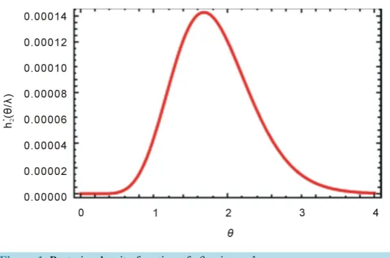
 (30)

The conditional posteriors distribution of parameter θ Equation (30) cannot be reduced analytically to well known distributions and therefore it is not possible to sample directly by standard methods, but the plot of it (see

Figure 1) show that it is similar to normal distribution. So to generate random numbers from this distribution, we use the Metropolis-Hastings method with normal proposal distribution. The choice of the hyper parameters

, ,

a b c and d which make (30) close to the proposal distribution and obviously more convergence of the MCMC iteration. We propose the following MCMC algorithm to draw samples from the posterior density func- tions; and in turn compute the Bayes estimates and also, construct the corresponding credible intervals.

Algorithm 3

Step 1. θ₀ =θ, M =nburn.

Step 2. Generate λ1 from gamma distribution h1

( )

λ θ . ∗

Step 3. Generate θ1 from h2

( )

θ λ ∗

using (MH) algorithm in [22] [23].

Step 4. Compute λ( )t and θ( )t . Step 5. Repeat Steps 2-4 N times.

Step 6. Obtain the Bayes estimates of λ and θ with respect to the SEL function as

( )

1 1 , N i i M E x N M λ λ = + = −

∑



_{( )}

1 1 . N i i M E x N M θ θ = + = −

∑



Step 7. To compute the credible intervals of λ and θ, λ1,,λN order and θ1,,θN as λ( )1 <<λ( )N

and θ_{( )1} <<θ_{( )N} . Then the 100 1

(

−α

)

% symmetric credible intervals of λ and θ become

( )2

(

( )1 2

)

( )2

(

( )1 2

)

, and , .

Nα N α Nα N α

λ λ ₋ θ θ ₋

   

   

    (31)

5. Numerical Computations

Figure 1. Posterior density function of θ given λ.

tively, λ =3 and β =2, as follows: 1.0509, 0.0780, −0.1271, −0.1892, −0.6437, −1.0886, −1.1212. Based on these lower upper record values, we compute the approximate MLEs, Bootstrap (Boot-p, Boot-t) and Bayes es- timates of λ and θ using MCMC algorithm, we assume that informative priors a=2.1,b=1.5,c=3.2 and

1.55

[image:7.595.173.458.81.269.2]

d= on both λ and θ. The density function of h₂∗

( )

θ λ given in (30) is plotted Figure 1. It can be approximated by normal distribution function as mentioned in Subsection 4.1. Also the 95%, approximate maximum likelihood estimation (AMLE) confidence intervals, Bootstrap confidence intervals and approximate credible intervals based on the MCMC samples are computed. The results are given in Table 1. Figure 2 and

Figure 3 plot the MCMC output of λ and θ, using 10 000 MCMC samples (dashed line represent means and red lines represent lower and upper bounds of 95% probability intervals). The plot of histogram of λ and θ generated by MCMC method are given in Figure 4 and Figure 5. This was done with 1000 bootstrap sample and 10,000 MCMC sample and discard the first 1000 values as “burn-in”.

6. Simulation Study and Comparisons

In this section, we conduct some numerical computations to compare the performances of the different estima- tors proposed in the previous sections. Monte Carlo simulations were performed utilizing 1000 lower record samples from a two-parameter generalized logistic distribution (GLD) for each simulation. The mean square er- ror (MSE) is used to compare the estimators. The samples were generated by using

(

λ θ,

) (

= 2,1.2

)

,

(

3.22,1.5

)

, with different sample of sizes

( )

n . For computing Bayes estimators, we used the non-informative gamma priors for both the parameters, that is, when the hyper parameters are 0. We call it prior 0:

0

a= = = =b c d . Note that as the hyper parameters go to 0, the prior density becomes inversely proportional to its argument and also becomes improper. This density is commonly used as an improper prior for parameters in the range of 0 to infinity, and this prior is not specifically related to the gamma density. For computing Bayes estimators, other than prior 0, we also used informative prior, including prior 1, a=1, b=2, c=2 and

1

d= , also we used the squared error loss (SEL) function to compute the Bayes estimates. We also computed the Bayes estimates and 95% credible intervals based on 10,000 MCMC samples and discard the first 1000 val- ues as “burn-in”. We report the average Bayes estimates, mean squared errors (MSEs) and coverage percentages. For comparison purposes, we also computed the MLEs and the 95% confidence intervals based on the observed Fisher information matrix. Finally, we used the same 1000 replicates to compute different estimates Tables 2-5

report the results based on MLEs and the Bayes estimators (using MCMC algorithm) on both λ and θ.

7. Conclusions

Figure 2. Trace plot MCMC output of λ.

Figure 3. Trace plot MCMC output of θ.

[image:9.595.95.537.409.700.2]

Figure 5. Histogram of θ generated by MCMC method.

Table 1. Results obtained by MLE, Bootstrap and MCMC method of λ and θ.

Method Parameter Point Interval Length

MLEs λ 3.0047 [−0.2232,6.2325] 6.4557

θ 1.9865 [0.1956,3.7774] 3.5817

Boot-p λ 2.9316 [1.6633,3.9486] 2.2852

θ 2.0012 [1.1767,2.9481] 1.7714

Boot-t λ 3.1591 [3.0250,4.8306] 1.8057

θ 2.1924 [1.1922,3.4791] 2.2869

MCMC λ 2.8700 [1.2621,5.2139] 3.9519

θ 1.8946 [0.9046,3.2826] 2.3779

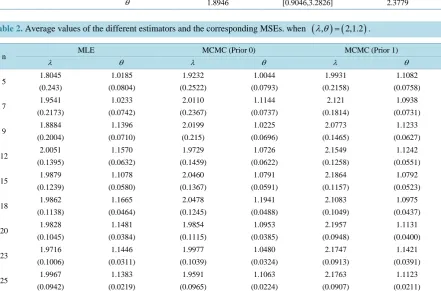
Table 2. Average values of the different estimators and the corresponding MSEs. when

(

λ θ,

) (

= 2,1.2

)

.

n MLE MCMC (Prior 0) MCMC (Prior 1)

λ θ λ θ λ θ

5 1.8045 1.0185 1.9232 1.0044 1.9931 1.1082

(0.243) (0.0804) (0.2522) (0.0793) (0.2158) (0.0758)

7 1.9541 1.0233 2.0110 1.1144 2.121 1.0938

(0.2173) (0.0742) (0.2367) (0.0737) (0.1814) (0.0731)

9 1.8884 1.1396 2.0199 1.0225 2.0773 1.1233

(0.2004) (0.0710) (0.215) (0.0696) (0.1465) (0.0627)

12 2.0051 1.1570 1.9729 1.0726 2.1549 1.1242

(0.1395) (0.0632) (0.1459) (0.0622) (0.1258) (0.0551)

15 1.9879 1.1078 2.0460 1.0791 2.1864 1.0792

(0.1239) (0.0580) (0.1367) (0.0591) (0.1157) (0.0523)

18 1.9862 1.1665 2.0478 1.1941 2.1083 1.0975

(0.1138) (0.0464) (0.1245) (0.0488) (0.1049) (0.0437)

20 1.9828 1.1481 1.9854 1.0953 2.1957 1.1131

(0.1045) (0.0384) (0.1115) (0.0385) (0.0948) (0.0400)

23 1.9716 1.1446 1.9977 1.0480 2.1747 1.1421

(0.1006) (0.0311) (0.1039) (0.0324) (0.0913) (0.0391)

25 1.9967 1.1383 1.9591 1.1063 2.1763 1.1123

(0.0942) (0.0219) (0.0965) (0.0224) (0.0907) (0.0211)

[image:10.595.94.537.112.386.2]

Table 3. The average confidence lengths relative estimate of parameters and the corresponding coverage percentages when

(

λ θ,

) (

= 2,1.2

)

.

n MLE MCMC (Prior 0) MCMC (Prior 1)

λ θ λ θ λ θ

5 4.8702 2.4925 3.9902 2.8843 3.895 1.8332

(0.945) (0.932) (0.947) (0.939) (0.941) (0.944)

7 4.7022 2.3674 3.9165 2.7655 3.8132 1.6703

(0.951) (0.945) (0.949) (0.952) (0.957) (0.961)

9 4.6367 2.3167 3.8037 2.6514 3.7922 1.6412

(0.948) (0.961) (0.950) (0.947) (0.962) (0.955)

12 4.5491 2.2694 3.6974 2.5728 3.6816 1.6245

(0.952) (0.945) (0.935) (0.947) (0.951) (0.948)

15 4.4749 2.2076 3.6741 2.4502 3.6548 1.5628

(0.946) (0.935) (0.947) (0.954) (0.948) (0.943)

18 4.3877 2.1902 3.5398 2.3935 3.5167 1.5056

(0.955) (0.932) (0.940) (0.941) (0.934) (0.945)

20 4.2899 2.1206 3.3972 2.3739 3.4720 1.4860

(0.957) (0.960) (0.952) (0.963) (0.949) (0.951)

23 4.1493 2.0834 3.3104 2.2731 3.4250 1.3359

(0.947) (0.950) (0.939) (0.961) (0.956) (0.942)

25 3.9063 1.9875 3.1455 2.1301 3.1112 1.2858

(0.944) (0.953) (0.955) (0.950) (0.961) (0.949)

Note: The first figure represents the average confidence lengths, with the corresponding coverage percentages reported below it in parentheses.

Table 4. Average values of the different estimators and the corresponding MSEs when

(

λ θ,

) (

= 3.22,1.5

)

.

n MLE MCMC (Prior 0) MCMC (Prior 1)

λ θ λ θ λ θ

5 3.2188 1.536 3.2428 1.5141 3.1885 1.6195

(0.3966) (0.1007) (0.4165) (0.1042) (0.3878) (0.0951)

7 3.3344 1.4766 3.1343 1.4757 3.2048 1.4382

(0.3356) (0.0945) (0.3522) (0.0946) (0.2991) (0.0915)

9 3.1654 1.4312 3.1273 1.4812 3.1491 1.5037

(0.2832) (0.0876) (0.2914) (0.0879) (0.2507) (0.0765)

12 3.0307 1.4325 3.2107 1.4301 3.2125 1.4789

(0.2599) (0.0778) (0.2509) (0.0781) (0.2184) (0.0723)

15 3.3056 1.4989 3.2191 1.4418 3.2116 1.4698

(0.1910) (0.0615) (0.1962) (0.0629) (0.1693) (0.0588)

18 3.2708 1.5056 3.2027 1.4691 3.1473 1.4733

(0.1734) (0.0574) (0.1885) (0.0583) (0.1233) (0.0462)

20 3.2311 1.5006 3.1915 1.4984 3.2360 1.4139

(0.1161) (0.0463) (0.1351) (0.0495) (0.0952) (0.0341)

23 3.1083 1.5203 3.2963 1.5485 3.2186 1.5506

(0.0848) (0.0182) (0.0946) (0.0177) (0.0508) (0.0101)

25 3.2571 1.5921 3.2216 1.574 3.2757 1.4958

(0.0713) (0.0097) (0.0721) (0.0098) (0.0363) (0.0074)

[image:10.595.97.538.422.703.2]

[image:11.595.97.538.114.374.2]

Table 5. The average confidence lengths relative estimate of parameters and the corresponding coverage percentages when

(

λ θ,

) (

= 3.22,1.5

)

.

n MLE MCMC (Prior 0) MCMC (Prior 1)

λ θ λ θ λ θ

5 5.1771 3.5337 5.1266 3.3999 4.6647 2.5659

(0.954) (0.943) (0.948) (0.936) (0.951) (0.947)

7 5.1173 3.4583 5.0925 3.3214 4.6213 2.3181

(0.952) (0.938) (0.940) (0.936) (0.951) (0.939)

9 5.0559 3.3879 5.0618 3.2440 4.4488 2.2556

(0.955) (0.948) (0.939) (0.961) (0.947) (0.954)

12 5.0164 3.3633 5.0247 3.2027 4.3837 2.1898

(0.946) (0.951) (0.947) (0.953) (0.938) (0.949)

15 4.9628 3.2716 4.9799 3.1927 4.2322 2.1307

(0.952) (0.956) (0.948) (0.933) (0.949) (0.950)

18 4.7335 3.1509 4.7563 3.1384 4.1996 2.0984

(0.954) (0.947) (0.955) (0.951) (0.944) (0.946)

20 4.4643 3.1286 4.4889 3.1281 4.0891 1.9796

(0.962) (0.952) (0.959) (0.961) (0.953) (0.942)

23 4.2226 3.0712 4.2475 3.0835 4.0354 1.7458

(0.961) (0.948) (0.949) (0.945) (0.952) (0.956)

25 4.1321 3.0216 4.1350 3.0291 3.9818 1.5514

(0.958) (0.946) (0.945) (0.960) (0.957) (0.951)

Note: The first figure represents the average confidence lengths, with the corresponding coverage percentages reported below it in parentheses.

[27] presented Bayesian estimation for the generalized Logistic distribution Type-II censored accelerated life testing. In this paper Bayesian estimation for the parameters of the generalized logistic distribution (GLD) are computed based on the lower record values using MCMC method. We assume the gamma priors on the un- known parameters and provide the Bayes estimators under the assumptions of squared error loss functions (SEL). The Metropolis-Hastings (MH) algorithm from the MCMC method is used for computing Bayes estimates. It has been noticed that,

1) From the results obtained in Tables 2-5, it can be seen that the performance of the Bayes estimators with respect to the non-informative prior (prior 0) is quite close to that of the MLEs, as expected. Thus, if we have no prior information on the unknown parameters, then it is always better to use the MLEs rather than the Bayes es- timators, because the Bayes estimators are computationally more expensive.

2)Tables 2-5report the results based on non-informative prior (prior 0) and informative prior, (prior 1) also in these case the results based on using MH algorithm are quite similar in nature when comparing the Bayes es- timators based on informative prior clearly shows that the Bayes estimators based on prior 1 perform better than the MLEs, in terms of MSEs.

3) From Tables 2-5, it is clear that the Bayes estimators based on informative prior perform much better than noninformative prior and the MLEs in terms of MSEs.

Acknowledgements

The author would like to express their thanks to the editor, assistant editor and referees for their useful com- ments and suggestions on the original version of this manuscript.

References

[1] Ahsanullah, M. (1993) On the Record Values from Univariate Distributions. National Institute of Standards and Tech- nology Journal of Research, Special Publications, 12, 1-6.

[2] Ahsanullah, M. (1995) Introduction to Record Statistics. NOVA Science Publishers Inc., Huntington.

http://dx.doi.org/10.1007/978-0-387-75953-1

[4] Raqab, M.Z. and Ahsanulla, M. (2001) Estimation of the Location and Scale Parameters of the Generalized Exponen- tial Distribution Based on Order Statistics. Journal of Statistical Computation and Simulation, 69, 109-124.

http://dx.doi.org/10.1080/00949650108812085

[5] Nagaraja, H.N. (1988) Record Values and Related Statistics—A Review. Journal of Communication in Statistics The- ory and Methods, 17, 2223-2238. http://dx.doi.org/10.1080/03610928808829743

[6] Arnold, B.C. (1983) Pareto Distributions. In: Statistical Distributions in Scientific Work, International Co-Operative Publishing House, Burtonsville.

[7] Arnold, B.C., Balakrishnan, N. and Nagaraja,H.N.(1998) Records. Wiley, New York. http://dx.doi.org/10.1002/9781118150412

[8] Raqab, M.Z. (2002) Inferences for Generalized Exponential Distribution Based on Record Statistics. Journal of Statis- tical Planning and Inference, 52, 339-350. http://dx.doi.org/10.1016/S0378-3758(01)00246-4

[9] Abd Ellah, A.H. (2011) Bayesian One Sample Prediction Bounds for the Lomax Distribution. Indian Journal of Pure and Applied Mathematics, 42, 335-356.

[10] Abd Ellah, A.H.(2006) Comparison of Estimates Using Record Statstics from Lomax Model: Bayesian and Non Baye- sian Approaches. Journal of Statistical Research and Training Center, 3, 139-158.

[11] Sultan, K.S. and Balakrishnan, N. (1999) Higher Order Moments of Record Values from Rayleigh and Weibull Distri- butions and Edge worth Approximate Inference. Journal of Applied Statistical Sciences, 9, 193-209.

[12] Preda, V. and Panaitescu, E. (2010) Estimations and Predictions Using Record Statistics from the Modified Weibull Model. WSEAS Traning of Mathematics, 9, 427-437.

[13] Mahmoud, M.A.W., Soliman, A.A., Abd Ellah, A.H. andEL-Sagheer, R.M. (2013) Markov Chain Monte Carlo to Study the Estimation of the Coefficient of Variation. International Journal of Computer Applications, 77, 31-37. [14] Sultan, K.S., AL-Dayian, G.R. and Mohammad, H.H. (2008) Estimation and Prediction from Gamma Distribution

Based on Record Values. Computational Statistics & Data Analysis, 52, 1430-1440. http://dx.doi.org/10.1016/j.csda.2007.04.002

[15] Asgharzadeh, A. (2006) Point and Interval Estimation for a Generalized Logistic Distribution Under Progressive Type II Censoring. Communications in Statistics-Theory and Methods, 35, 1685-1702.

http://dx.doi.org/10.1080/03610920600683713

[16] Johnson, N.L., Kotz, S. and Balakrishnan, N. (1995) Continuous Univariate Distributions. 2nd Edition, Wiley and Sons, New York.

[17] Chen, G. and Balakrishnan, N. (1995) The Infeasibility of Probability Weighted Moments Estimation of Some Genera- lized Distributions. In: Balakrishnan, N., Ed., Recent Advances in Life-Testing and Reliability, CRC Press, Boca Raton. [18] Efron, B. (1982) The Bootstrap and Other Resampling Plans. In: CBMS-NSF Regional Conference Series in Applied

Mathematics, SIAM, Philadelphia.

[19] Hall, P. (1988) Theoretical Comparison of Bootstrap Confidence Intervals. Annals of Statistics, 16, 927-953. http://dx.doi.org/10.1214/aos/1176350933

[20] Geman, S. and Geman, D. (1984) Stochastic Relaxation, Gibbs Distributions and the Bayesian Restoration of Images.

IEEE Transactions on Pattern Analysis and Machine Intelligence, 12, 609-628. http://dx.doi.org/10.1109/34.56204 [21] Smith, A. and Roberrs, G. (1993) Bayesian Computation Via the Gibbs Sampler and Related Markov Chain Monte

Carlo Methods. Journal of the Royal Statistical Society, 55, 3-23.

[22] Metropolis, N., Rosenbluth, A.W., Rosenbluth, M.N., Teller, A.H. and Teller, E. (1953) Equations of State Calcula- tions by Fast Computing Machine. Journal Chemical Physics, 21, 1087-1091. http://dx.doi.org/10.1063/1.1699114 [23] Hastings, W.K. (1970) Monte Carlo Sampling Methods Using Markov Chains and Their Applications. Biometrika, 57,

97-101. http://dx.doi.org/10.1093/biomet/57.1.97

[24] Rezaei, S., Tahmasbi, R. and Mahmoodi,M. (2010) Estimation of P[Y<X] for Generalized Pareto Distribution. Jour- nal of Statistical Planning and Inference, 140, 480-494. http://dx.doi.org/10.1016/j.jspi.2009.07.024

[25] Upadhyaya, S.K. and Gupta, A. (2010) A Bayes Analysis of Modified Weibull Distribution Via Markov Chain Monte Carlo Simulation. Journal of Statistical Computation and Simulation, 80, 241-254.

http://dx.doi.org/10.1080/00949650802600730

[26] Amin, A. (2012) Bayesian and Non-Bayesian Estimation from Type I Generalized Logistic Distribution Based on Lower Record Values. Journal of Applied Sciences Research, 8, 118-226.

currently publishing more than 200 open access, online, peer-reviewed journals covering a wide range of academic disciplines. SCIRP serves the worldwide academic communities and contributes to the progress and application of science with its publication.

Other selected journals from SCIRP are listed as below. Submit your manuscript to us via either