JPEG Image Compression using DCT and DHT and Comparison of Both Techniques based on Mean Square Error and Peak Signal to Noise Ratio

(1)

JPEG Image Compression using DCT and DHT and

Comparison of Both Techniques based on Mean Square

Error and Peak Signal to Noise Ratio

Dhananjay Patel

Assistant Professor, Don Bosco Institute of

Technology, Mumbai

Alina Menoth Jose

B.E. Student Don Bosco Institute Of

Technology,Mumbai

Steape Stany Monis

Technology,Mumbai

Nigel Mascarenhas

Technology,Mumbai

ABSTRACT

DCT based JPEG compression is a widely used standard for lossy image compression. DCT concentrates energy into lower order coefficients. It removes redundancy between neighbouring pixels which leads to uncorrelated transform coefficients which can be encoded independently. There is high computational complexity in DCT. DHT is a real valued transform whose forward and inverse transforms are same except for a an inclusion of a scale factor in the inverse transform. DHT reduces the computational complexity of JPEG compared to DCT. DHT doesn’t require a dequantizer at the decoder, since a new quantization technique known as energy quantization is used. It speeds up the encoding procedure, reduces hardware as well as makes the implementation simpler. The quality of the reconstructed image is very good which is verified using MATLAB i.e. the PSNR is improved and the MSE is reduced.

Keywords

Discrete Cosine Transform (DCT), Discrete Hartley Transform (DHT), Joint Photographic Experts Group (JPEG), Quantization, Encoding, Peak Signal to Noise Ratio(PSNR), Mean Square Error(MSE)

1. INTRODUCTION

Image compression is useful both for transmission and storage of information [3]. Image contains a high degree of redundancy which makes it possible for compression of an image. They are as follows: (1) redundancy due to correlation between neighbouring pixels, (2) redundancy due to properties of HVS (human visual system). Image compression system consists of transformer, quantizer and encoder. The transformer transforms the raw image data from one domain to another domain. The quantizer standardizes these transformed coefficients [2]. The encoder provides a code word to each symbol of fixed length or variable length. DHT follows the same approach of the JPEG compression and reconstruction but employs a different transform. We have compared the performance of both DCT and DHT based JPEG compression through MATLAB. The comparison has been made in terms of Peak Signal to Noise Ratio (PSNR) and MSE of the compressed and reconstructed image.

2. TECHNIQUES OF IMAGE

COMPRESSION

2.1 JPEG Compression Using DCT

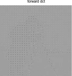
The image is first partitioned into different blocks. Discrete Cosine Transform (DCT) is applied to each of the blocks to convert from spatial domain to frequency domain. [1] The transform coefficients using the DHT of a block of pixels x(m, n) may be obtained as

N j y N i x y x p j C i C N j i D N x N y 2 ) 1 2 ( cos 2 ) 1 2 ( cos ) , ( ) ( ) ( 2 1 ) , ( 1 0 1 0     



   

Where p(x,y) is the x,yth _{element of the image represented by} the matrix p. N is the size of the matrix on which the DCT is applied.

Hence small set of coefficients are obtained. The DCT coefficients are quantized using a quantization matrix provided by JPEG standard. The JPEG quantizer consists of 64 uniform quantizers.

The i’th quantizer is calculated as

Yi=Round (Xi/Qi)

where Qi is the i’th quantization step size, Xi is the input and Yi is the quantized version of Xi. After quantization the quantized coefficients are arranged in a zigzag order that is arranged in lowest to highest spatial frequency. Then a lossless coding technique that is, Run-length coding is applied to further compress the data. The decoding is just the inverse of encoding process. [1]

2.2 JPEG Compression Using DHT

The forward and inverse transforms are same in DHT along with an inclusion of a scale factor in its inverse transform. Besides, the DHT can compute both convolution and the DFT efficiently. The memory requirement to compute both the forward and inverse DHT is about half as those of the DCT [10]. The transform coefficients using the DHT of a block of pixels x(m, n) may be obtained as



               _      _         _      _   1 0 1 0 ln 2 sin ln 2 cos ) , ( ) , ( N n M

m M N

(2)

Volume 81 – No 15, November 2013` Where k=0,1,....M-1 and l=0,1,...N-1, x(m,n) represents the

block of pixels on which theDHT is calculated . The Inverse Discrete Hartley Transform may be obtained as





 

 

 

 

   



 _

   

 _

     



 _

   

 _



 1

0 1

0

ln 2

sin ln 2 cos ) , ( ) / 1 ( ) , (

N n

M

m M N

km N

M km n

m x MN l k X

Where k=0,1,....M-1 and l=0,1,...N-1.[7]

DHT coefficients do not follow zigzag scanning; they follow a special scanning . So the designing of the Quantization matrix is quite difficult in DHT. To eliminate these difficulties, energy quantization is used.

3. ENERGY QUANTIZATION

A signal is a function of amplitude versus time. On squaring the signal amplitudes gives rise to the energy contribution. The energy of the transformed coefficients of the image block can be obtained by adding all the signals

If the energy of the transformed coefficient is less than the threshold value then make it zero, otherwise keep the coefficient as it is. The threshold value is decided according to the user requirement, i.e. how much energy of the image user wants to save. For higher compression and low quality, maximum amount of the energy has to be discarded [8]. First the normalized energy of the transformed coefficients is calculated using





 







1

0 1

0

2 )

,

(

)

/

1 (

M

m N

n

m

x

MN

En

where M and N are the width and length of the sample block and x(m,n) is the transformed samples. Then energy of the transformed coefficient wrt. threshold value is considered. The DHT coefficient can be saved as it is, but the transformed coefficients have been normalized to decrease the amplitudes. At the decoder the compressed data is dequantized and passed through the IDHT operation to reconstruct the image[8].

Figure 01: Block diagram of a JPEG Encoder

[image:2.595.370.488.414.564.2]

Table 1: Scanning order of DHT coefficient

4. EXPERIMENTAL RESULTS

The Peak Signal to Noise Ratio (PSNR) is calculated using

)

/

(

log

20

10

Max

MSE

PSNR



Where, Max =255,







 





M

y N

x

y

x

I

y

x

I

MN

MSE

1

2

1

)

,

(

'

)

,

(

1

Where I(x,y) and I’(x,y) are the original and compressed pixel values respectively, and (M×N) is the image size[8].

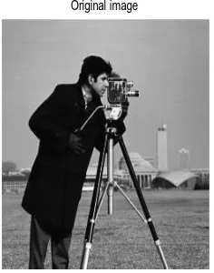
[image:2.595.52.312.499.620.2]

The DCT and DHT programs are implemented using Matlab. The performance of DCT and DHT on lossy JPEG compression is compared. The PSNR and MSE values are calculated for different images as shown below.

Figure 02: Original image Original image

1 2 4 6 8 10 12 14

3 16 17 19 21 23 25 27

5 18 29 30 32 34 36 38

7 20 31 40 41 43 45 47

9 22 33 42 49 50 52 54

11 24 35 44 51 56 57 59

13 26 37 46 53 58 61 62

15 28 39 48 55 60 63 64

8*8 block sourc e image

Forwar

d DCT Quantiz_er Entrop_y

encod er

Compress ed image data

Quantizatio n table

(3)

Figure 03: Compressed image using DCT

Figure 04: Reconstructed image using DCT

[image:3.595.99.236.78.224.2]

Figure 05: Compressed image using DHT

[image:3.595.330.530.307.488.2]

Figure 06: Reconstructed image using DHT

Figure 07: Comparison of MSE of Compressed Image w.r,t DCT and DHT (for cameraman.jpg)

Figure 08: Comparison of MSE of Reconstructed Image with DCT and DHT (for cameraman.jpg)

forward dct

RECONSTRUCTED IMG

Forward DHT

0 50 100 150 200 250 300

0 0.5 1 1.5 2 2.5 3 3.5

4x 10 5

pixel intensity

M

S

E

MSE COMPARISON OF COMPRESSED IMAGE

mse of encoded dct mse of encoded dht

0 50 100 150 200 250 300

0.7 0.8 0.9 1 1.1 1.2 1.3x 10

6

pixel intensity

M

S

E

MSE COMPARISON OF RECONSTRUCTED IMAGE

mse of decoded dct mse of decoded dht

(4)

[image:4.595.62.300.83.257.2]

Volume 81 – No 15, November 2013`

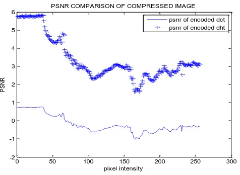
[image:4.595.320.550.85.259.2]

Figure 09: Comparison of PSNR of Compressed Image with DCT and DHT (for cameraman.jpg)

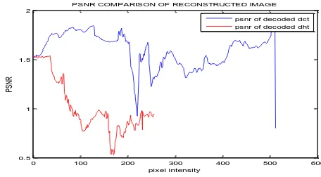
Figure 10: Comparison of PSNR of Reconstructed Image with DCT and DHT (for cameraman.jpg)

Figure 11: Comparison of MSE of Compressed Image with DCT and DHT (for lena.jpg)

Figure 12: Comparison of MSE of Reconstructed Image with DCT and DHT (for lena.jpg)

Figure 13: Comparison of PSNR of Compessed Image with DCT and DHT (for lena.jpg)

Figure 14: Comparison of PSNR of Reconstructed Image with DCT and DHT (for lena.jpg)

0 50 100 150 200 250 300

-2 -1 0 1 2 3 4 5 6

pixel intensity

P

S

N

R

PSNR COMPARISON OF COMPRESSED IMAGE psnr of encoded dct psnr of encoded dht

0 50 100 150 200 250 300

-1 -0.5 0 0.5 1 1.5 2

pixel intensity

P

S

N

R

PSNR COMPARISON OF RECONSTRUCTED IMAGE

psnr of decoded dct psnr of decoded dht

0 50 100 150 200 250 300

0 0.5 1 1.5 2 2.5

3x 10

5

pixel intensity

M

S

E

MSE COMPARISON OF COMPRESSED IMAGE

mse of encoded dct mse of encoded dht

0 50 100 150 200 250 300

7.5 8 8.5 9 9.5 10 10.5 11 11.5x 10

5

pixel intensity

M

S

E

0 50 100 150 200 250 300

0 1 2 3 4 5 6

pixel intensity

P

S

N

R

PSNR COMPARISON OF COMPRESSED IMAGE

psnr of encoded dct psnr of encoded dht

0 50 100 150 200 250 300

0 0.2 0.4 0.6 0.8 1 1.2 1.4 1.6

pixel intensity

P

S

N

R

[image:4.595.320.538.518.705.2]

(5)

[image:5.595.57.286.66.232.2]

Figure 15: Comparison of MSE of Compressed Image with DCT and DHT (for usair.jpg)

[image:5.595.326.554.68.194.2]

Figure 16: Comparison of MSE of Reconstructed Image with DCT and DHT (for usair.jpg)

Figure 17: Comparison of PSNR of Compressed Image with DCT and DHT (for usair.jpg)

Figure 18: Comparison of PSNR of Reconstructed Image with DCT and DHT (for usair.jpg)

5. CONCLUSION

In this paper, compression of image is carried out using DCT and DHT. Using MATLAB, the PSNR and MSE of compressed and reconstructed image is found out. While comparing the results on compressed and reconstructed images using DCT and DHT, it can be found that the PSNR is improved using the DHT technique and the mean square error is reduced using DHT technique. Also, the concept of energy quantization used in DHT technique is explained which comes into picture in the DHT scanning.

6. REFERENCES

[1] Gopal Lakhani, Optical Huffman coding of DCT Blocks IEEE transactions on circuits and systems for video technology, VOL.14,NO.4,April 2004.

[2] En-hui Yang,Fellow, IEEE and Longji Wang, Joint Optimization Of Run-Length Coding, Huffman Coding, and Quantization Table with Complete Baseline JPEG Decoder Compatibility, IEEE transactions on image processing, VOL. 18,NO.1,JANUARY 2009.

[3] Gopal Lakhani,Modified JPEG Huffman Coding IEEE transactions on Image Processing, VOL.12, NO.2, February 2003.

[4] D.Malarvizhi, Dr.K.Kuppusamy, A New Entrophy Encoding Algorithm For Image Compression Using DCT, International Journal of Engineering Trends and Technology- Volume3Issue3- 2012.

[5] Maneesha Gupta, Dr.Amit Kumar Garg ,Analysis Of Image Compression Algorithm Using DCT, International Journal of Engineering Research and Applications (IJERA), Vol. 2, Issue 1, Jan-Feb 2012,pp.515-521. [6] H. S. Hou, "The fast Hartley Transform algorithm", IEEE

Trans. on Computer, vol. 36, no. 2, pp. 147-156, Feb. 1987.

[7] Sorensen ,Jones, Burrus, Heideman, ”Computing the discrete Hartley transform”,Acoustics,Speech and Signal Processing,IEEE transactions,Vol.33.

[8] Sharma,Agarwal,Pati,Mohapatr,a2-D Separablediscrete Hartley transform architecture for efficient FPGA resource,Iinternational Coference on Computer And Communication Technology,2010

[9] Sai Lakshmi Kumari N, U.Pradeep Kumar, K.V.Ramana Rao, Implementation of 2D Hartley transform using Distributed Arithmetic, International Journal of Innovative Technology and Exploring Engineering (IJITEE), Volume-1, Issue-5, October 2012.

0 100 200 300 400 500 600

0.2 0.4 0.6 0.8 1 1.2 1.4 1.6 1.8

2x 10

5

pixel intensity

M

S

E

MSE COMPARISON OF COMPRESSED IMAGE mse of encoded dct mse of encoded dht

0 100 200 300 400 500 600

7 7.5 8 8.5 9 9.5 10 10.5x 10

5

pixel intensity

M

S

E

0 100 200 300 400 500 600

1.5 2 2.5 3 3.5 4 4.5 5 5.5 6

pixel intensity

P

S

N

R

PSNR COMPARISON OF COMPRESSED IMAGE

psnr of encoded dct psnr of encoded dht

0 100 200 300 400 500 600

0.5 1 1.5 2

pixel intensity

PS

NR

[image:5.595.64.277.285.470.2]