Human Capital Formation and Patterns of Growth with Multiple Equilibria

Munich Personal RePEc Archive

Human Capital Formation and Patterns

of Growth with Multiple Equilibria

Mino, Kazuo

Institute of Economic Research, Kyoto University

2003

Human Capital Formation and Patterns of Growth with

Multiple Equilibria

Kazuo Mino2

July 2003

1_{An earlier version of this paper was presented at the Taipei International Conference on Economic}

Growth held at Academia Sinica in December, 1999. I wish to thank the participants of the conference, especially, Danyang Xie, the discussant of the paper, for their valuable comments and advices. I also thank the anonymous referees whose comments are very helpful in preparing the …nal version of the paper. All remaining errors are, of course, mine. Financial support from Nihon Keizai Kenkyu Shorei Zaidan is gratefully acknowledged.

Abstract

1

Introduction

This paper examines a model of endogenous growth with multiple equilibria. Our main concern is to demonstrate that growth models with multiple converging paths may present a useful analytical framework to consider various growth patterns among the countries that have similar economic environments. Of course, it is not novel to use growth models with multiple equilibria for describing diverse growth patterns. The presence of low-growth trap generated by multiplicity of long-run equilibria has been a popular idea in development economics. In particular, the argument about ’history versus expectations’ emphasized by Krugman (1991) and Matsuyama (1991) has been discussed extensively. A common feature in this class of studies is that indeterminacy holds under the assumption of strong degree of increasing returns.1 _{However, the recent empirical investigations suggest that the degree}

of increasing returns may not be so large as many theoretical studies have assumed. This implies that the exposition of non-convergence of per-capita income and diverse patterns of growth based on indeterminacy of equilibrium would be empirically dubious.

In this paper we demonstrate that the presence of increasing returns is not necessary for generating indeterminacy of equilibrium. By using one of the prototype models of endogenous growth, we show that multiple equilibria and complex patterns of transitional dynamics can emerge even under social constant returns. The main purpose of examining such a model is to emphasize that we do not need extreme assumptions to show diverse growth performances among the countries with similar technologies and preferences. If we make a small modi…cation of the base model in which equilibrium should be unique, the model will display various patterns of growth dynamics.

More speci…cally, we analyze a generalized version of the two-sector endogenous growth models à la Lucas (1988). We show that if the utility function of the representative family is not additively separable between consumption and leisure and if there are sector-speci…c externalities, then the Lucas model may produce indeterminacy of equilibrium even if tech-nologies of the …nal good and the new human capital production sectors satisfy social constant returns. In order to clarify the analysis, we impose speci…c conditions on the parameter val-ues involved in the model. This enables us to examine global dynamic behavior of the model.

We demonstrate that in this speci…c case the balanced growth equilibrium may be locally indeterminate. Additionally, the model may involve dual balanced-growth equilibria. If the economy involves dual long-run equilibria, the balanced-growth equilibrium with a higher growth rate is locally determinate, while the other with a lower growth rate may be locally indeterminate. In this case, the global dynamics of the model economy is rather complex: un-der the same initial condition, the identical economies will follow completely di¤erent growth processes depending on expectations of the economic agents.

In the existing literature, Benhabib and Perli (1994) and Xie (1994) explore indetermi-nacy in the Lucas model. Xie (1994) presents a detailed analysis of transitional dynamics in the presence of indeterminacy by setting speci…c conditions on parameter values of the model. Since he treats a model without labor-leisure choice, indeterminacy needs strong in-creasing returns. Benhabib and Perli (1994) consider endogenous labor supply and show that indeterminacy can be established with relatively small degree of increasing returns. They use an additively separable utility function, so that indeterminacy stems from speci…c production structure assumed in their model. In contrast to these contributions, this paper emphasizes the role of preference structure in generating indeterminacy.

It is to be noted that Benhabib, Meng and Nishimura (1999) and Mino (1999b) also examine indeterminacy in the two-sector endogenous growth models with social constant returns. A key assumption in their models is that both …nal good and new human capital producing sectors use human as well as physical capital. In this setting, they show that local indeterminacy holds, if the …nal good sector is more human capital intensive than the new human capital producing sector from the private perspective but it is more physical capital intensive from the social perspective.2 Since the Lucas model used in this paper assumes that the education sector employs human capital alone, there is no factor intensity reversal between the social and the private technologies (the …nal good sector always uses a more physical capital intensive technology than the education sector). Therefore, the cause of indeterminacy with social constant returns in this paper mainly comes from the preference structure rather than from the production technology emphasized by Benhabib, Meng and

2_{Since they assume that there is no labor-leisure choice, the balanced-growth equilibrium is uniquely}

Nishimura (1999) and Mino (1999b).3

The rest of the paper is organized as follows. Section 2 sets up the model. Section 3 derives the dynamical system and examines local dynamics. Based on the simpli…ed model, Section 4 characterizes global dynamics and presents some economic implications of our main results. In Section 5 points out the limitation of our analysis and the issues to be explored for strengthen the empirical plausibility of our claims.

2

The Model

2.1 Production

Consider a competitive economy with two production sectors. The …rst sector produces a …nal good that can be used either for consumption or for investment on physical capital. The production technology is given by

Y1 =K H₁1K1"H11; ; 1 >0; + 1+"+ 1= 1; (1)

where Y1 denotes the …nal good, K is stock of physical capital and H1 is human capital

devoted to the …nal good production. K" _{and H} 1

1 represent sector-speci…c externalities

associated with physical and human capital employed in this sector.4 The key assumption in (1) is that the production technology is socially constant returns to scale. The second sector is an education sector that produces new human capital. Following the Lucas-Uzawa setting, we assume that new human capital production needs human capital alone and its technology is speci…ed as

Y2 = H12H22; ; 2; 2>0; 2+ 2= 1: (2)

Here, Y2 is newly produced human capital, H2 is the stock of human capital used in the

education sector, and H 2

2 stands for sector speci…c externalities. Again, the production

technology of new human capital exhibits social constant returns.

3_{Pelloni and Waldmann (2000) emphasize the role of non-separable utility function for generating}

indeter-minacy in one-sector endogenous growth model based on Romer (1986). In a one-sector economy endogenous growth can be sustained in the presence of large degree of increasing returns, so that not only non-separability of utility function but also increasing returns are crucial for showing indeterminacy in Pelloni and Waldmann (2000).

The …rms in each sector maximize their pro…ts under given external e¤ects. Thus the value of marginal product of each private capital equals to its nominal rent:

R=p1 K 1H11K1"H11; (3)

W =p_{1 1}K H 1 1

1 K1"H11 =p2 2H22 1H22; (4)

whereR; W; p1 andp2 respectively denote the nominal rent on physical capital, the nominal

rent on human capital, the price of …nal good and the price of new human capital. Note that since the private technologies exhibit decreasing returns, the …rms may earn positive pro…ts. We assume that entire stocks of physical and human capital are owned by the households so that the pro…ts are distributed back to them.5

2.2 The Household

The representative household maximizes a discounted sum of utilities

U =

Z 1

0

u(C; l)e t_{dt; >0;}

whereC is consumption and l is the time length spent for leisure. We specify the instanta-neous utility function as follows:6

u(C; l) =

8 > < > :

[C (l)]1 1

1 ; >0; 6= 1;

lnC+ ln (l); for = 1:

Function (l) is assumed to be monotonically increasing and strictly concave in l:We also assume that

(l) 00

(l) + (1 2 ) 0

(l)2 <0: (5)

5_{As pointed out by Benhabib and Farmer (1999), the presence of positive pro…ts means that the production}

technology of individual …rm satis…es some type of increasing returns to prevent entry. The issue in this paper is wether or not the aggregate technologies exhibit constant returns.

6_{As is well known, if the utility function involves pure leisure time as an argument, the functional form}

This assumption, along with strict concavity of (l);ensures thatu(C; l) is strictly concave inC and l:

Since lH unit of human capital is not used for production activities, the wage income of the household isW(1 l)H:Hence, the ‡ow budget constraint for the household is given by

p1 K_ + K +p2 H_ + H +p1C=RK+W (1 l)H+ 1+ 2;

where and are depreciation rates of physical and human capital, and i (i= 1;2)denotes

the distributed pro…ts earned by thei-th sector. De…ne the total wealth of the household as

A=p1K+p2H: (6)

Then the ‡ow budget constraint can be written as

_

A = R

p1

+p_1

p1

p1K+

W (1 l)

p2

+ p_2

p2

p2H

+ 1+ 2 p1C: (7)

The household maximizesU subject to (6), (7) and the given initial level of wealth(A0) by

controllingC; l; K and H:In so doing, the household takes sequences of prices and pro…ts,

fp1(t); p2(t); R(t); W(t); 1(t); 2(t)g

1

t=o;as given.

The current value Hamiltonian for the household’s optimization problem can be set as

H = [C (l)]

1

1

1 +q

R p1

+p_1

p1

p1K

\` + W (1 l)

p2

+p_2

p2

p2H+ 1+ 2 p1C + (A p1K p2H):

Under the given sequences of prices and distributed pro…ts, the necessary conditions for an optimum are the following:

C (l)1 =qp1; (8)

C1 0

(l) (l) =qW H; (9)

q R

p1

_

p1

p1

q W (1 l) p2

_

p2

p2

= ; (11)

_

q=q ; (12)

together with (6), (7) and the transversality condition

lim

t!1e

t_{qA= 0: (13)}

Note that (10) and (11) yield

R p1

+p_1

p1

= W (1 l)

p2

+ p_2

p2

; (14)

which shows the non-arbitrage condition between holding physical and human capital.

2.3 Market Equilibrium Conditions

The equilibrium conditions in product markets are given by

Y1 =C+ _K+ K; (15)

Y2 = _H+ H: (16)

The full employment condition for human capital is

H1+H2+lH =H: (17)

DenotingH1=H =v, (1), (2), (15), (16), and (17) yield the accumulation equations of physical

and human capital:

_

K =K (vH) 1_K"_H 1

1 C K; (18)

_

H = (1 v l) 2_H 2H 2

3

Growth Dynamics

3.1 The Dynamical System

For analytical simplicity, the following discussion assumes that (l)is speci…ed as

(l) = exp l

1 ₁

1 ; >0; 6= 1; (20)

where (l) = l for = 1: Given this speci…cation, when = 1; the instantaneous utility function becomes

u(C; l) = lnC+ l

1

1 :

Under this speci…cation, the concavity condition (5) reduces to

(1 )l1 <0: (21)

If we assume that the number of households is normalized to one, in equilibrium it holds that K(t) = K(t) and Hi(t) = Hi(t) (i = 1;2) for all t 0: Thus, keeping in mind that

+ ₁+"+ ₁= 1 and ₂+ ₂ = 1;(3), (4). (18) and (19) respectively become

R=p1 K +" 1(vH)H1 ( +"); (30)

W =p1 K +"(vH) ( +")=p2 2((1 v l)H) ( +"); (40)

_

K =K +"(vH)1 ( +") C K; (180

)

_

H= (1 v l)H: (190

)

Similarly, (8) and (9) yield:

C 0

(l) (l) =

p2 2H

p1

:

Given (20), the above becomes

Let us denote the factor intensity in the …nal good sector asx=K=vH:From (4) we obtain:

p2

p1

= 1

2

x +": (23)

Equations (22) and (23) give C = ₁l x +"H: Hence, using x = K=vH and denoting the capital ratio byK=H =k;the commodity market equilibrium conditions (180

) and (190

) yield the following growth equations of capital stocks:

_

K

K =x

+" 1 1l x +"

k ; (18

00

)

_

H

H = 1 l

k

x (19

00

)

On the other hand, (30

) and (40

) can be written as:

R=p1 = x +" 1;

W=p2 = 2(1 l):

Using the expressions derived above and keeping in mind that = ; (14) presents the following: _ p2 p2 _ p1 p1

= x +" 1

2(1 l): (24)

As a result, in view of (1800

), (1900

) and (24), we …nd thatx(=K=vH) changes according to

_

x x =

1

+" + x

+" 1

2 (1 l) : (25)

From (20) equation (8) is expressed as

C exp (1 )l

1 ₁

1 =qp1:

Substituting (22) into the above and taking time derivatives of both sides, we obtain

h

(1 )l1 il_

i = (1 )

_

p1

p1

+ p_2

p2

+H_

H

!

+q_

This equation, together with (10), (12), and (24), yield the dynamic equation of leisure time,

l:

_

l

l = (l) (1 )x

+" 1₊ k

x (1 2) (1 l) (1 ) ; (26)

where (l) = (1 )l1 1;which has a positive value under the concavity assump-tion (21). Finally, (1800

) and (1900

) mean that the dynamic equations for the behavior of k

(=K=H) is given by

_

k k =x

+" 1 1l x +"

k + 1 l

k

x : (27)

Consequently, we …nd that (25), (26) and (27) constitute a complete dynamic system with respect tok(=K=H); x(=K=vH) andl:

3.2 A Simpli…ed System

Since the complete dynamic system derived above is a rather complex, three-dimensional one, it is hard to conduct a precise analysis of transition dynamics. A conventional strategy to deal with such a situation is to linearize the system around the steady state and to focus on the local behavior of the model. In what follows, rather than concentrating on the local analysis, we impose speci…c conditions on parameter values in order to clarify the global dynamics of the model. First, we assume that = 1 (so that (l) = l): Second, following Xie’s (1994) idea, we focus on the special case where = :As shown below, these assumptions enable us to reduce the three-dimensional dynamic system to a two-dimensional one.7 _{Finally, we}

also assume that = ; that is, physical and human capital depreciate at the identical rate. This assumption is made only for notational simplicity and the main results obtained below are not altered when 6= :

The assumptions = and = 1 simplify the argument as the following can be held:

Lemma 1 If = and = 1; then the consumption-capital ratio, C=K; is constant over

time even out of the steady state.

7_{The key condition for simpli…cation of the dynamic system is that = :The assumption = 1is not}

Proof. Let us de…ne z= ₁x +"_{l=k(=C=K):If = and = 1;then (25) becomes}

_

x x =x

+" 1 _{z (1 l) +} k

x:

Therefore, keeping in mind that = ;from (26) and (27) we obtain:

_

z

z = ( +")

_ x x + _ l l _ k k

= z + (1 ) :

Since this system is completely unstable, on the perfect-foresight competitive equilibrium path the following should hold for allt 0:

z = C

K =

+ (1 )

:

Hence, consumption and physical capital always change at the same rate during the transition process.

The above result means that on the equilibrium pathxis related tokandlin such a way that

x= + (1 ) k

l

1 +"

: (28)

Substituting this into (26) and (27), we obtain the following set of di¤erential equations:

_ k k = k l 1 1 +" + k l 1 1 +"

l (1 l) ;

_

l

l = (1 )

k l 1 1 +" + k l 1 1 +"

l (1 ₂) (1 l) ;

where = [ + (1 ) ]= :To simplify further, denote

Then the above system may be rewritten in the following manner:

_

q q =

1 "

+" [ 2(1 l) q]; (30)

_

l

l = 1 + l q (1 2) (1 l) : (31)

Under the conditions where = and = 1;this system is equivalent to the original dynamic equations given by (25), (26) and (27).

3.3 The Balanced-Growth Equilibrium

First, consider the steady state in (30) and (31). Whenq_ = _l = 0; (29) shows that k stays constant over time. Thus from (28)xdoes not change in the steady state, which means that

v= x=k stays constant as well. Accordingly, in the steady state K; H; C; and Y grow at a common, constant rate of

g= 1 l v ;

whereland v(=x=k) denote steady-state values ofl and v:

As for the existence of the balanced-growth equilibrium, we …nd the following:

Proposition 1 Under = 1 and = 1; there exists a unique, feasible balanced-growth equilibrium if and only if

( ₂ ) (1 ) >0; (32)

and there may exist dual balanced growth equilibria if

( ₂ ) (1 ) <0: (33)

Proof. Condition q_ = 0 in (30) yields q = ( ₂l ) (1 l): Thus conditionsl_= _q = 0 are established if the following equation is satis…ed:

Note that

(0) = ( ₂= ) (1 ) (1 ₂)

= (1= ) [ ( ₂ ) (1 ) ];

(1) = (1= ) [ + (1 ) ]<0:

If condition (32) is met, (0)>0 and (l) is monotonically decreasing with l for l2 [0;1]:

Hence, (l) = 0 has a unique solution in between0and 1:If (33) is satis…ed, then (0)<0:

Since (l) = 0 is a quadratic equation, if (l) = 0 has solutions for l2[0;1];there are two solutions.

To consider numerical examples, suppose that = = 0:3; "= 0:1; ₂ = 0:7; = 0:03;

= = 0:04 and = 0:2: Those parameter magnitudes satisfy (32) so that the balanced growth equilibrium is uniquely determined. Given those values, we …nd that the steady state level of leisure time is l = 0:3731 and the balanced growth rate is g = 0:0151: If we set ₂ and as 0:6 and 0.15 respectively and keep the other parameter values at the same levels shown above, we see that condition (33) is met. In this case, the steady state values ofl is 0.118 and0:512:In the steady state with the lowerlthe balanced growth rate is 0.083, while it is 0.0021 at the steady state with the higherl:8

3.4 Local Determinacy and Indeterminacy

Before analyzing the dynamic properties of (30) and (31), let us relate the stability conditions of the simpli…ed system to those of the original system consisting of (25), (26) and (27). First, note that (29) gives the relationship betweenq; l andk:Since the initial value ofk(=K=H)

is predetermined, (29) implies that the initial levels ofq andl cannot be freely selected. For example, if the steady state of (30) and (31) whereq_ = _l = 0is a source, then the original system is totally unstable. This is because, in view of (29), there is no way to select the initial values ofq and lat their steady-state levels simultaneously, unless the initial value of

khappen to be its steady-state level, k:If (30) and (31) exhibit a saddlepoint property, there

8_{Ladrón-de-Guevara et al. (1999) show that if labor-leisure choice is allowed in the in the Lucas model,}

(at least) locally exists a one-dimensional stable manifold around the steady state. Hence, the relation betweenq and l on the stable manifold can be expressed as q =q(l):By depicting phase diagrams of (30) and (31), it is easy to con…rm that if the stationary equilibrium is a saddle point, the stable arms have negative slopes. Thus we …nd thatq0

(l)<0 (see Figures 1,2 and 3 below). Substitutingq =q(l) into (29), we obtain

k=lq(l) ++""1 :

Since the right hand side of the above monotonically increases withl; the above relation is invertible and thus we have

l=l(k); l0

(k)>0: (34)

Using (25), (27) and (34), we obtain a two-dimensional system with respect tox andk:It is easy to con…rm that this reduced system has a saddlepoint property, which means that the original system exhibits determinacy around the steady-state equilibrium.

In contrast, suppose that the steady state of (30) and (31) is a source and hence there is a continuum of converging paths. In this case, unlike (34), the relation betweenk and l

on the converging trajectories are not uniquely determined. This shows that, under a given initial value ofk;a unique converging path cannot be selected in the original system either.

To sum up, if (30) and (31) involve a feasible steady state and it is a saddle point, then the original system (25), (26) and (27) satis…es local determinacy. In contrast, if the steady state of (30) and (31) is asymptotically stable, then (25), (26) and (27) exhibit local indeterminacy. More precisely, by inspection of the eigenvalue values of the coe¢cient matrix of (30) and (31) linearized around the steady state, we …nd the following results:.

Proposition 2 Suppose that = and = 1: Then the balanced-growth equilibrium is

locally determinate, if and only if

while it is locally indeterminate, if and only if the following hold:

1 ₂ 2( +" 1)

+" l+

2( +" 1)

+" +

+ (1 )

<0; (36)

2 + _{+ (1} 2 ₎ 2l 1 >0: (37)

where ldenotes the steady-state value of leisure time.

Proof. Linearizing (30) and (31) at the stationary point and using the steady state conditions that satisfyl_= _q = 0;we …nd that signs of the trace and the determinant of the coe¢cient matrix of the linearized system ful…ll:

sign (trace)

= sign 1 ₂ 2( +" 1)

+" l+

2( +" 1)

+" +

+ (1 )

;

sign (det) =sign ₂ + 2

+ (1 ) 2l 1 :

If (36) and (37) hold, then the trace and the determinant respectively have negative and positive values. This means that the linearized system has two stable eigenvalues. On the other hand, if (35) holds the system involve one positive and one negative eigenvalue, while there are two eigenvalues with positive real parts when (36) holds but (37) does not. In the former, the steady state is locally determinate and in the latter it is totally unstable. Thus the original system consisting of (25), (26) and (27) satis…es local determinacy under (35), while it is locally indeterminate under (36) and (37).

Using the same examples shown in Section 3.3, when = = 0:3; ₂= 0:7; = 0:03; = 0:04and = 0:2;in the unique balanced growth equilibrium, we …nd that (36) and (37) hold. Thus the growth path is locally indeterminate. In the presence of dual balanced-growth equilibria that holds when = = 0:3; ₂= 0:6; = 0:03; = 0:04 and = 0:15;it is shown that the balanced-growth path with a lowerlsatis…es (35), while that with a higher

4

Patterns of Growth

4.1 Global Dynamics

Since interesting global dynamics can be shown in the case of dual balanced-growth equilibria, in this sector we assume that system (30) and (31) has two steady states.9 _{In the presence}

of dual steady states, we …nd:

Proposition 3 If the system has dual steady states, it holds that: (i) the steady state with

a higher growth rate is locally determinate and; (ii) the steady state with a lower growth rate

is locally intermediate if (36) and (37) are satis…ed, while it is totally unstable if (36) holds

but (37) does not.

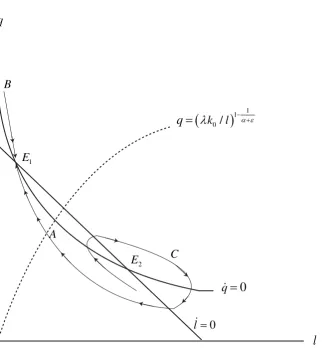
It is easy to con…rm the above proposition by depicting the phase diagrams of (30) and (31). Figures 1,2 and 3 display typical phase diagrams when there are dual steady state equilibria. First, we should con…rm that in these …gures, the stationary point with a lowerl

and a higherq (pointE1 in the …gures) attains a higher growth rate. To see this, …rst note

that from (34) the steady state level ofk increases with l:On the other hand (28) and (29) yield

v= x

k =

1

+" + (1 )

1 +"

kq 1+" 1:

Since 0 < +" < 1; the above means that a lower l and a higher q yield a lower v: As a result, the balanced growth rate,g= 1 l v ;attained at equilibriumE1 is higher

than that at E2 which associate with a higher l and a lower q: We see that (35) and (26)

respectively hold atE1 and E2:In addition, E2 is a sink under (37) and it is a source if (37)

does not hold.

In Figure 1, the steady-state with a lower growth rate is a source, so that there is no con-verging path aroundE2:Since E1 is a saddle point, there are two converging paths towards

E1:Given the initial level of capital ratio, k0;the economy’s initial position is on the doted

line that expresses equation (29). Hence, the initial levelsl and q are uniquely determined on the converging saddle path (point A in the …gure). If the economy starts from point A;

9_{Xie (1994) also conducts transitional analysis of the Lucas model with multiple equilibria. Since his model}

it converges monotonically towards E1: During the transition, l decreases and q increases

monotonically. Thus, as pointed out above,v also monotonically decreases in the transition process, which means that accumulation rate of human capital continues increasing. In con-trast, if the economy starts from pointB;thenlandqrespectively increases and decreases on the converging path. Hence, the accumulation rate of human capital monotonically decreases during the transition. The monotonic convergence, however, does not hold, if the economy starts from a point close toE2 (pointC;for example).

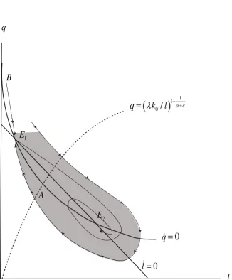
Figure 2 illustrates the case where the low growth steady state is a sink: there is a continuum of converging paths aroundE2: The phase diagram indicates that not only local

indeterminacy but also global indeterminacy can be observed in this case. If the initial level of k gives the doted line (equation (29)), any point between A and B would be a feasible initial position of the economy. For example, if point A is the initial point, the economy converges to the higher growth steady state monotonically. But the economy may leaves from point B towards E1: If this is the case, the converging process is not monotonic (the

growth rate of human capital …rst rises and then decreases during the transition towards pointE1):However, taking the starting position on pointAorBis almost coincidence, if the

initial position of the economy is randomly chosen: there are a continuum of feasible initial points on the line betweenA and B that lead the economy to the low growth steady state,

E2:Unless, the agents anticipate that their destiny will be the high growth steady state, the

economy almost always converges to the low growth steady state. In this sense, the dynamic system exhibits global indeterminacy as well as local indeterminacy.

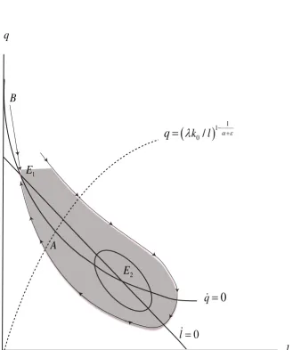
Such kind of global indeterminacy may emerge even though the low growth steady state is not locally indeterminate. In Figure 3, the low growth steady state,E2;is again assumed

to be totally unstable. Thus unless the initial position isE2 itself, any trajectory aroundE2

will diverge. We should notify that in this …gure one of the unstable saddle path diverging from the high growth steady state, E1;tends to converging to the low growth steady state.

However, sinceE2 is a source, the unstable saddle path cannot converges to E2:In addition,

we see that any path starting from in the shaded area will remain in this area. Consequently, in view of Poincaré-Bendixson theorem, there exists at least one stable limit cycle around

E2:In other words, any trajectory within the shaded area eventually converges to the stable

equilibrium with a higher growth rate or the cyclical growth path around the low growth steady state. Again, the dynamic system displays global indeterminacy.

4.2 Implications

The graphical analyses conducted above make three points. First, when there are dual steady states, two economies that have the identical technology and preference may display completely di¤erent growth performances even though they start with the same levels of physical and human capital. Additionally, even when the economy converges to the same steady state that is locally determinate, the convergence trajectory may not be monotonic. If the economy starts from the position such as PointAin Figure 1, the economy monotonically converges to the balanced-growth equilibrium as the standard Lucas model does. However, when the economy starts from Point C in Figure 1, the growth rate of human capital …rst decreases and then increases up to the higher balanced growth rate. Hence, when we focus on the determinate equilibrium, the long-term growth pattern would depend on the initial level of capital stocks. It is to be noted that this kind of non-monotonic converging behavior of human capital formation has already been pointed out by Xie (1994).

Second, in the case of dual steady states, the possibility of realization of the low-growth steady state is much higher than that of the high-growth steady state. This is because, if the low-growth steady state is locally indeterminate (or locally unstable but there exists a stable cycle around it) and if the initial position of the economy is randomly selected, the economy will almost always converges to the steady state with a lower growth rate. This means that the destiny of the economy can be the steady state with a higher growth rate only when the economic agents share an optimistic view about the future of their economy. In other words, the conventional growth promoting policies would not be enough to make the economy converge to the high growth steady state.

between volatility and growth is still a controversial issue in the empirical literature, our discussion suggests that the relation between growth and volatility would not be examined properly if the researchers presume that the fundamental shocks are only sources for economic ‡uctuations.

In his well cited essay on the growth miracle of East Asian countries, Lucas (1993) states that multiplicity of equilibrium may present a useful insight as to why the countries with similar economic conditions can display diverse growth performances in the long run. As a typical example, he mentions comparative growth performances between South Korea and Philippines. In the early 1960s, per-capita income of both countries were about the same. In addition, they shared many common features such as population size, degree of urbanization, rates of school enrollment and the like. After three decades, per-capita income of South Korea became more than three times as large as that of Philippines. If we stick to the idea that the economies with the same economic conditions must follow the same growth process, we should seek more fundamental di¤erences between South Korea and Philippines that eco-nomic theory usually dismisses, that is, the di¤erences in political stability, religion, climate, social atmosphere, so on. In contrast, if we consider the possibility of multiple equilibria, we may explain the reason of income divergence without considering those non-economic conditions. Obviously, we cannot claim that divergence of per-capita income between South Korea and Philippines has been generated by multiplicity of equilibrium alone. However, from the view point of economic theory, it is insightful to use the growth models with multi-ple equilibria when we explore the reasons as to why some East Asian countries have attained extremely good performances in growth but the countries in South Asia with similar economic fundamentals have shown relatively poor growth performances.

5

Concluding Remarks

global indeterminacy may emerge.

An obvious limitation of our discussion is that the main analytical results concerning global dynamics of the economy hinge on the particular speci…cation of the parameter values involved in the model. In particular, we have assumed that = ; which means that the interemporal elasticity of substitution in the felicity function,1= ;is close to 3.0 if we assume that the income share of physical capital, ; is around 0.35. Namely, establishing indeter-minacy under social constant returns requires that the preference structure satis…es strong convexity. The foregoing studies on indeterminacy in growth models have generally shown that there exists a trade-o¤ between nonconvexity of production technology and convexity of preferences to hold indeterminacy: in order to …nd out indeterminacy conditions, the model with convex technology tends to need strong convexity of preferences, while the models with weak convex preferences should assume the presence of strong non-convexity of technology. As emphasized earlier, our model is free from the criticism claiming that the growth models with indeterminacy of equilibrium should assume empirically implausible degree of increasing returns. On the other hand, the high degree of intertemporal substitutability of consumption assumed in our discussion would lack plausibility.10

We should, however, note that further generalization may weaken the restrictive assump-tions in our model. For example, it has been known that introducing distortional taxes on factor income or endogenizing capital utilization can substantially lower the required degree of increasing returns in the models with indeterminacy. Those kind of extensions would also be useful to hold indeterminacy in the model of constant returns with weaker restrictions on the parameter magnitudes. As stated in the introduction of the paper, our main purpose is to present an example demonstrating that complex dynamics may emerge in the standard mod-els with small modi…cations. Hence, to make such a claim more convincing, further extensions of the model seem to be necessary. This is a relevant topic in the future investigation.

1 0_{If we use a simpler models that does not involve physical capital, we may obtain the essentially the same}

conclusions shown in this paper without assuming that = : see Mino (1999a):Thus the main results in this

References

[1] Benhabib, J. and Farmer, R.E. (1994), ”Intermediacy and Growth”,Journal of Economic Theory 63, 19-41.

[2] Benhabib, J. and Perli, R. (1994), ”Uniqueness and Indeterminacy: Transitional Dy-namics”,Journal of Economic Theory 63, 113-142.

[3] Benhabib, J. and Farmer, R.E. (1996), ”Indeterminacy and Sector Speci…c Externali-ties”, Journal of Monetary Economics 37, 397-419.

[4] Benhabib, J. and Farmer, R.E. (1999), ”Indeterminacy and Sunspots in Macroeco-nomics”, inHandbook of MacroeconomicsVolume 1, edited by J.B.Taylor and M.. Wood-ford, North-Holland, 387-443.

[5] Benhabib, J., Meng. Q., and Nishimura, K. (1999), ”Indeterminacy under Constant Returns to Scale in Multisector Economies”, Econometrica 68, 1541-1548.

[6] Bennett, R.L. and Farmer, R.E. (1998), ”Indeterminacy with Nonseparable Utility”,

Journal of Economic Theory 93, 118-143.

[7] Boldrin, M. and Rustichini, A. (1994), ”Indeterminacy of Equilibria in Models with In…nitely-lived Agents and External E¤ects”, Econometrica 62, 323-342.

[8] Krugman, P. (1991), ”History versus Expectations”, Quarterly Journal of Economics

106, 651-667.

[9] Ladrón-de-Guevara, A., Ortigueira, S. and Santos, M. S. (1999), ”A Two-Sector Model of Endogenous Growth with Leisure”,Review of Economic Studies 66,609-631.

[10] Lucas, R.E., (1988), ”On the Mechanics of Development”, Journal of Monetary Eco-nomics 22, 3-42.

[11] Lucas, R.E., (1993), ”Making a Miracle”,Econometrica 42, 293-316.

[13] Mino, K. (1999a), ”Non Separable Utility Function and Indeterminacy of Equilibrium in a Model with Human Capital”, Economics Letters 62, 311-317.

[14] Mino, K. (1999b), ”Indeterminacy and Endogenous Growth with Social Constant Re-turns”, forthcoming inJournal of Economic Theory.

[15] Pelloni, A. and Waldman, R. (2000), ”Can West Improve Welfare?”,Journal of Public Economics 77, 45-79.

[16] Perli, R. (1998), ”Indeterminacy, Home Production and the Business Cycles: A Cali-brated Analysis”,Journal of Monetary Economics 41, 105-125.

[17] Romer, P.M. (1986), ”Increasing Returns and Long Run Growth”, Journal of Political Economy 94, 1002-1034.

Figure 1: The high growth equilibrium (point ) is a saddlepoint

and the low-growth equilibrium (point ) is a source.

E

2 E

0

q



0

l





q





q

l

A

C B

1 E

1

E

2

E

0

q





0

l









1 0

/

k

l

q





q

l

A

B

Figure 2

1

E

2

E

A

1

E

2

E

0

q





0

l









1 0

/

k

l

q





q

l

A

B

Figure 3

1

E

2

E

A