Data Revisions in India and its Implications for Monetary Policy

Munich Personal RePEc Archive

Data Revisions in India and its

Implications for Monetary Policy

Kishor, N. Kundan

University of Wisconsin-Milwaukee

July 2009

Online at

https://mpra.ub.uni-muenchen.de/16099/

Data Revisions in India and its Implications for

Monetary Policy

N. Kundan Kishor

University of Wisconsin-Milwaukee

Abstract

This paper studies data revision properties of GDP growth and in‡ation as mea-sured by the Wholesale Price Index (WPI) for the Indian economy. We …nd that data revisions to GDP growth and WPI in‡ation in India are signi…cant. The results show that revisions to GDP growth and WPI in‡ation can not be characterized as either containing pure news or pure noise. We also …nd that there is a signi…cant predictable component in revisions to GDP growth and in‡ation. Our …ndings suggest that if the Reserve Bank of India were to follow a Taylor rule for its monetary policy formulation, then the interest rate based on the preliminary data would be much lower than the one based on the fully revised data.

1

Introduction

Most of the macroeconomic time-series data are subject to revisions. Data revisions pose a

problem for policymakers since they formulate policies in real-time without access to the fully

revised data. It also causes problems for economic researchers since their empirical work is

based on heavily revised data, and the policy conclusions based on the use of heavily revised

data can often be misleading in real-time. Recently there has been a surge in literature on

data revisions and its implications for policy making1_{. Most research on data revisions has}

I am thankful to Mr. Ramesh Kolli of Central Statistical Organization, Government of India, for sharing the data on GDP releases.

y_{Department of Economics, Bolton Hall 806, University of Wisconsin-Milwaukee, WI-53201. E-mail:} [email protected].

been performed on OECD countries especially the U.S. economy. The issue of data revisions

in developing countries has not attracted a great deal of attention due to lack of real-time

data2_.

The macroeconomic time-series data in India are also subject to revisions. GDP growth

and the Wholesale Price Index (WPI)- the primary measure of in‡ation in India- undergo

heavy revisions. Figures 1 and 2 plot revisions to GDP growth and aggregate in‡ation in

India. It is evident from the graph that the …nal estimate of in‡ation is higher than the

preliminary estimate for the larger part of the sample since revisions are almost always

positive. The revisions to GDP growth show higher volatility before 2001, and has been

mostly positive though less volatile since then.

This paper studies the data revision properties of GDP growth and the WPI in‡ation

and its sub-components in India, namely, primary, manufacturing, and fuel in‡ation3_{. We}

examine whether data revisions to GDP growth and in‡ation have zero mean, and whether

it can be forecasted using the information available at the time of the preliminary data

an-nouncement. This …ts in with the news versus noise literature in the data revision that has

been studied extensively for the key macroeconomic variables in the U.S.4_{. Conventional}

wisdom also suggests that data revisions pose a serious problem for monetary policy

formu-lation, as the monetary policy makers are uncertain about the true state of the economy on

the basis of preliminary estimate of macroeconomic variables. We also examine the e¤ect

of data revisions on monetary policy formulation in India. Speci…cally, we examine how the

interest rate prescribed by a Taylor rule would di¤er if real-time data is used instead of the

fully revised data.

Literature on data revisions has become quite extensive after compilation of the

real-time data set at the Federal Reserve Bank of Philadelphia by Croushore and Stark (2001).

Croushore and Stark (2001) show that the data revisions pose a serious challenge for policy

2_{Notable exceptions are Urdaneta (1974), Van de Eng (1999), Chumacero and Gallego (2001) and Palis}

et al. (2003)

formulation as well as the econometric estimation of the macroeconomic models. A big

part of the literature on data revisions investigate the revision properties, and tests whether

these revisions are predictable or not. Mankiw et al. (1984) tests whether preliminary

announcement of money stock are rational forecasts of …nal announcements. Mankiw and

Shapiro (1986) applied the similar analysis to GNP data. Faust et al. (2005) tested the

news versus noise hypothesis for revisions to the OECD output data, and found evidence

in support of the noise hypothesis. Croushore (2008) studied the patterns of data revisions

to the in‡ation rate in the U.S., and found that it is possible to forecast revisions from the

initial release. He noted that the initial release of in‡ation is likely to be revised up, as the

initial release is usually too low.

We …nd that revisions to GDP growth between 1997 and 2001 are characterized by

two regimes: volatile and insigni…cant revisions between 1997-2001:Q1 and mostly positive

and signi…cant revisions after 2001:Q1. The revisions to GDP growth after 2001 are also

associated with lower volatility. Data revisions to in‡ation in India are always signi…cant.

Speci…cally, we …nd that revisions to the WPI in‡ation and its sub-components are likely to

be revised up, as the preliminary estimates are too low. This e¤ect is especially pronounced

for manufacturing in‡ation which accounts for the biggest share of aggregate in‡ation.

Our results show that the data revisions to output growth and in‡ation in India can not

be strictly characterized as either containing pure news or pure noise. There is evidence of

predictability in data revisions using the preliminary announcement. We …nd that 39

per-cent of the variation in the data revisions to GDP growth between 1997:Q2-2001:Q1 can be

explained using preliminary release of GDP growth, whereas the corresponding explanatory

power of the initial release is 22 percent after 2001:Q1. Around 17 percent of the variation

in data revision to aggregate in‡ation can be explained by the initial release of the in‡ation.

The degree of predictability is greater for revisions to the manufacturing component of

in-‡ation as compared to the fuel and light, and the primary products. Around 39 percent of

the variations in revisions to manufacturing in‡ation can be explained using the preliminary

con-sistent with the late arrival of source data for the manufacturing component of the WPI.

The rejection of the pure news and the pure noise hypothesis is consistent with what has

been found by Mork (1987), and Aruoba (2008) for most of the U.S. macroeconomic time

series data. The ex-post predictability of data revision does not imply that data revisions

are forecastable in real-time. To investigate the real time predictability of data revisions, we

compare the forecast error of revision forecast generated in real-time with the actual revision

(assuming preliminary data as forecast of the …nal data), and we …nd that revision forecasts

can be substantially improved upon in real-time.

Our results show that ignoring data revision can have serious implications for monetary

policy formulation. We …nd that if the Reserve Bank of India were to follow the Taylor

rule in setting the interest rate, then the interest rate based on heavily revised data is

signi…cantly di¤erent than the one based on real-time data. The Taylor interest rates based

on the preliminary data tends to be usually too low. This implies that if the Reserve Bank

of India does not take into account the data revision that could take place in future, then

the monetary policy action may turn out to be too expansionary ex-post.

The plan of the remainder of this paper is as follows. Section 2 discusses the data

and its properties. Section 3 reviews the standard models of revision process and presents

the empirical results. Section 4 assesses the impact of data revisions on monetary policy

formulation in India and section 5 summarizes the main results.

2

Data Description

2.1

GDP Growth

The quarterly estimates of the GDP in India were introduced in 1999 beginning with the

year 1996-975_{. The quarterly GDP estimates once released are not revised till the release of}

Q4 estimates of GDP. This implies that the GDP growth rates of Q1, Q2 and Q3 are revised

only at the time of releasing the fourth quarter GDP estimates.

5_{The …scal year in India runs from April to March. Hence 1996-97 implies April 1996 to March 1997. Q1}

The revisions to the GDP growth are performed annually6_{. The Advanced Estimates}

of annual national income are released two months before the close of the year. These

advanced estimates are subsequently revised and released alongwith 4th quarterly estimates

of GDP, on the last working day of June, i.e. with a lag of 3 months. The Quick Estimates

are released in the month of January of the following year with 10 months lag. Alongwith

the Quick Estimates, the estimates for the previous years are also revised and released

simultaneously. The quarterly estimates are also revised alongwith the annual estimates in

January. Revisions in GDP growth rates take place over a period of four years with the …rst

revision termed as Quick Estimates. All these revisions take place annually, at the end of

January.

In this paper, we focus on the …rst release and the current estimate of the GDP growth.

Ideally, it would have been more interesting to examine the data revision properties of

di¤erent vintages of output growth, however, we are constrained by data availability and

focus on the …nal revisions in this paper.

2.2

In‡ation

Three di¤erent price indices are published in India: the Wholesale Price Index (WPI), the

Consumer Price Index (CPI), and the GDP de‡ator. The CPI has di¤erent classi…cations:

CPI for industrial workers, CPI for urban non-manual employees, and the CPI for the rural

sector. The WPI is a weekly series announced every Thursday, the CPI is a monthly index

and is made available with a lag of about one month, while GDP de‡ator data are available

annually.

The WPI is the most comprehensive measure of prices in India, and is used widely for

policy deliberations7_{.. The Reserve Bank of India (RBI) also cites WPI movements in every}

policy draft. The WPI covers 447 commodities and is heavily weighted towards manufactured

products. The WPI has three main sub-components: primary product, fuel, power and light,

and manufacturing products. Primary products mainly include food products. The current

weights of these three components in the calculation of the WPI are 22%, 14% and 64%

respectively. The WPI represents the quoted price of bulk transaction generally at primary

stage. It di¤ers from producer prices as the latter excludes all kind of taxes and transport

charges8_.

The …rst release of the WPI is provisional with a two week lag. There is only one round

of revision and the …nal index is released after a gap of eight weeks. The di¤erence between

provisional and the …nal index is mainly due to the poor response from the manufacturing

sector. The Department of Industrial Policy and Promotion (DIPP) is able to collect only

20 per cent of the data sought from the manufacturing sector when the …rst numbers are

released. But when the …nal numbers are released, the response increases to 65 per cent.

There is an almost 100 per cent reporting in primary goods when the …nal numbers are

released.

Our sample period runs through 1998:Q2 to 2008:Q4. The quarterly estimate of WPI

is calculated using the average of the weekly estimates of WPI, and the in‡ation rate is

the quarterly changes in the price level. These quarterly changes are in percentage terms

and annualized. The sample size is constrained by the availability of the data set on the

Reserve Bank of India’s website. Unlike the U.S., there is no central database for real-time

data in India. We gather provisional data on WPI and its sub-components from the weekly

statistical supplement (WSS) published by the Reserve Bank of India. The supplement also

publishes data on the di¤erent components of WPI.

3

Forecastability of Data Revisions

3.1

Bias in Revisions and Other Summary Statistics

Table 1 shows the summary statistics of revisions to GDP growth. While we …nd that

revi-sions are insigni…cant for the whole sample, the graph of revirevi-sions in …gure 1 indicates that

the period prior to 2001 is characterized by huge swings in revisions. We suspect that the

huge revisions prior to 2001 may disproportionately a¤ect the results for the whole sample.

Therefore we divide the sample into pre-2001:Q1 and 2001:Q1-2008:Q4 subperiods9_{. Our}

…ndings suggest that revisions are highly variable though insigni…cant in the …rst subsample

with maximum revision at 3.6 percent and minimum at -2 percent. The mean revision after

2001 has been larger and signi…cant at 10 percent. We use Newey-West (1987)

heteroskedas-ticity and autocorrelation consistent errors to test for the signi…cance of data revisions.

Table 2 reports summary statistics of data revisions to in‡ation and its sub-components

for the Indian economy. The results indicate that revisions are quite large and positive for

all variables. Among the sub-components of in‡ation, fuel component has the highest mean

revision, though the standard deviation of revision is also very high. The revisions to in‡ation

and its sub-components are signi…cant, as t-statistics are greater than two for the null of

mean revision equal to zero. The t-stat is based on Newey-West (1987) heteroskedasticity

and autocorrelation consistent errors. The interpretation of this result is that the initial

announcements of the statistical agencies are biased estimates of the …nal values. On average

the preliminary in‡ation is revised upwards with the mean annualized revision around 1.3

percent for the aggregate in‡ation. Table 2 also reports the minimum and the maximum

revisions for di¤erent components of in‡ation. The range of revisions are quite large for

in‡ation and its sub-components. The revision variability is highest for fuel followed by

primary components. We …nd that the range of revisions to manufacturing is small relative

to the other sub-components, and similar to the overall in‡ation. This is not surprising

since manufacturing accounts for two-thirds of the overall WPI in India. Hence, our results

indicate that revisions to in‡ation are signi…cant and positive, and the …nal estimate of

in‡ation is usually larger than the preliminary estimate.

3.2

Data Revisions: News or Noise

There are two extreme cases of data revision characterized by either containing news or noise

according to Mankiw, Runkle, and Shapiro (1984) and Mankiw and Shapiro (1986). Under

the news view, a statistical agency optimally uses all the available information in

announc-ing the preliminary data and revisions must re‡ect news that arrive after the preliminary

announcement. Therefore revisions must be orthogonal to all the available information at

that time. Under the noise characterization, the preliminary announcement is a noisy

mea-sure of the …nal announcement and this noise gets reduced after rounds of revisions. These

two types of data revision properties have implications for the standard error of preliminary

data and the …nal release of data. The standard error of preliminary release data is higher

than that of the …nal release under noise hypothesis, whereas the standard error of the …nal

release is higher than the preliminary release if the data revisions are characterized as news.

Formally speaking, if ypt is the preliminary estimate of variable yt and y f

t is the …nal

estimate, then we can characterize the preliminary data as equal to the …nal plus an error

term:

ypt =y f

t +"t (1)

If the noise model is correct, then the error term is orthogonal to ytf; whereas the error

term is orthogonal to the preliminary data if the news hypothesis is correct. In a regression

framework, Mankiw et al. (1984) considered the following framework:

ypt = 1+ 1y

f t +"

1

t (2)

yft = 2+ 2y

p t +"

2

t (3)

where the noise hypothesis implies testing a joint hypothesis of 1 = 0; 1 = 1;while a joint

hypothesis of 2 = 0; 2 = 1tests the news hypothesis. As argued by Aruoba (2008), these

two hypotheses are mutually exclusive but are not collectively exhaustive, that is, we can

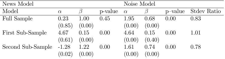
Table 3 reports the estimate of news versus noise model for GDP growth. The results

show that except for the news model for the whole sample, we reject the null of news as

well as the noise model for all sample periods. P-value in the table is the P-value for a null

hypothesis of i = 0; i = 1; i= 1;2:We observe a signi…cant di¤erence in the estimate of

and for di¤erent subsamples. The constant term is relatively large for the …rst subsample,

whereas the coe¢cient on the preliminary estimate for the news model and the …nal estimate

for the noise model is insigni…cant. This implies that revisions are on average large though

highly volatile. The results for the second subsample also rejects both the news and the

noise hypothesis. In both models, signi…cant unconditional mean is the main source of the

rejection of both hypotheses.

Table 4 reports the results for news versus noise test for aggregate in‡ation and its

sub-components. The results indicate that both the news and the noise hypotheses are rejected at

10% signi…cance level for all variables. Among the sub-components of WPI, manufacturing

provides the strongest evidence against both hypotheses. When we investigate the source of

the rejection of both hypotheses, we …nd that the constant is signi…cantly zero in all cases,

and the slope coe¢cient is statistically di¤erent from zero for manufacturing and aggregate

in‡ation. This implies that the positive unconditional mean of revisions is the main source

of the rejection of the news and the noise hypotheses.

Therefore our results suggest that revisions to GDP growth and in‡ation in India can

not be characterized as optimal forecast error or measurement error. The results obtained

here is consistent with what Mork (1987) and Aruoba (2008) found for the U.S. data.

3.3

Ex-Post Forecastability of Data Revisions

The results presented in the previous section suggest that data revisions to GDP growth

and in‡ation in India can not be characterized as either containing pure news or pure noise.

Rejection of pure news hypothesis implies that there is some degree of forecastability present

in the data revision. If revisions are not forecastable, then the conditional mean of revision

To test the degree of forecastability present in the revision process, we run the following

baseline regression:

rt= + ytp+vt (4)

where rt is the di¤erence between the …rst release and the …nal estimate of GDP growth and

in‡ation10_{. We test for joint hypothesis of = = 0: This equation can also be augmented}

by including the variables known at time t11_{. This test of ex-post forecastability of data}

revisions is sometimes called the Mincer-Zarnowitz test.

Table 5 presents estimation results for output growth. The results are consistent with

the rejection of the news hypothesis in the previous section. We …nd that revisions to GDP

growth for the whole sample can not be predicted using the preliminary estimate12_{. However,}

there is strong evidence of predictability in revisions when we perform the same analysis

for di¤erent subsamples. The results imply that the coe¢cient on the explanatory variable

cancels each other out when the whole sample is taken into account. Surprisingly, the results

for the sample period before 2001:01 show that a percentage increase in the growth rate of

preliminary estimate of real GDP leads to a downward revision of 0.85 percent. Thirty two

percent of the variations to revisions in the …rst subsample is explained by the preliminary

estimate. Our results show that around 22 percent of the variations in revisions after 2001:02

are explained by the preliminary estimate. The estimated results indicate that a percentage

increase in preliminary estimate of GDP growth leads to a 0.22 percent increase in revisions.

For in‡ation, the results indicate that the preliminary announcement of WPI and its

components help in predicting subsequent revisions in 3 out of 4 cases. The degree of

predictability varies across di¤erent components. The results show that preliminary measure

of manufacturing in‡ation explains 39% of the variations in subsequent revisions, whereas

the preliminary measure of the aggregate in‡ation explains 17% of the variation in revisions.

10_{The test of forecastability is very similar to testing for the news hypothesis.}

11_{Similar tests have been performed by several researchers for the U.S. data, examples include Faust et al.}

(2005), Kavajecz and Collins (1995), Aruouba (2008), Croushore (2008).

12_{We test for the stability of equation (4) using Andrews-Ploberger test, and …nd that the null of no}

For revisions to primary goods in‡ation, 10 percent of its variations can be explained by

its preliminary measure. Our results show that preliminary estimate explains 7 percent

of the variations in revisions to fuel in‡ation. Overall, results indicate that preliminary

announcement of di¤erent components of in‡ation can be used to predict the subsequent

revisions, though the degree of predictability di¤ers for di¤erent components of in‡ation.

3.4

A Real-Time Forecasting Exercise For In‡ation

The forecastability result obtained above does not imply that the data revisions are

fore-castable in real-time. The estimation results can only be observed after the fact from the

complete sample. We use the full sample information to estimate equation (4), whereas a

forecaster in real-time does not have the access to the future data. For example, if one’s goal

in 1999:Q2 is to forecast the data revisions in future, one is constrained by the availability

of data in1999:Q2 and hence can not use the future data.

Since we are constrained by the availability of di¤erent vintages of data for the GDP

growth, we focus on forecasting revisions to in‡ation in time. To investigate the

real-time predictability of data revisions in in‡ation in India, we perform the following recursive

exercise. The …rst step, using t+1 vintage data is to run the following regression:

r(t; t+ 1) = + ytp+vt (5)

where r(t; t+ 1) is the revision of period-t in‡ation that becomes available at t+1. Since

we are using quarterly data, and there is a lag of one period in the announcement of the

…nal data, the …nal estimate of period-t in‡ation and the preliminary estimate of period-t+1

in‡ation are available at t+1. Therefore using the information available at time t+1, we run

a simple OLS regression of the revision on its preliminary estimate ytp: Using the estimated

value of and ;and the preliminary estimateypt+1;which is available at t+1, we predict the

revision of period-t+1 in‡ation r(t+ 1; t+ 2). In the second step, we calculate the forecast

of the …nal estimate of in‡ation by adding the revision to the preliminary estimate, and

procedure is repeated for every new release from 2002:Q2 to 2008:Q4. Total number of

forecasts for this exercise turns out be 41. This recursive forecasting exercise provides us the

real-time forecasts of revisions.

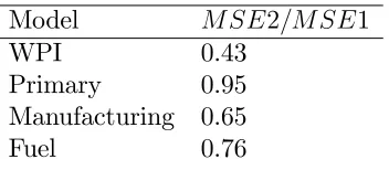
Table 7 reports the ratio of mean squared errors (MSE) of the real-time forecasts

gen-erated from the above methodology and mean squared error computed with preliminary

data as the forecast of the …nal estimate of in‡ation. The ratio below unity represents a

superior forecasting performance of the real-time recursive forecast. The results in table 4

indicate that except for fuel component of WPI in‡ation, we are able to reduce the MSE of

the revision forecasts in real-time signi…cantly. The degree of reduction in MSE is highest

for the manufacturing component, which is not surprising since the preliminary

announce-ment of manufacturing in‡ation explains 35 percent of the variation in revisions ex-post.

We do not observe a big improvement in the forecast of fuel in‡ation, which is consistent

with Mincer-Zarnowitz test results. The improvement in forecasting performance is driven

by the biasedness and the predictability of data revisions. Our examination of the property

of data revisions in previous sections shows that revisions to in‡ation are not insigni…cant,

in fact, they are large and signi…cant for aggregate and manufacturing in‡ation. Similarly,

we …nd that a signi…cant portion of the variation in revisions to in‡ation can be explained

using the preliminary announcement. The results obtained in this section indicate that we

can use preliminary data to predict data revisions in real-time, and the improvement can be

substantial for aggregate and manufacturing in‡ation.

4

Impact of Data Revisions on Monetary Policy

For-mulation

The results obtained in the previous section suggest that the GDP growth and in‡ation

undergo signi…cant revisions. As a result, it is possible that the monetary policy that may

seem appropriate in real-time may turn out to be either too tight or too loose. To investigate

the potential impact of data revisions on monetary policy in India, we perform a very simple

as well as the fully revised data. In doing so, we do not intend to evaluate the actual impact

of data revisions on the monetary policy actions of the Reserve Bank of India. Our simple

goal is to examine the di¤erences in the interest rates suggested by Taylor rule that could

arise as a result of data revisions.

We follow Taylor (1993) in computing the appropriate interest rate, which is based on

in‡ation and output gap. Taylor (1993) considers a representative policy rule which looks

like:

rt= +:5y+:5( 2) + 2 (6)

where rtis the federal funds rate implied by Taylor rule, is the rate of in‡ation, y is output

gap. We calculate …rst release and current vintage output gap using Christiano-Fitzgrald

asymmetric …lter1314_.

The interest rates based on the …rst release and the latest vintage data of in‡ation and

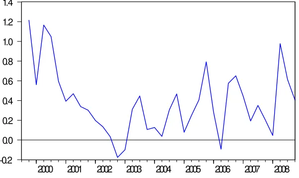
output gap are shown in …gure 3. It is evident from the graph that the interest rate based on

fully revised data is higher on average than the interest rate based on …rst release data. This

is not surprising since our previous results show that in‡ation is most likely to be revised up

after the …rst release. To make the comparison between interest rates of these two vintages,

we also plot the di¤erence between the interest rate based on fully revised data and the …rst

release data. As shown in …gure 4, except for a short span in 2002 and 2006, the di¤erence

is always positive. In fact, the mean of the di¤erence between the interest rates is 40 basis

points and it is signi…cant15_{. The results imply that if monetary policy is based on the …rst}

release data, then according to the Taylor rule, the interest rates will be too loose and may

in‡ate the economy.

13_{The results are qualitatively similar if we use HP …lter.}

14_{We are also aware of the problems associated with estimation of output gap, especially in a developing}

country like India, however, the purpose of this exercise is not to estimate output gap but to assess the impact of data revisions on monetary policy. As long as estimated output gaps based on di¤erent methods do not move in opposite direction, the results obtained will be qualitatively similar.

15_{To test the signi…cance of the di¤erence beween interest rates, we regress the di¤erence on a constant.}

5

Concluding Remarks

This paper studies the data revision properties of GDP growth and in‡ation and its

implications for monetary policy formulation in the Indian economy. While the GDP

un-dergoes multiple rounds of revisions, WPI which is the primary measure of prices in India,

and is used widely for policy deliberations undergoes one round of revision with a lag of

eight weeks. We …nd that revisions to WPI in‡ation and its sub-components are positive

and signi…cant. The results indicate that on average the …nal estimate of in‡ation is higher

than the preliminary estimate, and is likely to be revised up. The revisions to GDP growth

were volatile and insigni…cant before 2001, but positive and signi…cant after 2001.

Our results show that the data revisions to GDP growth and WPI in‡ation and its

sub-components can not be characterized as either containing pure news or pure noise. We …nd

that the use of preliminary data can signi…cantly improve the naive zero-forecast, which

would be optimal if the preliminary announcements are the optimal forecasts of the …nal

values. This holds for both in an ex-post forecasting exercise, as well as real-time forecasting

exercise for in‡ation.

Our results indicate that around 22 percent of the variations in revisions to output growth

after 2001:Q1 can be explained using the preliminary estimate of GDP growth, whereas the

corresponding number for aggregate in‡ation is 17 percent. The degree of predictability

for data revisions to manufacturing in‡ation is higher than the other sub-components of

in‡ation. We …nd that 39 percent of the variations in revisions to manufacturing in‡ation

can be explained using the …rst release.

The results obtained in this paper suggest that ignoring data revisions in GDP growth

and WPI in‡ation can have signi…cant policy consequences. If the Reserve Bank of India

were to follow a Taylor rule in monetary policy formulation, then our results indicate that

monetary policy based on preliminary data is too expansionary ex-post. More speci…cally,

interest rates based on preliminary data turns out to be lower than the interest rates based

References

[1] Aruoba, S. Boragan (2008),“Data Revisions are not Well Behaved, ”Journal of Money,

Credit and Banking, 40, pp. 319-340.

[2] Business Standard (2008), “Final Estimate of WPI Good Enough,” August 23.

[3] Chumacero, R. A., and Gallego, F.A., (2001), “ Trends and Cycles in Real-Time,”

Central Bank of Chile Working Paper No. 130.

[4] Croushore, Dean and Tom Stark (2001), “A Real-Time Data Set for Macroeconomists,”

Journal of Econometrics, 105, pp. 111-130.

[5] Croushore, Dean (2008a), “Revisions to PCE In‡ation Measures: Implications for

Mon-etary Policy,” Federal Reserve Bank of Philadelphia Working Paper.

[6] Croushore, Dean (2008b), “Frontiers of Real-Time Data Analysis,” Working Paper.

[7] Faust, Jon, John H. Rogers, and Jonathan H. Martin (2005), “News and Noise in G-7

GDP Announcements,” Journal of Money, Credit and Banking, 37, pp. 403-419.

[8] Government of India, Ministry of Commerce and Industry (2009), “Manual:

Compila-tion of WPI,”.

[9] Kavajecz, K.A. and S. Collins (1995), “Rationality of Preliminary Money Stock

Esti-mates,” Review of Economics and Statistics, 77, pp. 32-41

[10] Kolli, Ramesh (2004), “ Revisions in India’s GDP Estimates,” OECD/ONS Workshop

on Assessing and Improving Statistical Quality, October 2004.

[11] Mankiw, N. Gregory, and Matthew D. Shapiro (1986), “News or Noise: An Analysis of

[12] Mankiw, N. Gregory, David E. Runkle, and Matthew D. Shapiro (1984), “ Are

Prelim-inary Announcements of the Money Stock Rational Forecasts?,” Journal of Monetary

Economics, 14, pp. 15-27.

[13] Mork, Knut A. (1987), “Ain’t Behavin’: Forecast Errors and Measurement Errors in

Early GNP Estimates,” Journal of Business and Economic Statistics, 5, pp. 165-175.

[14] Newey, W. and K. West (1987), “A Simple Positive Semi-De…nite, Heteroskedasticity

and Autocorrelation Consistent Covariance Matrix,” Econometrica, 55, 703-708.

[15] Palis, Rebeca de la Rocque, Roberto Luis Olinto Ramos, and Patrice Robitaille (2004),

“News or Noise? An Analysis of Brazilian GDP Announcements,” International Finance

Discussion Papers, Federal Reserve Board.

[16] Reserve Bank of India Weekly Statistical Supplements.

[17] Taylor, J.B. (1993), “ Discretion versus Policy Rules in Practice,” Carnegie-Rochester

Series on Public Policy, 23, pp. 194-214.

[18] Urdaneta, L. (1976), “Some Aspects of the Revision of the System of National Accounts

in Venezuela,” Review of Income and Wealth, v. 22, iss. 1, pp. 37-47.

[19] Van de Eng, P.(1999), “ Some Obscurities in Indonesia’s New National Accounts,”

Figure 1: Revisions to GDP Growth

-3 -2 -1 0 1 2 3 4

97 98 99 00 01 02 03 04 05 06 07 08

REV_GDP

Figure 2: Revisions to WPI In‡ation

-1 0 1 2 3 4

99 00 01 02 03 04 05 06 07 08

Figure 3: Interest Rates Based on Taylor Rule for Preliminary and Heavily Revised Data

0 4 8 12 16 20

2000 2001 2002 2003 2004 2005 2006 2007 2008

Taylor_Prelim Taylor_Current

Figure 4: Di¤erence in the Interest Rates Based on Taylor Rule for Preliminary and Heavily Revised Data

-0.2 0.0 0.2 0.4 0.6 0.8 1.0 1.2 1.4

Table 1: Summary Statistics of Revisions to GDP Growth

Model Mean Minimum Maximum Std Dev t-stat

Full Sample (1997:02-2008:04) 0.23 -2 3.6 1.26 1.16 First Sub-Sample (1997:02-2001:01) 0.01 -2 3.6 1.89 0.03 Second Sub-Sample (2001:02-2008:04) 0.35 -1.2 2.1 0.78 1.70

a

Revision is …nal minus preliminary estimate. The t-stat is based on autocorrelation and heteroskedastic consistent errors and

are for the hypothesis that the mean of the revision is zero.

Table 2: Summary Statistics of Revisions to In‡ation

Model Mean Minimum Maximum Std Dev t-stat

WPI 0.89 -0.84 3.19 0.78 6.22

Primary 0.50 -2.63 6.73 1.82 1.95 Manufacturing 0.97 -1.41 3.10 0.83 6.29

Fuel 1.13 -7.48 14.42 3.22 1.83

a

The …nal and the preliminary numbers are calculated as quarterly changes in the price level, and is annualized. Revision is

…nal minus preliminary estimate. The t-stat is based on autocorrelation and heteroskedastic consistent errors and are for the

hypothesis that the mean of the revision is zero.

Table 3: News versus Noise Model (Output Growth)

News Model Noise Model

Model p-value p–value Stdev Ratio

Full Sample 0.23 1.00 0.45 1.95 0.68 0.00 0.83 (0.85) (0.00) (0.00) (0.00)

First Sub-Sample 4.67 0.15 0.00 4.64 0.15 0.00 1.01 (0.61) (0.00) (0.00) (0.40)

Second Sub-Sample -1.28 1.22 0.00 1.61 0.74 0.00 0.78 (0.02) (0.00) (0.00) (0.00)

a

Table 4: News versus Noise Model (In‡ation)

News Model Noise Model

Model p-value p–value Stdev Ratio

WPI 0.56 1.07 0.00 -0.42 0.91 0.00 0.86 (0.00) (0.00) (0.02) (0.00)

Primary 0.10 1.09 0.02 0.11 0.88 0.00 0.88 (0.61) (0.00) (0.41) (0.00)

Manufacturing 0.45 1.16 0.00 -0.29 0.84 0.00 0.77 (0.00) (0.00) (0.00) (0.00)

Fuel 1.91 0.90 0.07 -1.15 1.00 0.15 0.95 (0.02) (0.00) (0.10) (0.00)

a

P-values are in parentheses. Newey-West heteroscedastic errors are used in estimation.

Table 5: Mincer-Zarnowitz Test (Output Growth)

Model p-value R2

SerialCorrelation

Full Sample (1997:02-2008:04) 0.23 0.01 0.45 0.00 0.21 (0.85) (0.99) (0.10) First Sub-Sample (1997:02-2001:01) 4.67 -0.85 0.00 0.39 0.16

(0.61) (0.00) (0.00) Second Sub-Sample (2001:02-2008:04) -1.27 0.22 0.00 0.22 0.30

(0.00) (0.00) (0.00)

a

Table 6: Mincer-Zarnowitz Test (In‡ation)

Model p-value R2

SerialCorrelation

WPI 0.56 0.08 0.00 0.17 0.24 (0.00) (0.00) (0.10) Primary 0.10 0.09 0.02 0.10 0.05

(0.61) (0.00) (0.00) Manufacturing 0.45 0.16 0.00 0.39 0.28

(0.00) (0.00) (0.00) Fuel 1.91 -0.09 0.07 0.08 0.37

(0.02) (0.04) (0.18)

a

P-values are in parentheses. Newey-West heteroscedastic errors are used in estimation.

Table 7: Real-Time Forecasting Performance

Model M SE2=M SE1

WPI 0.43

Primary 0.95 Manufacturing 0.65

Fuel 0.76

a

MSE1 is the mean squared error when the preliminary data is the forecast of the …nal data. MSE2 is the mean squared error