A NEW REAL CODED GENETIC ALGORITHM CROSSOVER:
RAYLEIGH CROSSOVER
*1SIEW MOOI LIM, 2MD. NASIR SULAIMAN, 3ABU BAKAR MD. SULTAN, 4NORWATI
MUSTAPHA, 5BIMO ARIO TEJO
1,2,3,4 Faculty Of Computer Science And Information Technology, Universiti Putra Malaysia, Malaysia
5 Centre For Infectious Diseases Research, Surya University, Indonesia
E-mail:*[email protected] & (2nasir, 3abakar, 4norwati)@fsktm.upm.edu.my & [email protected]
* Corresponding author
ABSTRACT
This paper presents a comparison in the performance analysis between a newly developed crossover operator called Rayleigh Crossover (RX) and an existing crossover operator called Laplace Crossover (LX). Coherent to the previously defined Scaled Truncated Pareto Mutation (STPM) operator to form two (2) generational RCGAs called RX-STPM and LX-STPM, both crossovers are utilized. A set of ten (10) benchmark global optimization test problems is used to investigate the reliability, efficiency, accuracy and quality of solutions of both optimization algorithms. Based on computational results, the RX-STPM has yield a significant better performance as compared to LX-STPM.
Keywords: Genetic Algorithms, Mutation Operator, Crossover Operator, Global Optimization
1. INTRODUCTION
Many real life problems in engineering, economics and science are modeled as a global optimization problems and this study seeks to find the set of variables that achieves the best possible value of the objective, among all those values that satisfy the constraints. Among the two major categories of global optimization algorithms are deterministic and stochastic approaches. The deterministic techniques obtain an approximate global minimum to the given accuracy. Stochastic techniques involved random search procedure, and it only offers a guarantee in probability and has no means to estimate the accuracy of the results obtained. As reported in the literature, stochastic techniques have satisfactorily provided answers to various problems. It is also the preferred algorithms when the size of the search space grows exponentially and other exact methods and effective algorithms are incapable of finding an optimal solution [1].
Evolutionary algorithm (EA) is a stochastic
search algorithm and a general-purpose
optimization method. Genetic algorithms (GA) [2], evolutionary programming [3] and evolutionary
strategies [4] are the three (3) parent methods of EA. These methods are based on the basic principles of Darwinian evolution, but they have
different strategies of computational
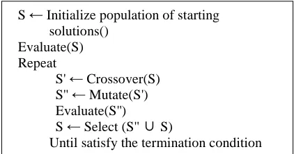
[image:1.612.314.525.491.602.2]implementation of these evolutionary principles [5]. Figure 1 shows the general scheme for EAs.
S ← Initialize population of starting
solutions() Evaluate(S) Repeat
S' ← Crossover(S)
S'' ← Mutate(S')
Evaluate(S'') S ← Select (S'' S) ∪
Until satisfy the termination condition
Figure 1: Basic Common Structure Used By EAs For Problem Solving
The GA is a generic adaptive strategy and a widely used optimization procedures [6]. Similar
to the Mendelian understanding of the
chromosomes, genes and alleles structure, GAs are moved by population genetics and evolution at the
population level. GAs mechanisms are
reproduction, crossover and mutation on
contributes their genotype to their suitability of their expressed phenotype in the form of offspring. The next generation is produced through a process of mating whereby the crossover operator takes two genotypes and combines them to form a new one either by merging or by exchanging the values of the genes. The mutation operator subsequently modifies one or multiple genes. This repeated process will develop an adaptive-fit between the phenotypes of individuals in a population.
GAs is typically represented in binary encodings. Having said that, the binary genetic representation does have its drawbacks [7]. Real encoding of chromosomes representations are developed to overcome the limitations of binary encoding. GAs which using the real number vector representation of chromosomes are termed as Real Coded GA (RCGA). There are many advantages of RCGAs over binary encoding GAs in numerical function optimization. Among them are that the conversion of chromosomes to the binary type is unnecessary hence efficiency of the GA escalates;
efficient floating-point internal computer
representations can be used directly thus memory prerequisite is lower; there is no loss in precision by discretisation to binary or other values; freedom to choose different genetic operators [8]. Herrera and Ono et al [9, 10] testified in recent years that RCGA has proven to outperform traditional bit
string based representation for function
optimization. Therefore, RCGA is endorsed for optimization problems where the parameter space is
continuous; it is also being pervasively
implemented in a wide range of applications [11].
The objective of the present study is to introduce a newly designed crossover operator called Rayleigh Crossover which uses Rayleigh Distribution. The subsequent section encompasses the literature review on real coded crossover operators. Section 3 defines the proposed RX and other operators used in this study. Section 4 involves a thorough discussion about the proposed new RCGAs. Section 5 deliberates the experimental setup while Section 6 discusses and explains the results. Section 7 reaffirms previous notions with a conclusion. Appendix A provides the 10 benchmarking functions.
2. LITERATURE REVIEW ON CROSSOVER OPERATORS
The key search operator in GA is the crossover operator. It is used to exploit the available
information from the population about the search space and thus improve the behavior of the GA. Efforts of the RCGA are channeled toward designing new crossover operators to heighten the
performance of function optimization [12].
Different operation of different crossover operators according to the literature is deliberated as follows:
Single point crossover [2, 13]: This operator
randomly identify one crossover point, then split parents at this crossover point and create children by exchanging tails. The typical crossover probability is in the range of 0.6 - 0.9. n-point
crossover [14]: This operator is a generalization of
the single point crossover. Randomly identify n crossover points. Then split along those points and glue parts then alternating between parents.
Uniform crossover [15]: This operator assigns
'heads' to one parent, 'tails' to the other. Then flip a coin for each gene of the first child and make an inverse copy of the gene for the second child. Inheritance is independent of position. Single
point, n-point and uniform crossover operators have
been used on binary and real-coded GAs.
Arithmetical crossover [11]: Some arithmetic
operations are performed to make a new offspring.
Flat crossover (BLX-0.0)[16]: Offspring was
generated randomly between the genes of the parents.
The five (5) operators mentioned above were among the first attempts which implemented an exploitative search. These operators' generated offspring only in the region bounded by the parents thus causing premature convergence. This problem was overcome by the other crossover operators whereby they generate offspring in the exploration region near the parents, and not only within the region bounded by them.
Discrete crossover [17]: It is an analog to
consider the classical one-point and uniform crossover. Simulated binary crossover (SBX) [18]: It is devised to simulate the effect of one-point
crossover. Blend crossover (BLX-α) [19]: BLX-α is
an extension of flat crossover. BLX-α is further
extended to BLX-α-β and BLX- α-β-γ [14].
Geometrical crossover [20]: It is a
representation-independent operator defined over the distance of the solution space. Unimodal normal distribution
crossover (UNDX) [10]: UNDX generates
sampling values from simplex formed by k (2 ≤ k ≤
number of parameters + 1) parent vectors. Linear
crossover [8]: Three (3) offspring are generated.
An offspring selection mechanism will choose the two (2) most promising offspring among the three to substitute their parents in the population.
Wright's heuristic crossover [8]: An offspring is
formed from a pair of parents with a bias towards the better one. Extended line crossover and
extended intermediate crossover [22]: A special
case of Blend-α crossover for α = 0.25. Linear
BGA crossover [17]: Generate offspring closer to
the best parents. Fuzzy recombination, FR [23]: It is based on parent-centric approach.
3. THE PROPOSED RAYLEIGH CROSSOVER (RX) AND OTHER OPERATORS USED HEREIN
3.1 RX
A new crossover which uses Rayleigh Distribution is proposed. This is a continuous probability distribution, which randomly populate offspring for a real-number GA.
The Rayleigh density function is given as:
;
మ
మ/మ
, 0 --- (1)
Where s > 0 is the scale parameter of the distribution. By experiment, s is best kept at 3.0.
The distribution function is:
1 మ/మ --- (2)
To use Rayleigh Distribution, two parents and
are taken to produce two offsprings and in
the following equations:
= * log(x) + * (1-log(x)) --- (3)
= * log(x) + * (1-log(x)) --- (4)
From equation (3), offspring is set closer to
parent 1, ; yet at the same time inherit elements
from parent 2, . This is the same for ,
offspring is set closer to parent 2, yet inherit
from as well. Log is introduced to set the
boundary of x, for |x|,{ 0 > x > 1}. The Rayleigh Distributed number, x is generated by inverting the distribution function of the Rayleigh Distribution as follows:
|x| = 2. log
1
x is suggested to take only the positive values. Hence:
2 ln1 భమ
3.2 Scale Truncated Pareto Mutation (STPM)
We had previously defined a mutator based on Pareto random variables. The details of this operator are reported in [24].
3.3 Laplace Crossover (LX)
LX is a parent centric real coded crossover operator. This operator was suggested by Deep and Thakur. The particulars of this operator can be retrieved from [25].
4. THE PROPOSED NEW RCGAS
The objective of this paper is to propose a new crossover operator called Rayleigh crossover (RX). RX implements the Scale Truncated Pareto Mutation (STPM) as discussed in section 3.2 to design a new generational RCGA called RX-STPM. The performance of RX crossover is put up against an existing crossover from the literature called Laplace crossover (LX). To safeguard a justified crossover performance, LX also makes use of STPM to form a generational GA called LX-STPM. Computational steps of both algorithms are as follows:
1. Generate an initial population of chromosomes randomly. Set Generation = 0.
2. Evaluate the fitness of each individual of the current population.
3. If any member of the current population meets the termination criteria then stop. Else, go to the next step.
4. Use Tournament selection operator to extract members from the current population to
generate a mating pool.
5. Crossover and mutate the population in the mating pool with optimum probability and apply elitism with size one.
6. Repeat the loop by going back to step 2.
5. EXPERIMENTAL SETUP
The performance analysis of RX-STPM and LX-STPM are observed on ten (10) benchmarking functions of various difficulty levels. Both algorithms employ tournament selection and are elite preserving with elitism size one. Table 1 shows the final optimal parameter settings for crossover probability, mutation rate and tournament
respectively. The setting of population size and termination conditions is similar to [26]. The termination conditions rely on either an optimum solution found by the algorithm underlying the specified accuracy (0.01) of known optimum or the predetermined maximum number of generations (3,000) reached, or whichever occurs earlier. Population size is set as ten (10) times the number of variables. We run each GA 100 times with same initial populations; each run is initiated using a different set of initial population.
It is worth mentioning that the experimental setup is suggested for the current study in accordance with the positive results gathered for the majority of the problems. However, the parameters of these findings may not necessary be generalized for other context of problems. Both algorithms are
implemented in MATLAB 2012 and the
experiments are performed on a Core i5 Processor with 2.40GHz speed and 4.00GB RAM under Windows 7 platform.
6. RESULTS AND DISCUSSIONS
The performance of the newly designed mutator, STPM is measured for its accuracy, efficiency, reliability (robustness) and quality of solutions found. Measuring accuracy helps determine the degree of precision in locating global minima. Efficiency refers to the measurement of the number of function evaluations required. Reliability (robustness) alludes to the number of successes in finding the global minimum, or at least approaching it approximately. All the performance evaluation criteria are calculated based on success run only and they are logged for each algorithm and benchmark function.
When f(x)found_opt - f(x)known_opt ≤ 0.01, it is
considered as a success run. Where f(x)found_opt is the optimum value found when the algorithm
terminates and f(x)known_opt is the known global
minimum of the problem.
Success rate (SR) =
x 100
Average error (AE) = ∑ _ _
where, n is the total number of runs.
Average number of function evaluations (AFE).
Table 2 shows the numerical results of AFE
and SR obtained when both algorithms were
applied to a set of ten (10) benchmark problems. It is observed that both algorithms are able to achieve the known optimal values for all the problems. RX-STPM is proven to be more efficient than LX-STPM as it requires less function evaluation to converge near global minima on seven (7) of the problems (function no. 1, 2, 4, 6, 7, 8, 10). RX-STPM is also found to be more reliable (robust) as it produces overall more significant success rate. RX-STPM completely outperforms LX-STPM on seven (7) of the problems (function no. 1, 2, 4, 6, 7, 8, 10) on all the criteria.
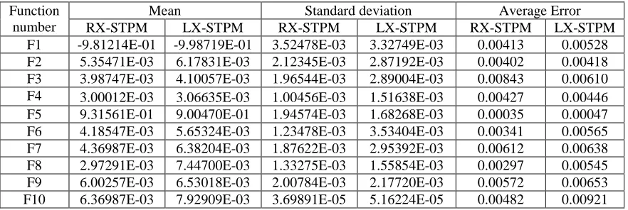
Table 3 depicts the findings of average error,
mean and standard deviation of the best objective function values. These performance measures are aimed at comparing the quality of the solutions found. RX-STPM achieved lower mean objective function values while the corresponding standard deviations for all the problems except function no 1, and 5. Furthermore, it is apparent that RX-STPM performs far better than LX-RX-STPM on average error for all the problems except function no. 3. Table 3 results indicate the supremacy of RX-STPM over LX-STPM. It proved RX-STPM to be a far more accurate algorithm.
7. CONCLUSIONS
This paper purports a real coded crossover operator based on Rayleigh distribution called Rayleigh Crossover (RX). An existing real coded crossover called Laplace Crossover (LX) is compared with the performance of RX. To justify the comparison, both of the crossover operators made use of the same mutator we defined earlier called Scale Truncated Pareto Mutator, STPM. Hence, two (2) generational real coded genetic algorithms (RCGAs) are designed called RX-STPM and LX-STPM. We set up the optimal parameters and used Ten (10) diverse and unbiased chosen set of standard benchmark functions to examine the performance analysis of RX-STPM and LX-STPM.
the criteria. In summary, the experimental results demonstrated that RX-STPM is a more efficient, reliable and accurate algorithm as compared to LX-STPM. The present study compared the performance between RX and LX. Future studies can look into many aspects to improve the performance of RX.
APPENDIX A: TEN (10) BENCHMARKING FUNCTIONS
Function no. 1 to 5 are nonscalable and function no. 6 to 10 are scalable. All the ten (10) benchmarking functions which are used to perform the current study have varying properties in terms of complexity and modality. The number of variables for all the scalable benchmarking functions is fixed at 30. In a scalable function, the number of decision variable can be heightened or reduced as required. A multimodal function only has one global optimum but has many local optima. When the dimensionality of a problem escalates, the search space will increase exponentially to the difficulty of a problem. As such, the potential for separation is a gauge of the difficulty of benchmark functions. The properties involved in said processes to determine the optimization level is elaborated in [27].
A) The Formulas And Features Of Five (5) Nonscalable Functions Are Given Below:
1. Easom 2D (Unimodal)
The global minimum has a small area relative to the search space.
Min f (x) = -cos(x1)cos(x2)exp(-(x1-π)2-( x2-π)2)
subject to -10 ≤ x1, x2 ≤ 10. The global minimum
is located at x* = f (π, π) and f (x*) = -1
2. Becker and Lago (Unimodal)
Min f (x) = (|x1| - 5)2 + (|x2| - 5)2
subject to -10 ≤ x1, x2 ≤ 10. The function has four
minima located at x* = f (±5, ±5), all with f (x*) = 0
3. Bohachevsky 1 (Continuous, differentiable, separable, non-scalable, multimodal)
Min f (x) = x12 + 2x22 - 0.3cos(3πx1) -
0.4cos(4πx2) + 0.7
subject to -50 ≤ x1, x2 ≤ 50. The global minimum
is located at x* = f (0, 0) and f (x*) = 0
4. Eggcrate (Continuous, separable, non-scalable)
Min f (x) = x12 + x22 + 25(sin2x1 + sin2x2)
subject to -2π≤ x1, x2 ≤ 2π. The global minimum
is located at x* = f (0, 0) and f (x*) = 0
5. Periodic (Separable)
Min f (x) = 1 + sin2x1 + sin2x2 - 0.1exp(-x12 - x22)
subject to -10 ≤ x1, x2 ≤ 10. The global minimum
is located at x* = f (0, 0) and f (x*) = 0.9
B) The Formulas And Features Of Five (5) Scalable Functions Are Given Below:
6. Sphere (Continuous, differentiable, separable, scalable, multimodal. This function is easily converge to the global optimum)
Min fx x
n
i=1
subject to -5.12 ≤ xi ≤ 5.12. The global minimum
is located at x* = f (0, 0, ..., 0) and f (x*) = 0
7. Rosenbrock (Continuous, differentiable, non-separable, scalable, unimodal)
Min fx 100x ! x! x 1
n-1
i=1
subject to -30 ≤ x1 ≤ 30. The global minimum is located at x* = f (1, 1, 1, ..., 1) and f (x*) = 0
8. Rastrigin (Non-linear multimodal. This function is fairly difficult due to the large search space and large number of local minima.)
Min fx 10n ! x 10cos 2πx
n
i=1
subject to -5.12 ≤ xi ≤ 5.12, i = 1, ..., n. The global minimum is located at x* = f (0, 0, ... , 0) and f (x*) = 0
Min fx |x| ! % x
" n
i=1
subject to -10 ≤ x1 ≤ 10. The global minimum is located at x* = f (0, 0, ... , 0) and f (x*) = 0
10. Griewank (Continuous, differentiable, non- separable, scalable, multimodal)
Min fx 1 !4000 x1 % cos 'x
√i)
" n
i=1
subject to -600 ≤ xi ≤ 600. The global minimum is
located at x* = f (0, 0, ..., 0) and f (x*) = 0
REFERENCES
[1] Liberti L, Kucherenko S. Comparison of deterministic and stochastic approaches to
global optimization. International
Transactions in Operational Research 2005; 12: 263-285
[2] Holland JH. Adaption in Natural and Artificial Systems: University of Michigan press. 1975 [3] Fogel LJ. Toward Inductive Inference
Automata. In Proceedings of the International
Federation of Information Processing
Congress. Munich 1962: 395-399
[4] Rechenberg I. Cybernetic solution path of an experimental problem 1965
[5] Darwin C, Beer G. The origin of species: Oxford University Press. 1951
[6] De Jong KA. Genetic Algorithms are NOT Function Optimizers. 1992: 5-17
[7] J. Antonisse. A new interpretation of schema notation that overturns the binary encoding constraint, in J.David Schaffer (Ed.) 1989, pp. 86-91
[8] Wright AH. Genetic Algorithms for Real Parameter Qptimization, in: G.J.E. Rawlins (Ed.). Foundations of Genetic algorithms I, 1990: 205-218
[9] Herrera F, Lozano M, Verdegay JL. Tackling real-coded genetic algorithms: Operators and tools for behavioural analysis. Artificial Intelligence Review 1998; 12: 265-319 [10] Ono I, Satoh H, Kobayashi S. A real-coded
genetic algorithm for function optimization using the unimodal normal distribution crossover. Transactions of the Japanese Society for Artificial Intelligence 1999; 14: 1146-1155
[11] Z. Michalewicz. Genetic algorithms + data structures = evolution programs: Springer. 1996
[12] Deep K, Thakur M. A new crossover operator for real coded genetic algorithms. Applied Mathematics and Computation 2007; 188: 895-911
[13] Goldberg DE. Genetic Algorithms in Search, Optimization and Machine Learning. New York: Addison-Wesley. 1989
[14] Eshelman LJ. Crossover operator biases: Exploiting the population distribution 1997: 354-361
[15] Syswerda G. Uniform crossover in genetic algorithms 1989
[16] Radcliffe NJ. Equivalence class analysis of genetic algorithms. Complex Systems 1991; 5: 183-205
[17] Schlierkamp-Voosen D. Predictive models for the breeder genetic algorithm. Evolutionary computation 1993; 1: 25-49
[18] Agrawal RB, Deb K, Agrawal RB. Simulated binary crossover for continuous search space 1994
[19] Eshelman LJ. chapter Real-coded Genetic
Algorithms and Interval-Schemata.
Foundations of genetic algorithms 1993; 2: 187-202
[20] Moraglio A, Poli R. Topological interpretation of crossover 2004: 1377-1388
[21] Tsutsui S, Yamamura M, Higuchi T. Multi-parent recombination with simplex crossover in real coded genetic algorithms 1999; 1: 657-664
[22] Mühlenbein H, Schlierkamp-Voosen D. Predictive models for the breeder genetic
algorithm i. continuous parameter
optimization. Evolutionary computation 1993; 1: 25-49
[23] Voigt H, Mühlenbein H, Cvetkovic D. Fuzzy
recombination for the breeder genetic
algorithm 1995
[24] Lim SM, Sulaiman MN, Md Sultan AB, Mustapha N, Ario Tijo B. Real coded genetic algorithm (RCGA): a new RCGA mutator called Scale Truncated Pareto Mutation.
Journal of Theoretical and Applied
Information Technology 2014; Volume 60, Issue 2
[26] Deep K, Katiyar V. A new real coded genetic algorithm operator: log logistic mutation 2012: 193-200
[27] Jamil M, Yang X. A literature survey of benchmark functions for global optimisation
problems. International Journal of
[image:7.612.89.526.205.256.2]Mathematical Modelling and Numerical Optimisation 2013; 4: 150-194
Table 1: Parameter Setting For RX-STPM And LX-STPM
GA name Nonscalable Scalable
Pc Pm Ts Pc Pm Ts
RX-STPM 0.70 0.01 2 0.60 0.03 2
[image:7.612.125.488.295.447.2]LX-STPM 0.65 0.02 3 0.70 0.003 5
Table 2: Computational Results Of AFE And SR For All Ten (10) Problems
Function number
Average Function Evaluation Success Rate
RX-STPM LX-STPM RX-STPM LX-STPM
F1 89 129 100 100
F2 156 183 100 100
F3 897 636 100 100
F4 220 249 100 100
F5 185 103 100 80
F6 27,143 29,036 100 100
F7 123,879 152,254 90 85
F8 104,145 111,848 100 100
F9 62,158 40,573 78 95
F10 57,159 60,392 100 100
Table 3: Computational Results Of Average Error, Mean Of Objective Function And Its Corresponding Standard Deviation For All Ten (10) Problems.
Function number
Mean Standard deviation Average Error
RX-STPM LX-STPM RX-STPM LX-STPM RX-STPM LX-STPM
F1 -9.81214E-01 -9.98719E-01 3.52478E-03 3.32749E-03 0.00413 0.00528
F2 5.35471E-03 6.17831E-03 2.12345E-03 2.87192E-03 0.00402 0.00418
F3 3.98747E-03 4.10057E-03 1.96544E-03 2.89004E-03 0.00843 0.00610
F4 3.00012E-03 3.06635E-03 1.00456E-03 1.51638E-03 0.00427 0.00446
F5 9.31561E-01 9.00470E-01 1.94574E-03 1.68268E-03 0.00035 0.00047
F6 4.18547E-03 5.65324E-03 1.23478E-03 3.53404E-03 0.00341 0.00565
F7 4.36987E-03 6.38204E-03 1.87622E-03 2.95392E-03 0.00612 0.00638
F8 2.97291E-03 7.44700E-03 1.33275E-03 1.55854E-03 0.00297 0.00545
F9 6.00257E-03 6.53018E-03 2.00784E-03 2.17720E-03 0.00572 0.00653
[image:7.612.87.528.507.655.2]