Swarm Engineering for Agent-Based Economics

Swarm Engineering for Agent-Based Economics

Sanza Kazadi

, Paul Kim

, John Lee

, Joshua Lee

Abstract— TheHamiltonian Method of Swarm De-sign is applied to the design of an agent based eco-nomic system. The method allows the design of a sys-tem from the global behaviors to the agent behaviors, with a guarantee that once certain derived agent-level conditions are satisfied, the system behavior becomes the desired behavior. Conditions which must be sat-isfied by consumer agents in order to bring forth the ”invisible hand of the market” [18] are derived and demonstrated in simulation. A discussion of how this method might be extended to other economic systems and non-economic systems is presented.

Keywords: swarm engineering, Hamiltonian method of swarm design, swarm economics

1

Introduction

Complex system design is a challenging field of science in which some to many independent interacting parts are combined so as to create a machine or system with a particular desired function or property set. A subset of the general field of complex systems is swarms, which are groups of bidirectionally communicating autonomous agents. Swarms are interesting for a number of reasons, the most important of which is the tendency of swarms to exhibitemergence, which allows them to undertake ac-tions that are not explicitly part of the control algorithm.

The most challenging thing in complex system design is ensuring that the different parts will interact with each other in a such a way as to generate a desired system behavior. This is particularly true for systems of au-tonomous agents. Since each agent is independent, the interactions can be very difficult to predict, a priori.

In the swarm literature, there is little in the way of gen-erally applicable principalled approach to swarm design. Some researchers [21, 17] have built preliminary systems for monitoring or understanding the emergent behaviors of agents. However, these studies do not yet generalize to a methodology that works for a large number of swarm systems. As a result, no particular method exists for gen-erating swarms of particular design.

In this paper, we examine what we call the

Hamilto-∗_{Jisan Research Institute Email: [email protected] To whom}

correspondences should be addressed.

†_{Jisan Research Institute Email: [email protected]}

‡_{Jisan Research Institute Email: [email protected]}

§_{Jisan Research Institute Email: [email protected]}

nian Method of Swarm Design (HMOSD)[6]. This method is a principalled approach to swarm design con-sisting of two main phases. In the first phase, the global goal(s) is(are) written in terms of properties that can be sensed and affected by the agents. The resulting equa-tion(s) can then be used to develop requirements for the behaviors of the agents that lead to the global goal.

Though swarm engineering has typically been applied to robotic design and computation design, we broaden the scope here by applying it to an economic system. So why economics? Economies are complex systems which en-compass micro and macro behaviors, individual interac-tion, equilibriums, and, in most cases, some sense of self-regulation [17]. Because of this overwhelming complexity, a quantitative form of economics has been difficult to ob-serve. However, with more powerful computational power and the development of efficient control algorithms it is now possible to approach economics from a more quanti-tative, rather than theoretical, perspective [4][5][11]. One such control method is swarm engineering. Just as a real economy is decentralized, automated swarms require no outside control [6]. An accurate simulation can be run solely by itself, basic economics laws and theories gov-erning the physics of interaction of agents. An advantage of this method is the lack of the ceteris paribus (Latin for “all other things unchanged”) aspect of traditional eco-nomics. Observations qualified by ceteris paribus require that all other variables in a causal relationship are ruled out in order to simplify studies. A swarm controlled simu-lation, on the other hand, allows all factors to be included in the relationship between antecedent and consequent [6][7]. Another salient advantage is an observer’s ability to control the basic structure of interaction. Before a run, the simulation allows one to tinker with basic parameters of the system, such as sizes of budgets, rate of utility in-crease, and the magnitude of competition. By allowing such control, a user can predict results of economies in several types of real-life situations, which is key in under-standing the scope of economic systems and the realistic range of our control.

inter-actions between agents define what the economy will do [1, 4, 8, 10, 11, 12, 15, 16, 19]. However, though these studies extracted global behaviors from their systems, they did not develop or apply a method of generating the global behavior, and then designing the system around that behavior. This study, which might be termed a study inswarm economics, is meant to examine the de-sign phase of an economic system using the swarm engi-neering methodology.

The remainder of the paper is organized as follows. Section 2 examines the theoretical application of the HMOSD to a simple economic model. This section fo-cuses on the properties of the agents that will give the economy a particular behavior. Section 3 presents the performance of the model under different expected agent behaviors. Section 4 offers some discussion and conclud-ing remarks.

2

Swarm Engineering Applied to

Eco-nomic Systems

In this section, we will theoretically explore the applica-tion of the principles of swarm engineering to economic systems. In swarm engineering, we are primarily inter-ested in generating group behaviors by utilizing careful examination of the desired global behavior and using this analysis to guide the design of agent-level behaviors ca-pable of producing the desired global behavior [6]. While this method still requires considerable input from the en-gineer, we have been able to use it to solve previously un-solved problems in deployment of swarms. In the present study, this means that we are interested in examining one or more global economic measurables and putting together a method of directly manipulating these by de-signing specific agent behaviors.

In economic systems, there are many global measurables. Each one is tied to local variables in a complicated and non-linear way. This makes the prediction of the global effect of a specific local behavior very difficult. As a re-sult, it is often times simpler to utilize agent-based sys-tems to get an idea of the effect of specific behaviors. The difficulty with utilizing agent-based systems in this way derives from the difficulty in creating a new system with specific desired qualities; the nonlinearity of com-plex systems makes this a very difficult thing to do. As a result, we utilize the swarm engineering methodology, which draws its initial motivation from the desired global outcome.

As our global property, we choose a truly dispersed prop-erty – that of the average cost of a commodity across ven-dors for sales of specific commodities. This property is in-teresting because it measures how much a consumer pays for goods and services that are worth a specific amount. If all vendors tend to end up with similar prices, this in-dicates that either the system is designed to enforce a

specific price, or that there is some kind of communica-tion between vendors that allows them to collude. We shall see that there are specific system designs that allow the former to occur without collusion or any communica-tion between vendors.

We examine the design of consumer behavior as a method of controlling the average price. Vendors are modelled as profit maximizers who will increase their prices when all else is kept constant. The reaction of the consumers must be made in such a way that slow creeping price increase does not occur. We shall see that specific agent behaviors, designed properly, can limit the average prices to prices that very closely match the cost of vending the product.

2.1 Vendors and consumers

We begin by modelling the main factors that affect the vendors in their decision to alter prices of commodities that they are selling. We begin with the assumption that all vendors will choose a price for a commodity that equals or exceeds his or her costs incurred during the sale of the commodity. The question then is what factors affect the change in the price?

We begin by assuming that the price function used by a vendor is a complicated function of several different values. That is, let the price be represented as

pv,c=f(m1, m2, . . . , mn). (1)

Then, each of these valuesmi represents a factor in de-termining the price of the commodity.

There are many factors one might include in a decision about the cost of a commodity or in a decision about whether or not to increase the cost of a commodity. Among these factors are the demand for the commod-ity (D), the vendor’s account balance (b), the total cost of the commodity to the vendor including the cost to put it on the shelf (space, cost outlays, and personnel) (cc), any memorized or recorded data of the pastlcycles ({mj}lj=1), and the current income of the vendor (i). We

assume, for the moment, that these are the main effectors of the cost of the commodity.

As we stated above, our goal is to examine the dynamics of the average price of specific commodities. This is the average price over all vendors of the commodity. I.e.,

Pa,c= 1 Nv

Nv

v=1

pv,c (2)

where Pa,c is the average price for commodity c, Nv is the number of vendors, andpv,c is vendor v’s price for the commodityc.

time. However, theoretical prices should actually de-crease or remain stable over time as the cost of production decreases. Moreover, the market is assumed to produce corrections to initially poorly priced items (i.e. items whose prices are much higher than the cost to produce it). We are interested in discovering what the minimal conditions are for consumers which will result in com-modity prices that decrease or stabilize over time. This can be written mathematically as

dPa,c dt = 1 Nv Nv i=1 dpv,c

dt ≤0. (3)

If a single vendor’s prices start decreasing, then under competitive conditions, all vendors’ prices should start decreasing. This being the case, we don’t expect one vendor’s price to increase while any of the other vendors’ prices decrease. As a result, we can replace the require-ment of (3) with

dpv,c

dt ≤0. (4)

If we begin by assuming that the vendors have a system-atic method to their pricing choices, then we may write the prices faced by consumers as (1). Utilizing the various measurements indicated above, this means that

dpv,c dt = ∂f ∂D dD dt + ∂f ∂b db dt+ ∂f ∂cc dcc dt + l j=1 ∂f ∂mj dmj dt + ∂f ∂i di dt. (5)

The term in (5) _∂cc∂f dcc_dt would seem to have little to do with the consumers, and so cannot be directly affected by a behavioral change among consumers. We therefore ignore it as a potential design point. On the other hand, it is interesting to note that db

dt is the rate at which the bank account changes. Thus, we identify this with the profit. If profit isP rthen,

P r(t) = db

dt =D(t) (f(t)−cc(t)). (6) where D(t) represents the number sold per time pe-riod. Moreover, this profit/loss may be memorized by the agent, affecting behavior. For each vending agent, the behavior can be different, but in general

mk(t) =P r(t−ktp) =D(t−ktp) (f(t−ktp)−cc(t−ktp)) (7) where tp represents a time period and k represents the specific memory element being stored. k typically runs from 1 throughNm, the number of memory elements used in the function.

Since we are examining conditions that make dpv,c_dt a non-increasing function of time in the absence of inflation and supply variations, we want

0≥ ∂f ∂D dD dt + ∂f ∂b db dt+ ∂f ∂cc dcc dt + ∂f ∂mp/l dmp/l dt + ∂f ∂i di dt. (8)

As a result, we have that ∂f

∂D dD

dt ≤ −

∂f ∂b db dt+ ∂f ∂cc dcc dt + ∂f ∂mp/l dmp/l dt + ∂f ∂i di dt (9) Inserting the results of (6) and (7) reveals that the actual form of this equation becomes

∂f ∂D

dD dt ≤ −

∂f

∂b(D(t) (f(t)−cc(t))) + ∂f ∂cc dcc dt + ∂f ∂i di dt − k ∂f ∂mp/lD

(t−ktp) (f(t−ktp)−cc(t−ktp))

(10) In the case that the vendor simply reacts to current con-ditions, the relation takes the form

∂f ∂D

dD dt ≤ −

∂f

∂b(D(t) (f(t)−cc(t))) + ∂f ∂cc dcc dt + ∂f ∂i di dt . (11) Now, we examine (10) to determine the form off.

1. If the cost to the vendor increases, it is reasonable to expect the vendor to either increase or hold steady its prices. That is

dcc dt >0⇒

∂f ∂cc >

0. (12)

2. If the income increases, one can infer that the de-mand at a particular price has increased. There-fore, by increasing the price, the profit will increase. Thus, we expect that

∂f

∂i >0. (13)

3. If profit increases, one can infer that the demand at a particular price has increased. Therefore, by increasing the price, the profit will increase. Thus, we expect that

∂f ∂b >0.

4. If the demand increases, typically the price increases. Therefore we expect that

∂f ∂D>0

These results together give us that

dD dt ≤ −

1 ∂f ∂D

∂f

∂b(D(t) (f(t)−cc(t))) + ∂f ∂cc dcc dt + ∂f ∂i di dt − k ∂f ∂mp/lD

(t−ktp) (f(t−ktp)−cc(t−ktp))

or in the case that the agents are purely reactive

dD dt ≤ −

1 ∂f ∂D

∂f

∂b(D(t) (f(t)−cc(t))) + ∂f ∂cc

dcc dt +

∂f ∂i

di dt

.

(15)

We have just proved the following theorem.

Theorem 2.1 If the condition in equations (14) or (15) continually holds, then the price will be bounded above.

These last two equations give the limits of the behav-ior of the consumer agents in a system composed of the vendor and consumer agents only. It indicates that the consumer agents must respond with a decrease in the demand for a commodity which is greater in magnitude than the magnitude of the right hand side of equations (14) and (15). This is a severe design requirement on the consumer agents. However, as we will see in the next section, systems containing consumer agents which fol-low these restrictions do tend to have the desired global characteristics, while those that do not tend to have sig-nificantly higher to run-away prices.

2.2 Design of consumer agents

Our primary concern is that the consumer agents prov-ably behave in such a way that the global average price remains bounded above. We have already seen in section 2.1 that if the conditions in equations (14) and (15) are obeyed, the goal will be achieved. That completes the top-down portion of the design problem. We now have an engineering requirement with which to work. We can now begin the bottom-up phase.

In this new phase, we must generate agents that satisfy this requirement. The general solution to the general equation given in (15) if ∂f_∂i = dcc_dt = 0, _∂D∂f =α, and∂f_∂b = γ, the general solution is

D=e− t 0−

γ

α(f(t)−cc(t))dt_{. (16)}

As a result of this general solution, it is clearly the case that, in order to react correctly in the next time frame, our agents must have the following capabilities.

1. The agents must be able to measure the price of the commodity.

2. The agents must be able to measure the demand for the commodity. In our simulations, it is a good estimate to know one’s own probability of purchasing the commodity and multiplying by the population size.

3. The agents must be able to accurately estimate the cost to the vendor.

Thus, all agents must have this capability, and their be-havior must be one of this family of bebe-haviors. We can write this as an update rule. This becomes

Di+1=Di

1− γ

α(fi−cci)

. (17)

This equation underscores the idea that the demand will remain constant when the price is near the cost. However, as the vendors will constantly be trying to increase the price, and the consumers will be reacting to increases, the actual average price will be greater than the cost to vendors. It is worth noting, of course, that in the real world, this cost is replaced by a very poorly defined notion of the ”value” of an object. Since consumers have no idea, in general, how much a specific object actually costs in real terms, they must guess about it’s value. However, despite this ignorance-driven inflation, the prices, once equilibrated, must respond to the same type of force.

In the next section, we describe our simulation and the behaviors of the agents carrying out repeated cycles of interactions between consumers and vendors. We gener-ate a family of behaviors parametrized by a small number of parameters. Some values of the parameters generate behaviors that obey the requirements of (15) and some do not. We explore the effects of these parameters and demonstrate that they yield the expected global behav-iors.

3

Simulation Design

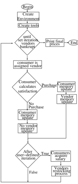
We examine our theoretical results using a computer sim-ulation that centers around the interactions between two types of agents: consumers and vendors. Our simulation functions by creating repeated interactions between the consumers and vendors as they learn and react to certain situations [19]. Vendors have commodities to sell, and are designed to maximize profit. Consumers purchase com-modities from vendors using money provided to them by jobs, and attempt to maximize consumption. The simu-lation proceeds by repeated “sessions” during which con-sumers visit vendors, evaluate what the vendors have to offer, and decide whether or not to buy. Vendors respond to changes in their products’ marketability by changing prices in an attempt to increase their profit.

the function of the system.

Begin

Create Environment

Create tools

set iteration bankruptvendors

. until

vendor assigned

Consumer

satisfaction calculates

Purchase Purchase

Consumer update memory

memory update

Consumer memory

update

Vendor consumer is

memory update No

No vendor

user−defined iteration

After _{True Consumers} acquire

salary

Vendors restocking

process Print final

prices End

False

Figure 3.1: This is a general flowchart of ABES

3.1 Vendors

As soon as ABES is executed, the products are assigned a random cost. Each vendor sells a single commodity, and so must assign and manage the price of the single commodity. Each vendor calculates its own minimum price. Initially, the price is set at twice the cost to the vendor. All the profits made from a completed exchange is directly added to the vendor’s bank account, the total amount of money that the vendor has. The vendor will re-stock its inventory when the number of products it holds reaches a user defined number if there is enough money in the bank to purchase more products. If the vendor fails to restock using the amount of money in the bank, then that vendor is considered bankrupt and is removed from the pool of vendors. As a result, the bankrupt vendor no longer participates in the interactions between vendors any consumer.

Each vendor’s goal is to maximize its profit by any means.

After a user-defined number of iterations, if the vendor has made more profit than it did in the previous period, the prices of the vendor’s product are incremented by a constant, user defined percentage of the product’s cost. This price update rule comes from the assumption that vendors will expect the same number (or nearly the same number) of products to sell the next period. A slight increase of price will increase the total profit. Conversely, if the vendor has made less profit, it reduces its prices by the same percentage. This behavior of decreasing the price derives from the assumption that the vendor will sell more the next period by slightly decreasing the price. This should increase the total profit.

3.2 Consumers

Behaviors of our consumers are similar to consumers in [16]. Each consumer interacts with its vendor in the same way: the consumer buys from the vendor if all of the con-ditions are met each time the consumer randomly chooses a vendor to buy the commodity from. We assume the commodity is something the consumer eventually must buy, like water. If the consumer waits long enough, it will be forced by necessity to purchase the commodity at any price. If the consumer has enough money, the item is in stock, the vendor is not bankrupt, and the consumer is “satisfied” with the product, the consumer will pur-chase the product. The consumer’s satisfaction with the vendor’s products is represented by a number from 0 to 100, and is affected by the length of time since the last purchase, the consumer’s memory of the prices, and the vendor’s profit margin. Along with the information in the consumer’s memory, the consumer calculates its sat-isfaction toward the product. A random number from 0 to 100 is generated, and if the calculated satisfaction is higher than the generated number, then the consumer will be considered “satisfied” enough to buy the product. Thus, the higher the satisfaction of the consumer is, the more likely the consumer is to purchase an item from the vendor. Each consumer’s cache of money is incremented by a user defined salary after some number of iterations, and decremented by the amount of each purchase.

constantly increasing their price and will result in a sta-blized price. However, as we will see in the next section, there are strict limits on even this behavior which yield control on global price levels.

In our simulation, we model the consumer satisfaction as

S=smax[1−( 1

et−[α(prof it)+(price−γ(pricemem))])] (18)

HereSis the satisfaction,αis a constant that controls the consumer’s aversion to profit margin, andγis a constant that affects competition among vendors. Both of these variables can be initially assigned different values. Profit is the amount of money the vendors make after an ex-change is complete. Price is the current price of the com-modity and pricemem is the running average of the prices paid by the individual consumer during the last several interactions for the same commodity. The higher the ex-ponent value, higher the satisfaction. Clearly, changing the value ofαwill alter the consumer’s sensitivity toward the profit. Likewise,γ affects the consumer’s sensitivity to prices much higher than those recently paid. This in-directly affects competition between vendors.

4

Simulation data

In section 2, we examined the theoretical basis for the design of consumer agents which, we expect, are capa-ble of causing the ”invisicapa-ble hand of the market” to ap-pear, limiting the prices of commodities. Section 3 de-scribed our simulation. This simulation consisted of two kinds of agents – consumers and vendors. The two types of agents interact with each other, and have conflicting goals. Moreover, the consumers have a limitation that theymust have the commodity that is being sold, even-tually. Such a commodity might be like water. The con-sumer agents have the limitation that the longer they go without the commodity in question, the more they’re willing to tolerate to get it. As a result, there is potential for price gouging, leading to runaway prices.

In this section, we examine the behavior of the system under the action of the consumer agents. The agents’ behaviors are controlled by the equation (18). In this equation, there are two main parameters, α and γ. By changing the values of these parameters, we can produce differing agents behaviors. Some of these behaviors sat-isfy equation (15) and some don’t. We shall see that the desired outcome is achieved when equation (15) is satis-fied.

4.1 The effects of γ

In equation (18), we have two parameters, γ and α. γ primarily controls the effect of a high price with respect to previous experienced prices. A high value ofγ indicates a high sensitivity to higher prices while a low γ value indicates little or no effect. The overall effect is akin to

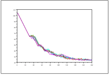
competition between individual vendors. With a high value ofγ, the prices tend to stabilize near those of the agent with the lowest prices, while lower values do not tend to reinforce this.

We can understand this in terms of equation (15). The demand does not change on the left hand side if the prices are all the same. However, the first term on the right hand side is large enough that the equation does not hold. As a result, the price does not reduce, but rather stays constant once all vendors have synchronized their prices. The situation is depicted in Figure 4.1.

0 100 200 300 400 500 600 700 50

60 70 80 90 100 110 120 130 140 150

0 10 20 30 40 50 60

54 55 56 57 58 59 60

Figure 4.1: With a high value ofγthe prices are limited to the lowest price of all consumers. However, if this lowest price is itself high, the prices will not rebound, as can be seen in these figures.

0 40 80 120 160 200 240 280 360

380 400 420 440 460 480

Figure 4.2: Even with a high value of_γ the prices can increase unboundedly if vendors continually increase their prices at similar rates.

4.2 Adding in α

It is clear that the competition between vendors is enough to hold most prices equal, but not strong enough to stabi-lize the cost of the commodities at prices that reflect their actual cost. This is interesting for a great many reasons, not the least of which is that this seems to contradict the ”invisible hand of the market” that underlies much of economic theory. Clearly, more than simple competition is required to restore this property.

Satisfying equation (15) requires that another, stronger term become active. In equation (18), the parameterα controls the sensitivity of the consumer to the profit mar-gin that the vendor is receiving. Very high values forα make the consumer intolerant of even small amounts of profit. On the other hand, small values for α make the consumer very tolerant of profits. We examine the effect of this.

The immediate effect is that the decrease in demand as a function of time becomes inextricably tied to the rate of increase of profit. If the profit increases, then the demand decreases. If αis high enough, the decrease exceeds any increase in overall profit associated with increasing the price. As a result, the condition in equation (15) is satis-fied, and the price is controlled. The situation is depicted in Figure 4.3.

0 20 40 60 80 100 120 140 160 180 20

30 40 50 60 70 80 90 100 110

Figure 4.3: Withγ high or low, a high value ofαis suf-ficient to control the prices of the commodity. This is ex-pected due to equation (15), and confirmed in this simula-tion.

Note that in subsection 4.1, we keptαlow, and the simu-lation had a global price increase over time. Only adding this very strong affector seems to hold prices low over time. The effect of this design element is so strong that it can take hold long after the price increase has begun, as illustrated in Figure 4.4.

0 40 80 120 160 200 240 280 320 360 400 30

50 70 90 110 130 150 170 190 210

Figure 4.4: If αis initially small, and γ high, the sys-tem exhibits slow price increase over time. However, ifα

is ”turned on” at some later time, the system recovers its low-price configuration.

4.3 Examining (15)

One of the main guiding principles of this study has been the need to satisfy equation (15) in generating the con-sumer behavior. The reason is that we showed in section 2 that if (15) is satisfied, then the behavior will lead to the desired global behavior. We now examine how closely our simulations adhere to this equation in generating the behaviors that limit commodity prices.

0 20 40 60 80 100 120 140 160 −1100

−700 −300 100 500 900 1300 1700

0 20 40 60 80 100 120 140 160 −5e+07

−4e+07 −3e+07 −2e+07 −1e+07 0e+00 1e+07 2e+07 3e+07 4e+07 5e+07

−1.0 −0.8 −0.6 −0.4 −0.2 0.0 0.2 0.4 0.6 0.8 1.0 0

1 2 3 4

−1.0 −0.8 −0.6 −0.4 −0.2 0.0 0.2 0.4 0.6 0.8 1.0 0

1 2 3 4 5

Figure 4.5: These graphs illustrate the values of equation (15) as the simulation is run (top two) and histogram the number of times it is obeyed and not obeyed (bottom two). We find that when the equation is obeyed most of the time (first and third), the prices are controlled. However, when the equation is obeyed considerably less than all the time (second and fourth), the prices are not controlled. This supports our theoretical derivation of this condition.

5

Discussion and conclusion

Designing swarms of agents is a very tricky business, ow-ing to the nonlinear interactions of the various agents. As with all complex systems, swarms of a particular design might have a particular global behavior, but swarms with a very slight difference in behavior may have completely

different global behaviors. As a result, predictive design has largely been avoided in the swarm literature.

In this paper, we’ve explored a method of swarm design in which a specific global swarm behavior is developed prior to the design of the agents. The desired behavior, it has been shown, can be made to order once a set of requirements for agent design is worked out which will mathematically guarantee that the swarm accomplishes the task [6]. Mathematical guarantee, which has eluded swarm researchers previously, is achieved by utilizing the global goal written in terms of the senses and actuators that the agents can be expected to have access to. Once the swarm condition has been met, the global goal may be achieved with agents meeting this condition.

It is interesting to note that this method of designing swarms is similar in form and function to the design of mechanical systems using the Lagrangian method. The power of this method lies in the ability of the engineer to create one or more properties whose numerical val-ues are unique to the state that the system is in. The engineer, then, needs only chart a path through the al-lowed phase space of the system to the final desired value, hopefully utilizing behaviors which individual agents can accomplish on their own, with or without guidance from a central controller. The method can be applied to sin-gle properties or to vectors of properties, provided that the desired vector is well-defined in the same way a single property might be. We believe that the method is so pow-erful, in fact, that we now coin a term for this method: The Hamiltonian Method of Swarm Design.

This study, which examines the design of an agent based economic system, has demonstrated that in such systems, the achievement of global goals is possible when specific agent traits are required of the agents. It is interest-ing that such systems can exhibit control that typically comes from ”the invisible hand of the market” or from a command economy [17]. In fact, we have unmasked the ”invisible hand of the market” in this study, revealing not only where it comes from but under what conditions it functions. It is interesting to ask, in light of the new method of controlling these swarms, what other economic indicators, trends, etc. can be commanded by the agents within the system.

prices. More research on this is clearly indicated.

In the future, we intend to apply this method to swarms of greater complexity than this one. We expect that this method of not only swarm design, but complex sys-tem design, may be applied to a large number of dif-ferent systems including, but not limited to, systems of autonomous mechanical agents, computing systems, eco-nomic systems, and social systems. While some of this research is currently under way, we expect that the ex-ploration of all fields to which this methodology might be applied will reveal an extraordinarily vast scope. More-over, we expect that an extension to this work will be able to solve the problem originally posed ten years ago which led us to these results: ”Is it possible that the global specification of a problem is enough to yield the basic requirements of the solution including all actuators, sensors, processing, and other capabilities of agents in the solution?” We believe the answer is yes.

References

[1] M. Chang, J. Harrington, Jr. Agent-Based

Mod-els of Organizations. Handbook of

Computa-tional Economics II: Agent-Based Conputa-tional Economics.March 24, 2005.

[2] S. Das.On Agent-Based Modeling of Complex

Sys-tems: Learning and Bounded Rationality.

Depart-ment of Computer Science and Engineering. La Jolla, CA, 92093-0404.

[3] M. Fisher, C. Ghidini.The ABC of Rational Agent

Modeling. Proceedings of the International

Joint Conference on Autonomous Agents and Multiagent Systems: Part 2, 849 - 856, Bologna, Italy, 2002.

[4] C. Hommes. Heterogeneous Agent Models in

Eco-nomics and Finance. Department of

Quantita-tive Economics, University of Amsterdam, March 2005.

[5] K.Judd, F. Kubler, K. Schmudders.Computational Methods for Dynamic Equilibria with Heterogeneous

Agents. World Congress, Cambridge University

Press, pp. 243 - 290, 2003.

[6] S. Kazadi.On the Development of a Swarm

Engi-neering Methodology. Proceedings of IEEE

Con-ference on Systems, Man, and Cybernetics,

Waikoloa, Hawaii, USA, pp. 1423 - 1428, October 2005.

[7] S. Kazadi.The Genesis of Swarm Engineering. Pro-ceedings of the SCI2003 Conference,

Spe-cial Session on Swarm Engineering, Orlando,

Florida, USA, 2003.

[8] G. Klein, A Fallah-Seghrouchni, P. Taillibert. An

Agent-Based Programming Method. Proceedings

of the International Joint Conference on Au-tonomous Agents and Multiagent Systems: Part 1, 4 - 7, Bologna, Italy, 2002.

[9] H. Knublauch. Extreme Programming of

Multi-Agent Systems. Proceedings of the

Interna-tional Joint Conference on Autonomous

Agents and Multiagent Systems: Part 2, 704 -711, Bologna, Italy, 2002.

[10] B. LeBaron. Agent Based Computational Finance.

Brandeis University, April 21st, 2005.

[11] J. Mackie-Mason, M. Weldman.Automated Markets

and Trading Agents. University of Michigan, Ann

Arbor, MI 48109, USA.

[12] R. Marks. Market Design Using Agent-Based Mod-els. The Universities of Sydney and New South Wales Sydney. May 17, 2005.

[13] P. Massonet, Y. Deville, C. Neve. From AOSE

Methodology to Agent Implementation.

Proceed-ings of the International Joint Conference on Autonomous Agents and Multiagent Sys-tems: Part 1, 27 - 34, Bologna, Italy, 2002.

[14] S. Mellouli, G. Mineau, D. Pascot. The Integrated Modeling of Multi-Agent Systems and Their

En-vironment. Proceedings of the International

Joint Conference on Autonomous Agents and Multiagent Systems.Bologna, Italy, 2002.

[15] P. Reitsma, P. Stone, J. Csirik, M. Littman.

Randomized Strategic Demand Reduction - Getting

More by Asking Less. Proceedings of the

In-ternational Joint Conference on Autonomous

Agents and Multiagent Systems: Part 1, 162

-163, Bologna, Italy, 2002.

[16] L. Said, T. Bouron, A. Drogoul.Agent-Based

Inter-action Analysis of Consumer Behavior.

Proceed-ings of the First International Joint Confer-ence on Autonomous Agents and Multiagent Systems: Part 1, 184 - 190, Bologna, Italy, 2002.

[17] Spears, William M. and Diana F. Gordon (1999).

Using Artificial Physics to Control Agents.IEEE

In-ternational Conference on Information, Intel-ligence, and Systems, November, 1999.

[18] J. Stiglitz, 1993,Economics, W. W. Norton & Com-pany, Inc, New York City, NY, 214 - 218 p.

[20] K. Tumer, A. Ayogino, D. Wolpert. Learning Se-quence of Actions in Collectives of Autonomous

Agents.Proceedings of the International Joint

Conference on Autonomous Agents and Mul-tiagent Systems: Part 1, 378 - 385, Bologna, Italy, 2002.

[21] Winfield, A., Sa, J., Gago, M.C., Dixon, C., Fisher,

M.On Formal Specification of Emergent Behaviours

in Swarm Robotics Systems. Int. J. Advanced

Robotic Systems, 2(4),363-370, 2005.

[22] G. Zhong, K. Takahashi, S. Amamiya. KODAMA

Project: From Design to Implementation of a

Distributed Multi-Agent System. Proceedings of

the International Joint Conference on Au-tonomous Agents and Multiagent Systems.