Original citation:
Pinski, F. J., Simpson, G., Stuart, Andrew M. and Weber, H.. (2015) Algorithms for
Kullback--Leibler approximation of probability measures in infinite dimensions. SIAM Journal on
Scientific Computing, 37 (6). A2733-A2757.
Permanent WRAP URL:
http://wrap.warwick.ac.uk/86356
Copyright and reuse:
The Warwick Research Archive Portal (WRAP) makes this work of researchers of the
University of Warwick available open access under the following conditions. Copyright ©
and all moral rights to the version of the paper presented here belong to the individual
author(s) and/or other copyright owners. To the extent reasonable and practicable the
material made available in WRAP has been checked for eligibility before being made
available.
Copies of full items can be used for personal research or study, educational, or not-for-profit
purposes without prior permission or charge. Provided that the authors, title and full
bibliographic details are credited, a hyperlink and/or URL is given for the original metadata
page and the content is not changed in any way.
Publisher’s statement:
First Published by SIAM Journal on Scientific Computing, 37 (6). A2733-A2757.
published by the Society for Industrial and Applied Mathematics (SIAM). Copyright © by
SIAM. Unauthorized reproduction of this article is prohibited.
A note on versions:
The version presented in WRAP is the published version or, version of record, and may be
cited as it appears here.
ALGORITHMS FOR KULLBACK–LEIBLER APPROXIMATION OF
PROBABILITY MEASURES IN INFINITE DIMENSIONS∗
F. J. PINSKI†, G. SIMPSON‡, A. M. STUART§, AND H. WEBER§
Abstract. In this paper we study algorithms to find a Gaussian approximation to a target measure defined on a Hilbert space of functions; the target measure itself is defined via its density with respect to a reference Gaussian measure. We employ the Kullback–Leibler divergence as a distance and find the best Gaussian approximation by minimizing this distance. It then follows that the approximate Gaussian must be equivalent to the Gaussian reference measure, defining a natural function space setting for the underlying calculus of variations problem. We introduce a computational algorithm which is well-adapted to the required minimization, seeking to find the mean as a function, and parameterizing the covariance in two different ways: through low rank
perturbations of the reference covariance and through Schr¨odinger potential perturbations of the
inverse reference covariance. Two applications are shown: to a nonlinear inverse problem in elliptic PDEs and to a conditioned diffusion process. These Gaussian approximations also serve to provide a preconditioned proposal distribution for improved preconditioned Crank–Nicolson Monte Carlo– Markov chain sampling of the target distribution. This approach is not only well-adapted to the high dimensional setting, but also behaves well with respect to small observational noise (resp., small temperatures) in the inverse problem (resp., conditioned diffusion).
Key words. MCMC, inverse problems, Gaussian distributions, Kullback–Leibler divergence, relative entropy
AMS subject classifications.60G15, 34A55, 62G05, 65C05
DOI.10.1137/14098171X
1. Introduction. Probability measures on infinite dimensional spaces arise in
a variety of applications, including the Bayesian approach to inverse problems [34] and conditioned diffusion processes [19]. Obtaining quantitative information from such problems is computationally intensive, requiring approximation of the infinite dimensional space on which the measures live. We present a computational approach applicable to this context: we demonstrate a methodology for computing the best approximation to the measure, from within a subclass of Gaussians. In addition we show how this best Gaussian approximation may be used to speed up Monte Carlo–Markov chain (MCMC) sampling. The measure of “best” is taken to be the Kullback–Leibler (KL) divergence, or relative entropy, a methodology widely adopted in machine learning applications [5]. In a recent paper [28], KL-approximation by Gaussians was studied using the calculus of variations. The theory from that paper provides the mathematical underpinnings for the algorithms presented here.
1.1. Abstract framework. Assume we are given a measureμon the separable
Hilbert space (H,·,·,·) equipped with the Borelσ-algebra, specified by its density with respect to a reference measure μ0. We wish to find the closest elementν toμ,
∗Submitted to the journal’s Methods and Algorithms for Scientific Computing section August 11,
2014; accepted for publication (in revised form) April 9, 2015; published electronically November 17, 2015.
http://www.siam.org/journals/sisc/37-6/98171.html
†Department of Physics, University of Cincinnati, Cincinnati, OH 45221 ([email protected]).
‡Department of Mathematics, Drexel University, Philadelphia, PA 19104 ([email protected].
edu). This author’s work was supported in part by DOE Award DE-SC0002085 and NSF PIRE Grant OISE-0967140.
§Mathematics Institute, University of Warwick, Coventry CV4 7AL, United Kingdom (a.m.
[email protected], [email protected]). The first author’s work was supported by EPSRC, ERC, and ONR. The second author’s work was supported by an EPSRC First Grant.
A2733
with respect to KL divergence, from a subsetAof the Gaussian probability measures onH. We assume the reference measure μ0 is itself a Gaussianμ0 =N(m0, C0) on
H. The measureμis thus defined by
(1.1) dμ
dμ0(u) = 1
Zμexp
−Φμ(u),
where we assume that Φμ : X → Ris continuous on some Banach space X of full
measure with respect to μ0, and that exp(−Φμ(x)) is integrable with respect to μ0. Furthermore,Zμ=Eμ0exp−Φ
μ(u)
ensuring thatμis indeed aprobabilitymeasure. We seek an approximation ν = N(m, C) of μ which minimizes DKL(νμ), the KL
divergence between ν and μ in A. Under these assumptions it is necessarily the
case that ν is equivalent1 to μ0 (we writeν ∼ μ0) since otherwise DKL(νμ) =∞. This imposes restrictions on the pair (m, C), and we build these restrictions into our algorithms. Broadly speaking, we will seek to minimize over all sufficiently regular functionsm, whilst we will parameterizeC either through operators of finite rank, or through a function appearing as a potential in an inverse covariance representation.
Once we have found the best Gaussian approximation we will use this to improve upon known MCMC methods. Here, we adopt the perspective of considering only MCMC methods that are well-defined in the infinite dimensional setting, so that they are robust to finite dimensional approximation [11]. The best Gaussian approximation is used to make Gaussian proposals within MCMC which are simple to implement, yet which contain sufficient information about Φμ to yield significant reduction in the autocovariance of the resulting Markov chain, when compared with the methods developed in [11].
1.2. Relation to previous work. In addition to the machine learning
appli-cations mentioned above [5], approximation with respect to KL divergence has been used in a variety of applications in the physical sciences, including climate science [15], coarse graining for molecular dynamics [22, 32], and data assimilation [3]. Our ap-proach is formulated so as to address infinite dimensional problems.
Improving the efficiency of MCMC algorithms is a topic attracting a great deal of current interest, as many important PDE based inverse problems result in target distributions μ for which Φμ is computationally expensive to evaluate. One family of approaches is to adaptively update the proposal distribution during MCMC, [1, 2, 17, 31]. We will show that our best Gaussian approximation can also be used to speed up MCMC and, although we do not interweave the Gaussian optimization with MCMC in this paper, this could be done, resulting in algorithms similar to those in [1, 2, 17, 31]. Indeed, in [1, 2] the authors use KL divergence (relative entropy) in the form DKL(μ||ν) to adapt their proposals, working in the finite dimensional setting. In our work, we formulate our strategy in the infinite dimensional context, and seek to minimize DKL(ν||μ) instead of DKL(μ||ν). Either choice of divergence measure has its own advantages, discussed below.
In [24], the authors develop a stochastic Newton MCMC algorithm, which resem-bles our improved preconditioned Crank–Nicolson MCMC (pCN-MCMC) Algorithm 5.2 in that it uses Gaussian approximations that are adapted to the problem within the proposal distributions. However, while we seek to find minimizers of KL in an offline computation, the work in [24] makes a quadratic approximation of Φμ at each step along the MCMC sequence; in this sense it has similarities with the Riemannian manifold MCMC methods of [16].
1Two measures are equivalent if they are mutually absolutely continuous.
As will become apparent, a serious question is how to characterize, numerically, the covariance operator of the Gaussian measureν. Recognizing that the covariance operator is compact, with decaying spectrum, it may be well-approximated by a low rank matrix. Low rank approximations are used in [24, 33], and in the earlier work [14]. In [14] the authors discuss how, even in the case whereμis itself Gaussian, there are significant computational challenges motivating the low rank methodology.
Other active areas in MCMC methods for high dimensional problems include the use of polynomial chaos expansions for proposals [25], and local interpolation of Φμto reduce computational costs [10]. For methods which go beyond MCMC, we mention the paper [13] in which the authors present an algorithm for solving the optimal transport PDE relatingμ0to μ.
1.3. Outline. In section 2, we examine these algorithms in the context of a
scalar problem, motivating many of our ideas. The general methodology is intro-duced in section 3, where we describe the approximation ofμ defined via (1.1) by a Gaussian, summarizing the calculus of variations framework which underpins our al-gorithms. We describe the problem of Gaussian approximations in general, and then consider two specific parameterizations of the covariance which are useful in practice, the first via finite rank perturbation of the covariance of the reference measure μ0, and the second via a Schr¨odinger potential shift from the inverse covariance of μ0. Section 4 describes the structure of the Euler–Lagrange equations for minimization, and recalls the Robbins–Monro algorithm for locating the zeros of functions defined via an expectation. In section 5 we describe how the Gaussian approximation found via KL minimization can be used as the basis for new MCMC methods, well-defined on function space and hence robust to discretization, but also taking into account the change of measure via the best Gaussian approximation. Section 6 contains il-lustrative numerical results, for a Bayesian inverse problem arising in a model of groundwater flow, and in a conditioned diffusion process, prototypical of problems in molecular dynamics. We conclude in section 7.
2. Scalar example. The main challenges and ideas of this work can be
exempli-fied in a scalar problem, which we examine here as motivation. Consider the measure μεdefined via its density with respect to the Lebesgue measure:
(2.1) με(dx) = 1
Zεexp
−ε−1V(x)dx, V :R→R.
ε > 0 is a small parameter. Furthermore, let the potential V be such that με is
non-Gaussian. As a concrete example, take
(2.2) V(x) =x4+12x2.
We now explain our ideas in the context of this simple example, referring to algorithms which are detailed later; additional details are given in Appendix A.
In order to link to the infinite dimensional setting, where Lebesgue measure is not defined and Gaussian measure is used as the reference measure, we writeμε via its density with respect to a unit Gaussianμ0=N(0,1):
dμε
dμ0 =
√
2π
Zε exp
−ε−1V(x) +12x2.
We find the best fit ν = N(m, σ2), optimizing DKL(νμ) over m ∈ R and σ > 0,
noting thatν may be written as
dν
dμ0 =
√
2π
√
2πσ2exp
− 1
2σ2(x−m)2+12x2
.
The change of measure is then
(2.3) dμ
ε
dν =
√
2πσ2
Zε exp
−ε−1V(x) +21
σ2(x−m)
2.
For potential (2.2),DKL, defined in full generality in (3.2), can be integrated analyt-ically, yielding
(2.4) DKL(ν||με) =12ε−12m4+m2+ 12m2σ2+σ2+ 6σ4−21+logZε−log√2πσ2.
In subsection 2.1 we illustrate an algorithm to find the best Gaussian approximation numerically while subsection 2.2 demonstrates how this minimizer may be used to improve MCMC methods. See [27] for a theoretical analysis of the improved MCMC method for this problem. That analysis sheds light on the application of our method-ology more generally.
2.1. Estimation of the minimizer. The Euler–Lagrange equations for (2.4)
can then be solved to obtain a minimizer (m, σ) which satisfiesm= 0 and
(2.5) σ2=241 √1 + 48ε−1=ε−12ε2+ O(ε3).
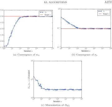
In more complex problems,DKL(νμ) is not analytically tractable and only defined via expectation. In this setting, we rely on the Robbins–Monro algorithm (Algorithm 4.1) to compute a solution of the Euler–Lagrange equations defining minimizers. Figure 1 depicts the convergence of the Robbins–Monro solution towards the desired root at ε= 0.01, (m, σ)≈(0,0.0950) for our illustrative scalar example. It also shows that DKL(νμ) is reduced.
2.2. Sampling of the target distribution. Having obtained values ofmand
σthat minimize DKL(νμ), we may useν to develop an improved MCMC sampling
algorithm for the target measure με. We compare the performance of the standard pCN method of Algorithm 5.1, which uses no information about the best Gaussian fitν, with the improved pCN Algorithm 5.2, based on knowledge ofν.The improved performance, gauged by acceptance rate and autocovariance, is shown in Figure 2.
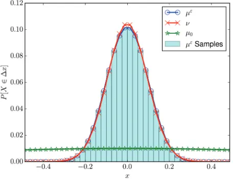
All of this is summarized by Figure 3, which shows the three distributions με, μ0, and KL optimizedν, together with a histogram generated by samples from the KL-optimized MCMC Algorithm 5.2. Clearly,ν better characterizesμεthanμ
0, and
this is reflected in the higher acceptance rate and reduced autocovariance. Though this is merely a scalar problem, these ideas are universal. In all of our examples, we have a non-Gaussian distribution we wish to sample from, an uninformed reference measure which gives poor sampling performance, and an optimized Gaussian which better captures the target measure and can be used to improve sampling.
3. Parameterized Gaussian approximations. We start in subsection 3.1 by
describing some general features of the KL distance. Then in subsection 3.2 we dis-cuss the case where ν is Gaussian. Subsections 3.3 and 3.4 describe two particular parameterizations of the Gaussian class that we have found useful in practice.
100 101 102 103 104 105 106 Iterationn
−0.10
−0.08
−0.06
−0.04
−0.02 0.00 0.02
mn
Exactm
(a) Convergence ofmn
100 101 102 103 104 105 106 Iterationn
10−2
10−1
100
σn
Exactσ
(b) Convergence ofσn
100 101 102 103 104 105 106 Iterationn
100
101
102
DKL
[
mn ,σn
]
+Constant
(c) Minimization ofDKL
Fig. 1.Convergence ofmn andσntowards the values found via deterministic root finding for
the scalar problem with potential (2.2)atε= 0.01. The iterates are generated using Algorithm4.1,
Robbins–Monro applied to KL minimization. Also plotted are values of KL divergence along the iteration sequence. The true optimal value is recovered, and KL divergence is reduced. To ensure convergence,mnis constrained to[−10,10]andσnis constrained to[10−6,103].
3.1. General setting. Letν be a measure defined by
(3.1) dν
dμ0(u) = 1
Zνexp
−Φν(u),
where we assume that Φν :X → Ris continuous on X. We aim to choose the best
approximation ν to μ given by (1.1) from within some class of measures; this class will place restrictions on the form of Φν.Our best approximation is found by choosing
the free parameters in ν to minimize the KL divergence between μ and ν. This is
defined as
(3.2) DKL(νμ) =
H log
dν dμ(u)
ν(du) =Eνlog
dν dμ(u)
.
Recall thatDKL(··) is not symmetric in its two arguments and our reason for choosing DKL(νμ) relates to the possibility of capturing multiple modes individually; mini-mizingDKL(μν) corresponds to moment matching in the case whereAis the set of all Gaussians [5, 28]. The moment matching form was also employed in the finite di-mensional adaptive MCMC method of [1, 2]. An advantage ofDKL(νμ) is that it can
[image:6.612.78.438.72.418.2]100 101 102 103 104 105 106 Iterationn
0.0 0.2 0.4 0.6 0.8 1.0
Acceptance
Rate
ν μ0
(a) Acceptance rate
100 101 102 103 104 105 106
Lagm
−0.2 0.0 0.2 0.4 0.6 0.8 1.0
Nor
maliz
ed
A
utoco
var
iance
ν μ0
(b) Autocovariance
Fig. 2. Acceptance rates and autocovariances for sampling from (2.1) with potential (2.2) at ε= 0.01. The curves labeledν correspond to the samples generated using our improved MCMC, Algorithm 5.2,which uses the KL optimizedν for proposals. The curves labeledμ0 correspond to
the samples generated using Algorithm 5.1,which relies onμ0 for proposals. Algorithm5.2shows
an order of magnitude improvement over Algorithm5.1. For clarity, only a subset of the data is plotted in the figures.
Fig. 3. Distributions of με (target), μ0 (reference), andν (KL-optimized Gaussian) for the
scalar problem with potential (2.2) at ε = 0.01. Posterior samples have also been plotted, as a histogram. By inspection,ν better capturesμε, leading to improved performance. Bins have width
Δx= 0.025.
capture detailed information about individual modes ofμ, in contrast toDKL(μν). See [28] for an elementary example with multiple modes.
Providedμ0∼ν, we can write
(3.3) dμ
dν(u) = Zν
Zμ exp
−Δ(u),
where
(3.4) Δ(u) = Φμ(u)−Φν(u).
Integrating this identity with respect toν gives
(3.5) Zμ
Zν =
H
exp−Δ(u)ν(du) =Eνexp−Δ(u).
[image:7.612.143.371.325.500.2]Combining (3.2) with (3.3) and (3.5), we have
(3.6) DKL(νμ) =EνΔ(u) + log
Eνexp−Δ(u).
The computational task in this paper is to minimize (3.6) over the parameters that characterize our class of approximating measures A, which for us will be subsets of Gaussians. These parameters enter Φν and the normalization constant Zν. It is noteworthy, however, that the normalization constants Zμ andZν do not enter this expression for the distance and are, hence, not explicitly needed in our algorithms.
To this end, it is useful to find the Euler–Lagrange equations of (3.6). Imagine that ν is parameterized by θ and that we wish to differentiate J(θ) := DKL(νμ) with respect to θ. We rewriteJ(θ) as an integral with respect to μ, rather than ν, differentiate under the integral, and then convert back to integrals with respect toν. From (3.3), we obtain
(3.7) Zν
Zμ =E
μeΔ.
Hence, from (3.3),
(3.8) dν
dμ(u) = eΔ
EμeΔ.
Thus we obtain, from (3.2),
(3.9) J(θ) =Eμ
dν dμ(u) log
dν dμ(u)
=E
μeΔ(Δ−logEμeΔ)
EμeΔ
and
J(θ) =E
μeΔΔ
EμeΔ −logEμeΔ.
Therefore, withD denoting differentiation with respect toθ,
DJ(θ) = E
μeΔΔDΔ
EμeΔ −
EμeΔΔEμeΔDΔ
EμeΔ2 .
Using (3.8) we may rewrite this as integration with respect toν and we obtain
(3.10) DJ(θ) =Eν(ΔDΔ)−(EνΔ)(EνDΔ).
Thus, this derivative is zero if and only if Δ andDΔ are uncorrelated underν.
3.2. Gaussian approximations. Recall that the reference measure μ0 is the
GaussianN(m0, C0).We assume thatC0 is a strictly positive-definite trace class op-erator onH[7]. We let{ej, λj2}∞j=1 denote the eigenfunction/eigenvalue pairs forC0. Positive (resp., negative) fractional powers ofC0 are thus defined (resp., densely
de-fined) onHby the spectral theorem and we may defineH1:=D(C−12
0 ), the Cameron–
Martin space of measureμ0. We assume that m0 ∈ H1 so that μ0 is equivalent to N(0, C0), by the Cameron–Martin theorem [7]. We seek to approximateμ given in (1.1) by ν ∈ A, where A is a subset of the Gaussian measures on H. It is shown
in [28] that this implies that ν is equivalent to μ0 in the sense of measures and this in turn implies thatν=N(m, C), wherem∈E and
(3.11) Γ :=C−1−C0−1
satisfies
(3.12) C12
0ΓC 1 2
0 2HS(H)<∞;
hereHS(H) denotes the space of Hilbert–Schmidt operators onH.
For practical reasons, we do not attempt to recover Γ itself, but instead introduce low dimensional parameterizations. Two such parameterizations are introduced in this paper. In one, we introduce a finite rank operator, associated with a vectorφ∈Rn. In the other, we employ a multiplication operator characterized by a potential function b. In both cases, the mean mis an element ofH1. Thus, minimization will be over either (m, φ) or (m, b).
In this Gaussian case the expressions forDKLand its derivative, given by equa-tions (3.6) and (3.10), can be simplified. Defining
(3.13) Φν(u) =−u−m, m−m0C0+12u−m,Γ(u−m) −12m−m02C0,
we observe that, assumingν∼μ0,
dν
dμ0 ∝exp
−Φν(u). (3.14)
This may be substituted into the definition of Δ in (3.4), and used to calculateJ and DJ according to (3.9) and (3.10). However, we may derive alternate expressions as follows. Letρ0=N(0, C0), the centered version ofμ0, andν0=N(0, C) the centered version ofν.Then, using the Cameron–Martin formula,
(3.15) Zν =Eμ0exp(−Φ
ν) =Eρ0exp(−Φν0) =
Eν0exp(Φ
ν0)
−1 =Zν0,
where
(3.16) Φν0= 12u,Γu.
We also define a reduced Δ function which will play a role in our computations:
(3.17) Δ0(u)≡Φμ(u+m)−12u,Γu.
The consequence of these calculations is that, in the Gaussian case, (3.6) is
DKL(ν||μ) =EνΔ−logZν0+ logZμ
=Eν0[Δ
0] + 12m−m02C0+ logE
ν0exp(1
2u,Γu) + logZμ. (3.18)
Although the normalization constantZμ now enters the expression for the objective function, it is irrelevant in the minimization since it does not depend on the unknown parameters inν. To better see the connection between (3.6) and (3.18), note that
(3.19) Zμ
Zν0 = Zμ
Zν =
Eμ0exp(−Φ
μ)
Eμ0exp(−Φν) =E
νexp(−Δ).
Working with (3.18), the Euler–Lagrange equations to be solved are
DmJ(m, θ) =Eν0D
uΦμ(u+m) +C0−1(m−m0) = 0, (3.20a)
DθJ(m, θ) =Eν0(Δ
0DθΔ0)−(Eν0Δ0)(Eν0DθΔ0) = 0.
(3.20b)
Here,θis any of the parameters that define the covariance operatorCof the Gaussian ν. Equation (3.20a) is obtained by direct differentiation of (3.18), while (3.20b) is obtained in the same way as (3.10). These expressions are simpler for computations for two reasons. First, for the variation in the mean, we do not need the full covariance expression of (3.10). Second, Δ0 has fewer terms to compute.
3.3. Finite rank parameterization. LetP denote orthogonal projection onto
HK := span{e1, . . . , eK}, the span of the firstK eigenvectors of C0, and defineQ=
I−P.We then parameterize the covarianceC ofν in the form
(3.21) C−1=QC0Q−1+χ, χ=
i,j≤K
γijei⊗ej.
In words, C−1 is given by the inverse covariance C0−1 of μ0 on QH, and is given by χ on PH. Because χ is necessarily symmetric it is essentially parameterized by a vector φ of dimension n = 12K(K+ 1). We minimize J(m, φ) := DKL(νμ) over (m, φ) ∈ H1×Rn.This is a well-defined minimization problem as demonstrated in Example 3.7 of [28] in the sense that minimizing sequences have weakly convergent subsequences in the admissible set. Minimizers need not be unique, and we should not expect them to be, as multimodality is to be expected, in general, for measuresμ defined by (1.1). Problem-specific information may also suggest better directions for the finite rank operator, but we do not pursue this here.
3.4. Schr¨odinger parameterization. In this subsection we assume that H
comprises a Hilbert space of functions defined on a bounded open subset of Rd.
We then seek Γ given by (3.11) in the form of a multiplication operator so that (Γu)(x) =b(x)u(x).While minimization over the pair (m,Γ), withm∈ H1 and Γ in the space of linear operators satisfying (3.12), is well-posed [28], minimizing sequences
{mk,Γk}k≥1 with (Γku)(x) =bk(x)u(x) can behave very poorly with respect to the sequence {bk}k≥1. For this reason we regularize the minimization problem and seek to minimize
Jα(m, b) =J(m, b) +α2b2r,
whereJ(m, b) :=DKL(νμ) and·rdenotes the Sobolev spaceHrof functions onRd with rsquare integrable derivatives, with boundary conditions chosen appropriately for the problem at hand. The minimization of Jα(m, b) over (m, b) ∈ H ×Hr is well-defined; see section 3.3 of [28].
4. Robbins–Monro algorithm. In order to minimize DKL(νμ) we will use
the Robbins–Monro algorithm [4, 23, 26, 30]. In its most general form this algorithm calculates zeros of functions defined via an expectation. We apply it to the Euler– Lagrange equations to find critical points of a nonnegative objective function, defined
via an expectation. This leads to a form of gradient descent in which we seek to integrate the equations
˙
m=−DmDKL, θ˙=−DθDKL,
until they have reached a critical point. This requires two approximations. First, as (3.20) involve expectations, the right-hand sides of these differential equations are evaluated only approximately, by sampling. Second, a time discretization must be introduced. The key idea underlying the algorithm is that, provided the step length of the algorithm is sent to zero judiciously, the sampling error averages out and is diminished as the step length goes to zero. Minimization of KL by Robbins–Monro was also performed in [1, 2] forDKL(μ||ν), in the case of finite dimensional problems.
4.1. Background on Robbins–Monro. In this section we review some of the
structure in the Euler–Lagrange equations for the desired minimization ofDKL(νμ). We then describe the particular variant of the Robbins–Monro algorithm that we use in practice. Suppose we have a parameterized distribution, νθ, from which we can generate samples, and we seek a valueθfor which
(4.1) f(θ)≡Eνθ[Y] = 0, Y ∼ν
θ.
Then an estimate of the zero,θ, can be obtained via the recursion
(4.2) θn+1=θn−an
M
m=1 1
MYm(n), Ym(n)∼νθn, i.i.d.
(where i.i.d. is independently and identically distributed). Note that the two approx-imations alluded to above are included in this procedure: sampling and (Euler) time discretization. The methodology may be adapted to seek solutions to
(4.3) f(θ)≡Eν[F(Y;θ)] = 0, Y ∼ν,
where ν is a given, fixed, distribution independent of the parameter θ. (This setup arises, for example, in (3.20a), where ν0 is fixed and the parameter in question is m.) Letting Z =F(Y;θ), this induces a distributionηθ(dz) =ν(F−1(dz;θ)), where the preimage is with respect to the Y argument. Then f(θ) =Eηθ[Z] withZ ∼η
θ, and this now has the form of (4.1). As suggested in the extensive Robbins–Monro literature, we take the step sequence to satisfy
(4.4)
∞
n=1
an=∞,
∞
n=1
a2n <∞.
A suitable choice of{an}is thusan=a0n−γ,γ∈(1/2,1]. The smaller the value ofγ, the more “large” steps will be taken, helping the algorithm to explore the configuration space. On the other hand, once the sequence is near the root, the smallerγ is, the larger the Markov chain variance will be. In addition to the choice of the sequencean, (4.1) introduces an additional parameter,M, the number of samples to be generated per iteration. See [4, 8] and references therein for commentary on sample size.
The conditions needed to ensure convergence, and what kind of convergence, have been relaxed significantly through the years. In their original paper, Robbins and
Monro assumed that Y ∼μθ were almost surely uniformly bounded by a constant
independent of θ. If they also assumed that f(θ) was monotonic and f(θ) > 0, they could obtain convergence in L2. With somewhat weaker assumptions, but still requiring that the zero be simple, Blum developed convergence with probability one [6]. All of this was subsequently generalized to the arbitrary finite dimensional case; see [4, 23, 26].
As will be relevant to this work, there is the question of the applicability to the infinite dimensional case when we seek, for instance, a mean function in a separable Hilbert space. This has also been investigated; see [12, 35] along with references mentioned in the preface of [23]. In this work, we do not verify that our problems satisfy convergence criteria; this is a topic for future investigation.
A variation on the algorithm that is commonly applied is the enforcement of constraints which ensure {θn} remain in some bounded set; see [23] for an extensive discussion. We replace (4.2) by
(4.5) θn+1= ΠD
θn−an
M
m=1 1
MYm(n)
, Ym(n)∼νθn, i.i.d.,
where D is a bounded set, and ΠD(x) computes the point in D nearest to x. This is important in our work, as the parameters must induce covariance operators. They must be positive definite, symmetric, and trace class. Our method automatically produces symmetric trace-class operators, but the positivity has to be enforced by a projection.
The choice of the setD can be set either through a priori information as we do here, or determined adaptively. In [9, 35], each time the iterate attempts to leave the current constraint set D, it is returned to a point within D, and the constraint set is expanded. It can be shown that, almost surely, the constraint is expanded only a finite number of times.
4.2. Robbins–Monro applied to KL. We seek minimizers of DKL as
sta-tionary points of the associated Euler–Lagrange equations, (3.20). Before applying Robbins–Monro to this problem, we observe that we are free to precondition the Euler–Lagrange equations. In particular, we can apply bounded, positive, invertible operators so that the preconditioned gradient will lie in the same function space as the parameter; this makes the iteration scheme well-posed. For (3.20a), we have found premultiplying by C0 to be sufficient. For (3.20b), the operator will be problem spe-cific, depending on howθ parameterizes C, and also if there is a regularization. We denote the preconditioner for the second equation by Bθ. Thus, the preconditioned Euler–Lagrange equations are
0 =C0Eν0D
uΦμ(u+m) + (m−m0), (4.6a)
0 =Bθ[Eν0(Δ
0DθΔ0)−(Eν0Δ
0)(Eν0D
θΔ0)]. (4.6b)
We must also ensure that m and θ correspond to a well-defined Gaussian; C must
be a covariance operator. Consequently, the Robbins–Monro iteration scheme is the following.
Algorithm 4.1.
1. Setn= 0. Pickm0andθ0 in the admissible set, and choose a sequence{an} satisfying(4.4).
2. Updatemn andθn according to
mn+1= Πm
mn−an
C0
M
=1 1
M ·DuΦμ(u)
+mn−m0
, (4.7a)
θn+1= Πθ
θn−anBθ
M
=1 1
M ·Δ0(u)DθΔ0(u)
−
M
=1
1
M ·Δ0(u) M
=1
1
M ·DθΔ0(u)
. (4.7b)
3. n→n+ 1 and return to 2.
Typically, we have some a priori knowledge of the magnitude of the mean. For instance, m∈H1([0,1];R1) may correspond to a mean path, joining two fixed end-points, and we know it to be confined to some interval [m, m]. In this case we choose
(4.8) Πm(f)(t) = min{max{f(t), m}, m}, 0< t <1.
For Πθ, it is necessary to compute part of the spectrum of the operator thatθinduces, check that it is positive, and, if it is not, project the value to something satisfactory. In the case of the finite rank operators discussed in section 3.3, the matrix γ must be positive. One way of handing this, for symmetric real matrices, is to make the following choice:
(4.9) Πθ(A) =Xdiag{min{max{λ, λ}, λ}}XT,
where A =Xdiag{λ}XT is the spectral decomposition, and λand λ are constants chosen a priori. It can be shown that this projection gives the closest, with respect to the Frobenius norm, symmetric matrix with spectrum constrained to [λ, λ] [20].2
5. Improved MCMC sampling. The idea of the Metropolis–Hastings variant
of MCMC is to create an ergodic Markov chain which is reversible, in the sense of Markov processes, with respect to the measure of interest; in particular, the measure of interest is invariant under the Markov chain. In our case we are interested in the
measure μ given by (1.1). Since this measure is defined on an infinite dimensional
space it is advisable to use MCMC methods which are well-defined in the infinite dimensional setting, thereby ensuring that the resulting methods have mixing rates independent of the dimension of the finite dimensional approximation space. This philosophy is explained in the paper [11]. The pCN algorithm is perhaps the simplest MCMC method for (1.1) meeting these requirements. It has the following form.
Algorithm 5.1.
Defineaμ(u, v) := min{1,expΦμ(u)−Φμ(v)}. 1. Set k= 0 and Picku(0).
2. v(k)=m0+(1−β2)(u(k)−m0) +βξ(k), ξ(k)∼N(0, C0). 3. Set u(k+1)=v(k) with probabilityaμ(u(k), v(k)).
2Recall that the Frobenius norm is the finite dimensional analog of the Hilbert–Schmidt norm.
4. Set u(k+1)=u(k)otherwise.
5. k→k+ 1 and return to2.
This algorithm has a spectral gap which is independent of the dimension of the discretization space under quite general assumptions on Φμ [18]. However, it can still behave poorly if Φμ, or its gradients, are large. This leads to poor acceptance probabilities unlessβis chosen very small so that proposed moves are localized; either way, the correlation decay is slow and mixing is poor in such situations. This problem arises because the underlying Gaussian μ0 used in the algorithm construction is far from the target measureμ. This suggests a potential resolution in cases where we have a good Gaussian approximation toμ, such as the measureν. Rather than basing the pCN approximation on (1.1), we base it on (3.3); this leads to the following algorithm.
Algorithm 5.2.
Defineaν(u, v) := min{1,expΔ(u)−Δ(v)}. 1. Set k= 0 and Picku(0).
2. v(k)=m+(1−β2)(u(k)−m) +βξ(k), ξ(k)∼N(0, C). 3. Set u(k+1)=v(k) with probabilitya
ν(u(k), v(k)). 4. Set u(k+1)=u(k)otherwise.
5. k→k+ 1 and return to2.
We expect Δ to be smaller than Φ, at least in regions of highμprobability. This suggests that, for givenβ, Algorithm 5.2 will have better acceptance probability than Algorithm 5.1, leading to more rapid sampling. We show in what follows that this is indeed the case.
6. Numerical results. In this section we describe our numerical results. These
concern both a solution of the relevant minimization problem, to find the best Gaus-sian approximation from within a given class using Algorithm 4.1 applied to the two parameterizations given in subsections 3.3 and 3.4, together with results illustrat-ing the new pCN Algorithm 5.2 which employs the best Gaussian approximation within MCMC. We consider two model problems: a Bayesian inverse problem arising in PDEs, and a conditioned diffusion problem motivated by molecular dynamics. Some details on the path generation algorithms used in these two problems are given in Appendix B.
6.1. Bayesian inverse problem. We consider an inverse problem arising in
groundwater flow. The forward problem is modeled by the Darcy constitutive model for porous medium flow. The objective is to findp∈V :=H1given by the equation
−∇ ·exp(u)∇p= 0, x∈D, (6.1a)
p=g, x∈∂D.
(6.1b)
The inverse problem is to findu∈X =L∞(D) given noisy observations
yj =j(p) +ηj,
wherej∈V∗, the space of continuous linear functionals onV. This corresponds to determining the log permeability from measurements of the hydraulic head (height of the water table). LettingG(u) =(p(·;u)), the solution operator of (6.1) is composed with the vector of linear functionals= (j)T. We then write, in vector form,
y=G(u) +η.
We assume thatη∼N(0,Σ) and place a Gaussian priorN(m0, C0) onu. Then the Bayesian inverse problem has the form (1.1) where
Φ(u) :=1 2 Σ
−1
2y− G(u) 2.
We consider this problem in dimension one, with Σ =γ2I, and employing point-wise observation at points xj as the linear functionals j. As prior we take the Gaussianμ0=N(0, C0) with
C0=δ
−d2
dx2 −1
,
restricted to the subspace of L2(0,1) of periodic mean zero functions. For this prob-lem, the eigenvalues of the covariance operator decay likej−2. In one dimension we may solve the forward problem (6.1) on D = (0,1), with p(0) =p− and p(1) = p+ explicitly to obtain
(6.2) p(x;u) = (p+−p−)Jx(u) J1(u)+p
−, J
x(u)≡
x
0
exp(−u(z))dz,
and
(6.3) Φ(u) = 1
2γ2
j=1
|p(xj;u)−yj|2.
Following the methodology of [21], to compute DuΦ(u) we must solve the adjoint problem forq:
(6.4) − d
dx
exp(u)dq dx
=− 1
γ2
j=1
(p(xj;u)−yj)δxj, q(0) =q(1) = 0.
Again, we can write the solution explicitly via quadrature:
q(x;u) =Kx(u)−K1(u)Jx(u) J1(u) ,
Kx(u)≡
j=1
p(xj;u)−yj γ2
x
0
exp(−u(z))H(z−xj)dz. (6.5)
Using (6.2) and (6.5),
(6.6) DuΦ(u) = exp(u)dp(x;u)
dx
dq(x;u)
dx .
For this application we use a finite rank approximation of the covariance of the approximating measureν, as explained in subsection 3.3. In computing with the finite rank matrix (3.21), it is useful, for good convergence, to work with B=γ−1/2. The preconditioned derivatives, (4.6), also require DBΔ0, where Δ0 is given by (3.17). To characterize this term, if v = iviei, we let v = (v1, . . . vN)T be the first N coefficients. Then for the finite rank approximation,
(6.7) Φν0(v) = 1 2
v,(C−1−C0−1)v=1 2v
T(γ−diag(λ−1
1 , . . . λ−N1))v.
Then using our parameterization with respect to the matrixB,
(6.8) DBΔ0(v) =DB(Φ(m+v)−Φν0(v)) = 1 2
B−1v(B−2v)T +B−2v(B−1v)T.
As a preconditioner for (4.6b) we found that it was sufficient to multiply byλN. We solve this problem with ranks K = 2, 4, 6, first minimizing DKL, and then
running the pCN Algorithm 5.2 to sample fromμy. The common parameters are
• γ= 0.1,δ= 1,p−= 0, andp+= 2;
• there are 27uniformly spaced grid points in [0,1);
• (6.2) and (6.5) are solved via trapezoidal rule quadrature;
• the true value ofu(x) = 2 sin(2πx);
• the dimension of the data is four, with samples atx= 0.2,0.4,0.6,0.8;
• m0= 0 andB0= diag(λn),n≤rank;
• m˙2is estimated spectrally;
• 105iterations of the Robbins–Monro algorithm are performed with 102 sam-ples per iteration;
• a0=.1 andan=a0n−3/5;
• the eigenvalues ofσare constrained to the interval [10−4,100] and the mean is constrained to [−5,5];
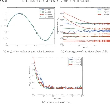
• pCN Algorithms 5.1 and 5.2 are implemented withβ = 0.6, and 106iterations. The results of the DKL optimization phase of the problem, using the Robbins– Monro Algorithm 4.1, appear in Figure 4. This figure shows the convergence ofmn in the rank 2 case; the convergence of the eigenvalues ofB for ranks 2, 4, and 6; and the minimization ofDKL. We only present the convergence of the mean in the rank 2 case, as the others are quite similar. At the termination of the Robbins–Monro step, theBn matrices are
Bn =
0.0857 0.00632
− 0.105
, (6.9)
Bn =
⎛ ⎜ ⎜ ⎝
0.0864 0.00500 −0.00791 −0.00485
− 0.106 0.00449 −0.00136
− − 0.0699 −0.000465
− − − 0.0739
⎞ ⎟ ⎟ ⎠, (6.10)
Bn =
⎛ ⎜ ⎜ ⎜ ⎜ ⎜ ⎜ ⎝
0.0870 0.00518 −0.00782 −0.00500 −0.00179 −0.00142
− 0.106 0.00446 −0.00135 0.00107 0.00166
− − 0.0701 −0.000453 −0.00244 9.81×10⁻⁵
− − − 0.0740 −0.00160 0.00120
− − − − 0.0519 −0.00134
− − − − − 0.0523
⎞ ⎟ ⎟ ⎟ ⎟ ⎟ ⎟ ⎠ . (6.11)
Note there is consistency as the rank increases, and this is reflected in the eigenvalues of theBn shown in Figure 4. As in the case of the scalar problem, more iterations of Robbins–Monro are computed than are needed to ensure convergence.
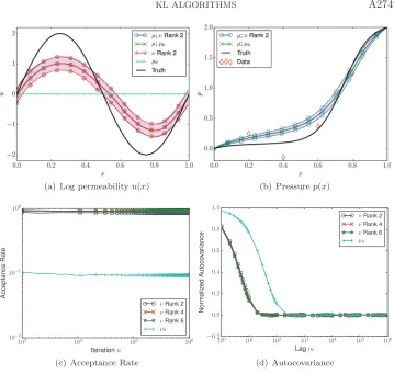
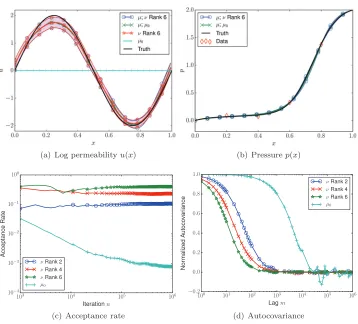
The posterior sampling, by means of Algorithms 5.1 and 5.2, is described in Figure 5. There is good posterior agreement in the means and variances in all cases, and the low rank priors provide not just good means but also variances. This is reflected in the high acceptance rates and low auto covariances; there is approximately an order of magnitude in improvement in using Algorithm 5.2, which is informed by the best Gaussian approximation, and Algorithm 5.1, which is not.
0.0 0.2 0.4 0.6 0.8 1.0
x
−1.5
−1.0
−0.5 0.0 0.5 1.0 1.5
mn
n=100
n=1000
n=10000
n=100000
(a)mn(x) for rank 2 at particular iterations
102 103 104 105
Iterationn
0.04 0.06 0.08 0.10 0.12 0.14 0.16
Eigen
values
of
Bn
νRank 2
νRank 4
νRank 6
(b) Convergence of the eigenvalues ofBn
100 101 102 103 104 105 Iterationn
20 25 30 35 40 45 50
DKL
[
mn ,Bn
]
+
Constant
νRank 2
νRank 4
νRank 6
(c) Minimization ofDKL
Fig. 4. Convergence of the Robbins–Monro Algorithm 4.1 applied to the Bayesian inverse
problem. (a)shows the convergence ofmnin the case of rank2, while(b)shows the convergence of the eigenvalues ofBnfor ranks2,4and6. (c)shows the minimization ofDKL. The observational
noise isγ = 0.1. The figures indicate that rank2 has converged after102 iterations; rank4 has
converged after103 iterations; and rank6has converged after104 iterations.
However, notice in Figure 5 that the posterior, even when±one standard devi-ation is included, does not capture the truth. The results are more favorable when we consider the pressure field, and this hints at the origin of the disagreement. The values at x= 0.2 and 0.4, and to a lesser extent at 0.6, are dominated by the noise. Our posterior estimates reflect the limitations of what we are able to predict given our assumptions. If we repeat the experiment with smaller observational noise,γ= 0.01 instead of 0.1, we see better agreement, and also variation in performance with respect to approximations of different ranks. These results appear in Figure 6. In this smaller noise case, there is a two order magnitude improvement in performance.
6.2. Conditioned diffusion process. Next, we consider measure μ given by
(1.1) in the case whereμ0is a unit Brownian bridge connecting 0 to 1 on the interval (0,1), and
Φ = 1
4ε2
1
0
1−u(t)2 2
dt,
a double well potential. This also has an interpretation as a conditioned diffusion [29]. Note thatm0=t andC0−1=−12 d2
dt2 withD(C −1
0 ) =H2(I)∩H01(I) withI= (0,1).
[image:17.612.75.429.76.414.2](a) Log permeabilityu(x) (b) Pressurep(x)
103 104 105 106
Iterationn
10−2
10−1
100
Acceptance
Rate
νRank 2
νRank 4
νRank 6
μ0
(c) Acceptance Rate
100 101 102 103 104 105 106 Lagm
−0.2 0.0 0.2 0.4 0.6 0.8 1.0
Nor
maliz
ed
A
utoco
var
iance
νRank 2
νRank 4
νRank 6
μ0
(d) Autocovariance
Fig. 5. Behavior of MCMC Algorithms 5.1 and 5.2 for the Bayesian inverse problem with
observational noiseγ= 0.1. The true posterior distribution,μ, is sampled usingμ0(Algorithm5.1)
and ν, with ranks2, 4and 6 (Algorithm5.2). The resulting posterior approximations are labeled
μ; μ0 (Algorithm 5.1) andμ; ν rank 2, (Algorithm5.2). The notationμ0 and ν rank K is used
for the prior and best Gaussian approximations of the corresponding rank. The distributions of
u(x), in(a),for the optimizedν rank2and the posteriorμoverlap, but are still far from the truth. The results for ranks 4and 6 are similar. (c)and (d)compare the performance of Algorithm5.2
when using ν rank K for the proposal, withK = 2,4, and6, against Algorithm 5.1. ν rank 2
gives an order of magnitude improvement in posterior sampling overμ0. There is not significant
improvement when usingνranks4and6over using rank2. Shaded regions enclose±one standard deviation.
We seek the approximating measureν in the formN(m(t), C) with (m, B) to be varied, where
C−1=C0−1+21 ε2B
andBis either constant,B∈R, orB :I→Ris a function viewed as a multiplication operator. Here, the eigenvalues of the covariance operator decay likej−2.
We examine both cases of this problem, performing the optimization, followed by pCN sampling. The results were then compared against the uninformed prior, μ0 =N(m0, C0). For the constantB case, no preconditioning on B was performed, and the initial guess was B = 1. For B =B(t), a Tikhonov–Phillips regularization was introduced,
(6.12) DαKL=DKL+α
2
˙
B2dt, α= 10−2.
[image:18.612.78.437.75.416.2](a) Log permeabilityu(x) (b) Pressurep(x)
103 104 105 106
Iterationn
10−4
10−3
10−2
10−1
100
Acceptance
Rate
νRank 2
νRank 4
νRank 6
μ0
(c) Acceptance rate
100 101 102 103 104 105 106 Lagm
−0.2 0.0 0.2 0.4 0.6 0.8 1.0
Nor
maliz
ed
A
utoco
var
iance
νRank 2
νRank 4
νRank 6
μ0
(d) Autocovariance
Fig. 6. Behavior of MCMC Algorithms 5.1 and 5.2 for the Bayesian inverse problem with
observational noise γ= 0.01. Notation as in5. The distribution ofu(x), shown in (a), for both the optimized rank 6 ν, and the posterior μoverlap, and are close to the truth. Unlike the case of γ = 0.1, (c) and (d)show improvement in using ν rank 6 within Algorithm 5.2, over ranks2
and 4. However, all three cases of Algorithm5.2are at least two orders of magnitude better than Algorithm5.1,which uses onlyμ0. Shaded regions enclose±one standard deviation.
For computing the gradients (4.6) and estimatingDKL,
DmΦ(v+m) =21
ε2(v+m)[(v+m)2−1], (6.13a)
DBΦν0(v) =
1 4ε2
1
0 v2dt, B constant, 1
4ε2v2, B(t). (6.13b)
No preconditioning is applied for (6.13b) in the case that B is a constant, while in the case thatB(t) is variable, the preconditioned gradient inB is
−αdtd22
−1
(Eν0(Δ
0DθΔ0)−Eν0(Δ
0)Eν0(D
θΔ0)) +B.
Because of the regularization, we must invert−d2/dt2, requiring the specification of boundary conditions. By a symmetry argument, we specify the Neumann boundary condition, B(0) = 0. At the other endpoint, we specify the Dirichlet condition B(1) =V(1) = 2, a “far field” approximation.
[image:19.612.78.436.90.414.2]0.0 0.2 0.4 0.6 0.8 1.0
x
0.0 0.2 0.4 0.6 0.8 1.0 1.2
mn
n=100
n=1000
n=10000
n=100000
(a)mn(t) at particular iterations
102 103 104 105
Iterationn
1 2 3 4 5 6 7 8
Bn
(b)Bnversusn.
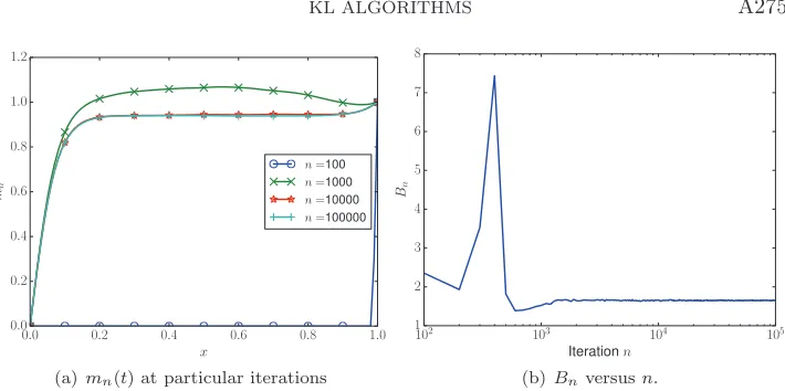
Fig. 7. Convergence of the Robbins–Monro Algorithm4.1applied to the conditioned diffusion
problem in the case of constant inverse covariance potentialB. (a)shows evolution ofmn(t)with
n;(b)shows convergence of theBnconstant.
The common parameters used are
• the temperatureε= 0.05;
• there were 99 uniformly spaced grid points in (0,1);
• as the endpoints of the mean path are 0 and 1, we constrained our paths to lie in [0,1.5];
• B and B(t) were constrained to lie in [10−3,101], to ensure positivity of the spectrum;
• the standard second order centered finite difference scheme was used forC0−1;
• trapezoidal rule quadrature was used to estimate 01m˙2 and 01B˙2dt, with second order centered differences used to estimate the derivatives;
• m0(t) =t,B0= 1,B0(t) =V(1), the right endpoint value;
• 105iterations of the Robbins–Monro algorithm are performed with 102 sam-ples per iteration;
• a0= 2 andan=a0n−3/5;
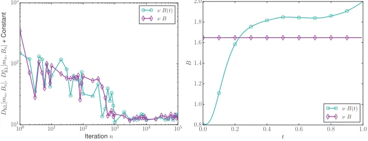
• pCN Algorithms 5.1 and 5.2 are implemented withβ = 0.6, and 106iterations. Our results are favorable, and the outcome of the Robbins–Monro Algorithm 4.1 is shown in Figures 7 and 8 for the additive potentialsB and B(t), respectively. The means and potentials converge in both the constant and variable cases. Figure 9 confirms that in both cases,DKLandDα
KLare reduced during the algorithm.
The important comparison is when we sample the posterior using these as the proposal distributions in MCMC Algorithms 5.1 and 5.2. The results for this are given in Figure 10. Here, we compare both the prior and posterior means and variances, along with the acceptance rates. The means are all in reasonable agreement, with
the exception of the m0, which was to be expected. The variances indicate that
the sampling done using μ0 has not quite converged, which is why it is far from
the posterior variances obtained from the optimized ν’s, which are quite close. The optimized prior variances recover the plateau betweent= 0.2 tot= 0.9, but could not resolve the peak near 0.1. VariableB(t) captures some of this information in that it has a maximum in the right location, but of a smaller amplitude. However, when one standard deviation about the mean is plotted, it is difficult to see this disagreement in variance between the reference and target measures.
[image:20.612.80.435.76.253.2]0.0 0.2 0.4 0.6 0.8 1.0
x
0.0 0.2 0.4 0.6 0.8 1.0 1.2
mn
n=100
n=1000
n=10000
n=100000
(a)mn(t) at particular iterations.
0.0 0.2 0.4 0.6 0.8 1.0
x
0 1 2 3 4 5 6
Bn
n=100
n=1000
n=10000
n=100000
(b)Bn(t) at particular iterations.
Fig. 8. Convergence of the Robbins–Monro Algorithm4.1applied to the conditioned diffusion
problem in the case of variable inverse covariance potentialB(t). (a)showsmn(t)at particular n.
(b)showsBn(t)at particular n.
100 101 102 103 104 105 Iterationn
101
102
103
DKL
[
mn ,Bn
]
,D
α[KL mn ,Bn
]
+
Constant
ν B(t)
ν B
0.0 0.2 0.4 0.6 0.8 1.0
t
0.8 1.0 1.2 1.4 1.6 1.8 2.0
B
ν B(t)
ν B
Fig. 9.Minimization ofDα
KL(forB(t)) andDKL(forB) during Robbins–Monro Algorithm4.1
for the conditioned diffusion problem. Also plotted is a comparison ofBandB(t)for the optimized
ν distributions.
In Figure 11 we present the acceptance rate and autocovariance, to assess the performance of Algorithms 5.1 and 5.2. For both the constant and variable potential cases, there is better than an order of magnitude improvement overμ0. In this case, it is difficult to distinguish an appreciable difference in performance between B(t) andB.
7. Conclusions. We have demonstrated a viable computational methodology
for finding the best Gaussian approximation to measures defined on a Hilbert space of functions, using the KL divergence as a measure of fit. We have parameterized the covariance via low rank matrices, or via a Schr¨odinger potential in an inverse co-variance representation, and represented the mean nonparametrically, as a function; these representations are guided by knowledge and understanding of the properties of the underlying calculus of variations problem as described in [28]. Computational results demonstrate that, in certain natural parameter regimes, the Gaussian approx-imations are good in the sense that they give estimates of mean and covariance which are close to the true mean and covariance under the target measure of interest, and
[image:21.612.82.435.97.254.2] [image:21.612.77.436.309.447.2]