Parameterized complexity : permutation patterns, graph arrangements, and matroid parameters

(1)

A Thesis Submitted for the Degree of PhD at the University of Warwick

http://go.warwick.ac.uk/wrap/77519

This thesis is made available online and is protected by original copyright. Please scroll down to view the document itself.

(2)

Permutation Patterns, Graph Arrangements,

and Matroid Parameters

by

Luk´

aˇs Mach

Thesis

Submitted in partial fulfilment of the requirements

for the degree of

Doctor of Philosophy

(3)

Acknowledgements

I am grateful to my supervisor, Dan Kr´al’, for all the opportunities, support, and

guidance provided during my doctoral studies. The feedback provided by my

viva examiners, Graham Cormode and Daniel Paulusma, is greatly appreciated.

I want to thank all the researchers who have co-authored a paper with me:

Ivan Bliznets, Marek Cygan, Frantiˇsek Kardoˇs, Pavel Klav´ık, Pawe l Komosa,

Dan Kr´al’, Anita Liebenau, Andrej Mikul´ık, Micha l Pilipczuk, Jean-Sebastien

Sereni, and Tom´aˇs Toufar. My bachelor students at Charles University in Prague,

Adam Dominec and Viktorie V´aˇsov´a, were great collaborators as well.

I happily acknowledge the support provided by the following organizations:

Computer Science Institute of Charles University in Prague, the Grant Agency

of Charles University (GAUK), University of Warwick, the Centre for Discrete

Mathematics and its Applications (DIMAP) at Warwick, University of Warsaw,

and the Warsaw Center of Mathematics and Computer Science (WCMCS).

Dur-ing my studies, I have received support from the European Research

Coun-cil under the European Union’s Seventh Framework Programme

(FP7/2007-2013)/ERC grant agreement no. 259385 and from the student project GAUK

no. 592412.

I want to thank all the great people and friends I have met before and

during my studies at Warwick, in particular Rafael Barbosa, Martin B¨ohm,

(6)

Michail Fasoulakis, Matthew Felice-Pace, Tereza Hulcov´a, Marcin Jurdzinski,

Tereza Klimoˇsová, Matjaˇz Krnc, Lukáˇs Lánský, Bernard Lidický, Felix Ling,

Jirka Matˇejka, Nick Matsakis, Ta´ısa Martins, Lukáˇs Novotný, Adéla Peterová,

Jakub Polonsk´y, Jakub Sliacan, Vojta T˚uma, Danuˇse Vavˇrinov´a, Honza Volec,

and Nick Zervoudis.

I would like thank to my family, especially my mother, father, and brother,

(7)

Declarations

The majority of this thesis is based on results that are either already published or

whose publication is currently in preparation. Below, we list these publications

including submitted papers (and papers in preparation). The thesis is divided

into seven chapters:

Chapter 1 gives an overview of the obtained results and a commentary on how they relate to the current state of the art in computer science.

Chap-ter 2 provides the reader with background maChap-terial of the relevant areas and

fixes notation used throughout the text. This notation and the statements

of definitions, lemmas, hypotheses, and theorems from this chapter are

of-ten identical or similar to those used in one of the standard introductory

monographs referenced in the text.

Chapter 3 is based on the result [5]. This collaboration with Ivan Bliznets,

Marek Cygan, and Pawe l Komosa has been published in Information

Pro-cessing Letters.

The results presented in Chapter 4 are a joint work [6] with Ivan Bliznets,

Marek Cygan, Pawe l Komosa, and Micha l Pilipczuk. They were accepted

for presentation at the SODA 2016 conference.

Chapter 5 is a joint work with Tom´aˇs Toufar. The corresponding article [64]

(8)

is a contribution to the8th International Symposium on Parameterized and

Exact Computation (IPEC 2013), where it has been awarded the IPEC

Excellent Student Paper award. The results of this chapter overlap

signifi-cantly with the Bachelor thesis of Tom´aˇs Toufar.

In Chapter 6, we study the algorithmic aspects of the matroid branch-depth

parameter. These results were obtained together with Frantiˇsek Kardoˇs,

Daniel Kr´al’, and Anita Liebenau. The corresponding paper [52]

(submit-ted for a journal publication) introduces this parameter and gives both

structural and algorithmic theorems.

Conclusion of the work with some indication of possible future research

directions is given in Chapter 7.

With the exception of the contents of Chapter 5 (mentioned above), no result of

this thesis already appeared in another academic thesis. The scientific

contribu-tion of the individual authors of the above results is roughly proporcontribu-tional to the

number of authors of each result. This thesis has not been previously submitted

(9)

Abstract

The theory of parameterized complexity is an area of computer science focusing

on refined analysis of hard algorithmic problems. In the thesis, we give two

complexity lower bounds and define two novel parameters for matroids.

The first lower bound is a kernelization lower bound for the Permutation Pattern Matching problem, which is concerned with finding a permutation

pattern inside another input permutation. Our result states that unless a

cer-tain (widely believed) complexity hypothesis fails, it is impossible to construct a

polynomial time algorithm taking an instance of the Permutation Pattern Matching problem and producing an equivalent instance of size bounded by a

polynomial of the length of the pattern. Obtaining such lower bounds has been

posed by St´ephane Vialette as an open problem.

We then prove a subexponential lower bound for the computational

com-plexity of the Optimum Linear Arrangement problem. In our theorem, we

assume a conjecture about the computational complexity of a variation of the

Min Bisection problem.

The two matroid parameters introduced in this work are called

amalgam-width and branch-depth. Amalgam-amalgam-width is a generalization of the branch-amalgam-width

parameter that allows for algorithmic applications even for matroids that are not

finitely representable. We prove several results, including a theorem stating that

deciding monadic second-order properties is fixed-parameter tractable for

gen-eral matroids parameterized by amalgam-width. Branch-depth, the other newly

introduced matroid parameter, is an analogue of graph tree-depth. We prove several statements relating graph tree-depth and matroid branch-depth. We also

present an algorithm that efficiently approximates the value of the parameter on

a general oracle-given matroid.

(10)

Chapter 1 Introduction

Efficient computation is one of the main focal points of computer science. Since

the beginnings of the field, researchers have attempted to either find algorithms

minimizing resources exerted for obtaining the correct answer to algorithmic

problems or to find negative results – reasons why some problems should not

admit algorithms above certain levels of efficiency. The first theoretical notion

trying to characterize what is practically computable was the class P of

algo-rithmic problems solvable in polynomial number of steps. From a practical

standpoint, this mathematical formalization has several major issues. One

par-ticular is that many algorithmic problems widely believed to lie outside of P are

actually routinely solved in the real world, e.g. by CSP-solvers. The instances

encountered as a result of real applications sometimes seem to posses certain

structural properties that help to accelerate the computation. A more detailed

look at the (conjectured) land behind the boundaries of Pis certainly warranted.

Parameterized complexity, the area to which this thesis mainly contributes,

provides a framework for such refined analysis. In this field, the set of all possible

inputs of an algorithmic problem (e.g., the set of all graphs) is divided into an

(11)

infinite number of layers by equipping the individual instances with a

parame-ter value. Different parameterizations of the same set of inputs are sometimes

sensible. Ideally, the parameter should, roughly speaking, correspond to the

al-gorithmic difficulty of resolving the instance. One of the main aims of the area

is to obtain fixed-parameter tractable (FPT) algorithms for parameterized

prob-lems. These are algorithms with the running time of O f(k)·nc

, where f(·) is a computable function,n the size of the input of the instance, k the value of the parameter, and ca real constant.

An example of a parameterization is given by the classical notion of graph

tree-width, employed prominently in the proof of the Robertson-Seymour

theo-rem (see, e.g., [76]). The tree-width of a graph is a value proportional to the

“distance” the graph is from being a tree (or a forest). Graphs with tree-width 1

are actually precisely forests. The formal definition is given as Definition 8 in

Section 2.3. A large number of difficult (NP-hard) problems on graphs are easy

to solve on graphs of bounded tree-width: for any choice of a constant k, there exists a polynomial algorithm solving the problem for graphs of tree-width at

mostk. Many of the corresponding algorithms are FPTunder this parameteriza-tion. A classical result of Courcelle [21] generalizes this to all decision problems

expressible as formulas in monadic second-order logic.

Theorem 1 (Courcelle, [21]). Let ϕ be a fixed formula in monadic second-order logic andk ∈N. Then, there is an algorithm deciding whether a graphGsatisfies

ϕ in linear time for graphs of tree-width at most k.

Parameterized complexity also provides us with the first formal framework to

theoretically analyze preprocessing algorithms through the notion of

(12)

a problem to an equivalent instance of strictly smaller size. Such algorithms are

useful when it comes to solving difficult problems in practice: an efficient

prepro-cessing algorithm is applied exhaustively after which another approach is used to

solve the reduced instance. Obviously, it is desirable for the size of the reduced

instance to be as small as possible. We say that a parameterized problem has

a kernel if there exists a polynomial time preprocessing algorithm guaranteed to

produce an instance of size and parameter value bounded by a function of the

parameter of the initial instance. Such algorithm is then called a kernelization

algorithm. Conveniently, the class of FPT problems and the class of problems

with a kernel coincide [27]. A stronger notion is represented by the class of

problems with a polynomial kernel. For these, there is a kernelization algorithm

always producing an instance of size bounded by a polynomial of the parameter

value of the initial instance.

The first result of this thesis is a kernel size lower bound for thePermutation

Pattern Matching problem. A permutation π contains a permutation σ as

a pattern if it contains a subsequence of length |σ| whose elements are in the same relative order as in the permutation σ. The Permutation Pattern Matching problem is the corresponding algorithmic problem. The standard

parameterization is by |σ|. Guillemot and Marx [39] recently resolved the issue of whether the problem is in FPTaffirmatively, implying that the problem has a

kernel. Vialette [82] asked for lower bounds on the size of this kernel. We prove

the following:

Theorem 2. Unless NP ⊆ co-NP/poly, the Permutation Pattern Match-ing problem does not have a polynomial kernel.

(13)

in the field of computational complexity and one of the typical starting points

for obtaining kernelization lower bounds. Its failure would imply the collapse of

the polynomial hierarchy to the third level. Consequently, there is a high degree

of confidence in its validity within the research community. The proof of this

theorem is given in Chapter 3.

A lower bound of a different kind is presented in Chapter 4, where we are

concerned with the standard (i.e., non-parameterized) _{Optimum Linear}

Ar-rangement problem. We prove a hardness result relative to the computational

complexity of the gap version of theMin Bisection problem. (The precise

def-initions of these algorithmic problems are deferred to Chapter 4.) Specifically,

we formulate the following conjecture:

Conjecture 3. There exist d0 ∈ N and α, β ∈ (0,1), α < β such that for each

d≥d0 there is no 2o(n) time algorithm for (d, α, β)-Gap Min Bisection.

The (d, α, β)-_{Gap Min Bisection}problem is defined in Chapter 4. Essentially, it is a gap version of the Min Bisection problem on regular graphs. The

mo-tivation for this conjecture is given in Chapter 4. There, we prove the theorem

below.

Theorem 4. Unless Conjecture 3 fails, there is no 2o(n+m) _{time algorithm for}

Optimum Linear Arrangement, where n is the number of vertices of the

input graph and m the number of its edges.

This is a similar kind of computational complexity bound to those based

on the Exponential Time Hypothesis (ETH), which stipulates that there is no

algorithm for theq-SATproblem running in 2o(n) time, wherenis the number of

(14)

reported in [6] we prove complexity lower bounds for several graph completion

problems first under the ETH and then apply Conjecture 3 and Theorem 4 to

substantially strengthen them.

Let us briefly comment on some results from [6] that are not part of this

thesis. Hopefully, they provide additional level of justification for our conjecture

and illuminate the relevance of Theorem 4. Graph completion problems are

algo-rithmic problems where the question to be decided is whether a certain number

of edges can be added to the input graph in such a way that the resulting graph

belongs to some class, e.g., the class of chordal graphs. We consider the natural

parameterization of these problems by the number of edges to be added and give

the following bounds. (We refer the reader to Section 2.4 for the definitions of

the algorithmic problems in question.)

Theorem 5 (Bliznets et al., [6]). Unless the ETH fails, there exists c > 0 such that none of the following problems has a 2O(k14/logc_k₎

·nO(1) algorithm, where k

is the value of the parameter and n is the input size: Chordal Completion, Trivially Perfect Completion, Proper Interval Completion, and

Interval Completion.

The parameterized problems from the above theorem have been studied

exten-sively in the literature [34]. Theorem 4 allows us to obtain lower bounds that

essentially match the fastest presently known parameterized algorithms.

Theorem 6 (Bliznets et al., [6]). Unless Conjecture 3 fails, for all ε > 0 there is no 2O(

√ k1−ε₎

·nO(1) algorithm for any of the following problems: Chordal Completion, Trivially Perfect Completion, Proper Interval

(15)

For example, the currently fastest known parameterized algorithm for _Chordal

Completionruns in 2O( √

klogk)₊_nO(1) _{steps [34].}

In Chapter 5, we introduce the notion of amalgam-width. This is an attempt

to generalize the notion of width parameters to matroids. Several such

param-eters have already been introduced in the literature, including a direct

general-ization of tree-width [44] and clique-width [22]. However, our aim is to obtain

one that allows the algorithmic applications even for non-representable matroids.

Furthermore, amalgam-width has the nice property that it corresponds to a

nat-ural, standard gluing operation called amalgamation. We prove the following

theorem:

Theorem 7. For eachk ∈N and each formulaϕ in monadic second-order logic there is an algorithm deciding whether a matroid M satisfiesϕ in linear time for matroids of amalgam-width bounded from above byk (assuming the corresponding amalgam decompositionT of the matroid is given explicitly as a part of the input).

Amalgam-width generalizes a parameter based on 2-sums introduced in [81]

and branch-width for matroids representable over finite fields. The later

gener-alization is in the sense that amalgam-width can be bounded by a function of

branch-width. The proof of this claim (Proposition 46) is constructive and leads

to an efficient algorithm constructing such amalgam decompositions.

The next chapter introduces another matroid parameter, the matroid

branch-depth. This time, the main motivation for our algorithmic results is structural.

The parameter is a matroid analogue of graph tree-depth, an established graph

parameter used among others by Neˇsetˇril and Ossona de Mendez in their research

on combinatorial limits [66]. There, the notion of tree-depth is used to constrain

(16)

a combinatorial limit called modeling can be guaranteed. In [52] we extend

this theory to matroids by introducing matroid modelings, the branch-depth

parameter, and the notion of first-order convergent sequences of matroids. Apart

from a number of negative results, we also prove a theorem analogous to the

abovementioned result on graphs. Specifically, we show that every first-order

convergent sequence of matroids with bounded branch-depth representable over

a finite field has a matroid modeling. The similarity between this statement and

the aforementioned result of [66] indicates that at least from some perspective

the branch-depth parameter is an analogous notion to tree-depth.

In Chapter 6 of this thesis, we focus exclusively on the algorithmic aspects of

the branch-depth parameter and on its relationship with tree-depth. We provide

an efficient algorithm approximating the parameter value for any oracle given

matroid. The close relation with tree-depth is substantiated by the following

properties:

The branch-depth of a graphic matroid M(G) is at most the tree-depth

of G. Furthermore, it can be bounded from below by a function of the tree-depth if G is 2-connected.

Both branch-depth and tree-depth are minor monotone parameters.

The branch-depth of a matroid is at most the square of the length of its largest circuit (recall that the tree-depth of a graphGis at most the length of its longest path).

The branch-depth of a matroid is at least the logarithm of the length of

(17)

The branch-depth parameter is defined through a particular kind of

(18)

Chapter 2 Preliminaries

In this chapter, we review the notation adopted by this thesis and reference results

from literature utilized in the proofs of the subsequent chapters. The contents

are not intended as an introductory text to the field. Rather, we hope to provide

a sufficient amount of context for our results while maintaining brevity. Many

of the elementary notions are mentioned simply to fix the notation. We refer

the reader to the monographs [25] and [71] for a comprehensive introduction to

graph theory and the theory of matroids, respectively. Parameterized algorithms

are treated in the recent book [23].

2.1 Basic notation

The set {i, i+ 1, . . . , j−1, j} is denoted by [i, j]. We let [n] := [1, n]. The set of all subsets of the set X is denoted by S(X) and X_r is the set of all subsets of X of size r ∈ N. For a function f and a set X we define f(X) to be the set

{f(x) :x∈X}. For a matrixM, the element in thei-th row and thej-th column is denoted by Mi,j. A submatrix of a matrix M is a matrix obtained by deleting

(19)

some rows and/or columns of M. For a non-empty set Σ, we denote by Σ∗ the set of all sequences of finite length composed of elements from Σ. For example

{0,1}∗ _{is the set of all finite binary strings. A formula in} _{conjunctive normal}

form (CNF) is a formula C1 ∧C2 ∧. . .∧Ck, where Ci are clauses of the form

Ci =ì1∨ì2∨. . .∨ìki, whereìj is a literal (either a variable or a negated variable).

This formula is a q-CNF formulaif all its clauses have precisely q literals.

2.2 Permutations

A permutationπis a bijection from [n] to [n]. The valueπ(i) is calledthe entry of

π at positioni(orindexi). We use|π|to denote the size of the domain ofπ. Two common representations of a permutation π are used in the thesis: the vector (π(1), π(2), . . . , π(n)) and the corresponding permutation matrix. The latter is a

|π| × |π| binary matrix with 1-entries precisely on coordinates (π(i), i).

2.3 Graphs

A graph is a pair (V, E), where V is the set of vertices and E ⊆ V₂

is the set of

edges. Therefore, unless otherwise specified, graphs in this thesis are undirected,

loopless, and without edge multiplicities. In line with common practice, an edge

e={u, v} is denoted by (u, v) although the pair is not ordered. We say that an edge e is incident with the vertex v if v ∈e. The set of vertices of G is denoted

V(G) whileE(G) is its edge-set. A hypergraphis a pair (V, E), whereE ⊆ S(V). An r-uniform hypergraphis a hypergraph whereE ⊆ V_r

. Therefore, the notions

of a graph and a 2-uniform hypergraph coincide. A graph H is a subgraph of G

(20)

E(H) =E(G)∩ V(₂H)

. We use G[X] to denote an induced subgraph of G with vertex set X. A complete graph Kn on n vertices is the graph (V, V₂

), where

V = [n]. A graph G contains a clique of size l if an isomorphic copy of Kl is

a subgraph of G.

For a vertex v, deg(v) is its degree: the number of edges incident with v. We say that a graph is d-regular if all its vertices have degree d. We use ∆(G) := max{deg(v) : v ∈V(G)} to denote the maximum degree of G. The set N(v) :=

{w : (v, w) ∈ E(G)} is the neighbourhood of v. This notation is extended to subsets of vertices X, i.e. N(X) = S

v∈XN(v)\X.

If X, Y ⊆ V are disjoint, then E(X, Y) is the set of edges between X and

Y. We use G[X, Y] to denote the induced bipartite subgraph of G with parts

X and Y. That is, G[X, Y] is the graph with vertex set X∪Y that contains precisely the edges E(X, Y). For X ⊆ V, we denote by δ(X) the set of edges with exactly one endpoint in X. A bipartition of a graph G is a pair (A, B), where A, B ⊆ V(G), A∩B = ∅, and A∪B = V(G). A balanced bipartition of a graph G is a bipartition (A, B) such that |A| − |B|

≤ 1. We define a cut as

the set of edges E(A, B), for a bipartition (A, B) of V. A balanced cut is the set

E(A, B) where (A, B) is balanced bipartition. The number |E(A, B)| is called the size of the cut. A complement of G is the graph with the vertices V and edges V₂\E. We denote it byG. We add subscripts to the above notation, e.g., deg_G(v), NG(X), δG(X), or EG(U, V), when it is not clear from context which

graph we refer to.

(21)

not a part of the edge-set of the cycle. An interval graphis a graphG such that

V(G) can be placed in correspondence to a set of intervals on the real line and two vertices are connected precisely when they have a non-empty intersection. (We

also use the terminterval graph for graphs isomorphic to such graphs.) A proper

interval graphis an interval graph where no pair of vertices corresponds to a pair

of intervals such that one properly contains the other. A trivially perfect graph

is an interval graph where each pair of vertices corresponds to a pair of intervals

that are either disjoint or one contains the other.

A k-tree is either a clique of size k+ 1 or a graph that can be obtained from a smallerk-tree by adding a new vertex and connecting it tok vertices that already form a clique.

Definition 8. Tree-width of a graph G is the least number k ∈ N such that G

is a subgraph of a k-tree.

2.4 Algorithms

Formally, an algorithmic problem is a mapping f :{0,1}∗ _{→ {}₀_,₁_}∗ _prescribing

each binaryinputthe appropriateoutput. We are interested in the construction of

Turing machines encoding the function f while simultaneously satisfying certain requirements, typically on running time. Such a Turing machine (and the

corre-spondingalgorithm) is said to solvethe particular problemf. Complementarily, we sometimes try to find reasons why a Turing machine with certain

proper-ties should not exist. For those arguments, additional hypotheses are typically

(22)

A decision problem is a special kind of algorithmic problem where the set

of values of the mapping is simply {0,1}. The instances mapping to 1 are sometimes termed the “YES” instances, while the rest are “NO” instances. A

decision problem can be identified with the subset of inputs {0,1}∗ _{where the}

mapping f from the above definition attains the value of 1. Such a set is often called a language. We say that the Turing machine solving the decision problem

in questionrecognizesthis set. Since this thesis is not concerned with the low-level

implementation details of Turing machines, we abuse the notation and identify

the finite binary sequences with the discrete structures (graphs, permutations,

formulas, subsets of vertices, etc.) they are representing. The particular choice

of representation is almost never an issue as long as it is reasonably efficient.

We now give an overview of the algorithmic problems that appear in this

thesis. _SAT,_Clique, and_{Dominating Set}are well knownNP-hard problems:

SAT

Input: A formulaϕin the conjunctive normal form.

Question: Is there an assignment of values to the free variables ofϕsatisfying the formula?

Clique

(23)

Dominating Set

Input: A graphG= (V, E), an integer k.

Question: Does G contain a dominating set of size k?

There are many variations on the SAT problem in the literature. Of particular

importance is the q-SAT problem, where q ∈N.

q-SAT

Input: A formula ϕ in the conjunctive normal form where each clause con-tains q distinct literals.

Question: Is there an assignment of values to the free variables of ϕ satis-fying the formula?

Graph completion problems are a particular type of decision problems where

we ask whether a number of edges can be added to an input graph so that the

resulting graph belongs to a certain class of graphs, e.g., chordal graphs. The

following completion problems areNP-hard. Their parameterized variants (where

k is the parameter) are inFPT.

Chordal Completion

Input: A graphG, an integer k.

Question: Can k edges be added to G so that Gis a chordal graph?

Trivially Perfect Completion

(24)

Proper Interval Completion

Question: Can kedges be added toGso thatGis a proper interval graph?

Interval Completion

Question: Can k edges be added to G so that Gis an interval graph?

2.5 Complexity classes

A complexity class is a (typically infinite) set of decision problems. The two

most fundamental complexity classes are P and NP. The former is the set of all

decision problems solvable by a Turing machine in polynomial time. The latter

is a set of decision problems that can be decided in polynomial time when an

appropriate certificate (i.e., an appropriate input dependent string of bits with

polynomial length) is given to the Turing machine in addition to the input. If C

is a complexity class, then co-C is the class

n

{0,1}∗ \X :X ∈C

o

.

For example, co-NP is the class of all problems, where the “NO” instances can

be identified in polynomial time when an appropriate certificate is provided.

Deciding a problem in NP is equivalent to determining if there exists a

poly-nomially long string of bits satisfying a certain property from P. When resolving

(25)

P holds for all such strings. This leads to a method that takes a class of

prob-lems and generates a definition of a new complexity class. Iterating this gives us

the polynomial hierarchy of complexity classes. Structural complexity is not the

focus of this thesis and we reference the polynomial hierarchy in only a limited

number of places to provide basic information about how certain conjectures fit

within the rest of the theory. We therefore omit the precise definition of the

hierarchy and only recall two key properties. Firstly, the base level of the

hier-archy consists of the class P with the next level being formed by NP and co-NP.

Secondly, any class from the hierarchy is a superset of each of the classes on the

levels beneath it. These inclusions are widely believed to be strict. The famous

P 6=NP conjecture corresponds to a strict inclusion between the first two levels

of the polynomial hierarchy.

We can also define a so called non-uniform class C/poly for each complexity class C. A decision problem L is in C/poly if there exists a set A ∈ C and an advice function g :N→ {0,1}∗ _{with the properties:}

1. there existsk ∈N such that|g(n)| ≤nk for all n∈N,

2. x∈L⇔(x, g(|x|))∈A.

2.6 Common hypotheses in complexity theory

The following two hypotheses are routinely assumed to hold in the area of

com-putational complexity:

Hypothesis 9. P6=NP.

(26)

Of course, Hypothesis 9 is the more likely answer to the central question of

computer science. Its failure would imply the collapse of the entire polynomial

hierarchy, something generally considered quite unlikely. Hypothesis 10 is slightly

stronger. Its failure would imply the collapse of the polynomial hierarchy to the

third level [20]. Still, even this stronger hypothesis is considered to be very safe

and is often used by researchers as a starting point from which complexity lower

bounds are derived. Yet another standard complexity hypothesis is discussed in

the following section.

2.7 Exponential Time Hypothesis

The trivial approach of solving the 3-SAT problem where the input formula ϕ

has n variables and m clauses uses O(m2n_{) steps.} _{Although some}

improve-ments on this are possible, the current state of research strongly suggests that

this exponential time complexity is unavoidable. This leads us to the following

hypothesis, which is called the Exponential Time Hypothesis (ETH) [49].

Exponential Time Hypothesis. The infimum of the set of constants c for which there exists an algorithm solving 3-SAT in time O∗(2cn) is strictly larger

than zero.

The ETH asserts that 3-SAT cannot be solved in 2o(n) time. (There is a

stronger variant of the ETH, calledthe Strong Exponential Time Hypothesis [50].

However, the confidence in its validity is significantly weaker than the confidence

in the ETH.)

As already mentioned in the previous chapter, the ETH can be employed to

(27)

algo-rithmic problems. Suppose there is an efficient reduction from 3-_SAT to some

decision problem Q. An algorithm solving Q “too quickly” would then violate the ETH. The precise lower bound on the runtime of any algorithm solving Q

obtained in this way depends on the properties of the reduction. Specifically,

we are concerned with the size of the instances of Qgenerated from an instance of 3-SAT with n variables. Reductions that are guaranteed to generate smaller

instances result in stronger bounds on the complexity of Q.

Two issues come into the picture. Firstly, there might be an inherent blow-up

in the size of the instances when reducing to Q. For example, a 3-SAT instance

with n variables and m clauses might require instances of Q of size at least n2. Secondly, we do not have exact knowledge of the number of clauses of the instance

of 3-SAT and thus can only assume m ≤ n3. Since polynomial reductions from

3-_SAT often explicitly encode the individual clauses of the formula, this could

again result in a weaker bound. Fortunately, the second problem can be dealt

with through the Sparsification Lemma:

Theorem 11 (Sparsification Lemma, [50]). For any ε > 0 and q > 0, there exists a constant C = C(ε, q) such that any q-CNF formula ϕ with n variables can be expressed as Vt

i=1ψi, where t≤2εn and each ψi is a q-CNF formula with

the same variable set as ϕand number of clauses bounded by Cn. Moreover, this formula can be constructed in O∗₍₂εn₎ _steps.

When combined, the Exponential Time Hypothesis and Sparsification Lemma

imply there is no 2o(n+m) _{algorithm for}

3-SAT. A reduction from 3-SATto some

decision problemQthat results in instances of size bounded from above byf(n+

m) therefore implies there are no algorithms recognizing Q in 2o(f−1₍_n₊_m₎₎

steps

(28)

2.8 Expanders

Expanders are sparse graphs that behave in a random-like manner. Their key

property is that if we look at any subset X of the vertex set of such a graph, we are guaranteed to see a lot of edges going between X and the remainder of the vertex set. In this work, expanders are used as a black box for a construction in

Chapter 4.

The Cheeger number h(G) of a graph G is the quantity

h(G) := min

_|

δ(X)|

|X| :X ⊆V(G),|X| ≤

|V(G)|

2

.

We say that a graph G is a (d, e)-expander if it is d-regular and has h(G) ≥ e. The following theorem provides us with an explicit construction of expander

graphs [45].

Theorem 12. For every primepand everyk ∈Nwe can construct in polynomial time (d,d−2

√ d−1

2 )-expanders, where d =p k_{+ 1.}

We use Gn,d to denote a d-regular expander graph on n vertices such that

h(G)≥ d

3.

The above theorem provides us with a polynomial deterministic algorithm

(29)

2.9 Parameterized complexity and kernelization

A parameterized problem is a set Q ⊆ Σ∗ ×N, where Σ is a fixed alphabet. The value k of the instance (x, k) ∈ Q is its parameter. A problem Q is in

FPT if there is an algorithm deciding (x, k)∈Qin time f(k)|x|O(1)_{, where} _f _{is a}

computable function. Similarly to the situation in “standard” complexity theory,

a hierarchy of classes of parameterized problems can be introduced along with

a suitable notion of fixed-parameter tractable reductions. One of such standard

hierarchies is the W-hierarchy, introduced by Downey and Fellows [27]:

FPT⊆W[1]⊆W[2]⊆. . .⊆W[P].

Similarly to the situation with the polynomial hierarchy discussed in Section 2.5,

we are not focusing on the structural aspects of parameterized complexity in

this work and the W-hierarchy is referenced only in a handful of places to pro-vide additional context. The reader is referred to [33] for a detailed structural

treatment of the theory of parameterized complexity, the precise definitions of

the above complexity classes, and the notion of fixed-parameter tractable

reduc-tions. For our work, the following properties of the hierarchy are relevant. The

above inclusions are conjectured to be strict. In fact, the ETH discussed in

Sec-tion 2.7 impliesFPT6=W[1]. TheCliqueproblem (parameterized by the size of

the clique) is complete for the class W[1], while the Dominating Set problem

(parameterized by the size of the dominating set) is complete for W[2].

Algorithms solving a decision problem are required to either output YES

or NO. This can be relaxed by not requiring the algorithm to output a definite

(30)

one that is as small as possible. This leads us to the notion of kernelization

algorithms, which we have already discussed in the previous chapter. Below, we

provide a rigorous definition.

Definition 13. A kernelization algorithm for a parameterized problem Q is an algorithm that given an instance (x, k)∈Σ∗×N produces in p(|x|+k) steps an instance (x0, k0) such that

1. (x, k)∈Q⇔(x0, k0)∈Q and

2. |x0|, k0 ≤f(k),

where p(·) is a polynomial and f(·) a computable function.

If there is a kernelization algorithm for Q, we say thatQ has a kernel. If the function f(·) in the above definition can be bounded by a polynomial, we say that Q has a polynomial kernel.

There is a simple relationship between the class FPT and problems with a

kernel given by the theorem below.

Theorem 14 (Theorem 1.39 in [33]). For every parameterized problem Q, the following are equivalent:

1. Q is in FPT.

2. Q is decidable and has a kernel.

A result of Bodlaender et al. [8], which builds on [7, 35], is often used to

de-rive kernelization lower bounds under the widely believed complexity assumption

(31)

We start a brief exposition of this standard machinery with two technical

definitions.

Definition 15 (Bodlaender et al., [8]). An equivalence relation R onΣ∗ is called a polynomial equivalence relation if the following two conditions hold:

1. There is an algorithm that given two strings x, y ∈ Σ∗ decides whether x

and y belong to the same equivalence class in (|x|+|y|)O(1) time.

2. For any finite set S∈Σ∗ the equivalence relation R partitions the elements of S into at most (maxx∈S|x|)O(1) equivalence classes.

An example of such a relation is the grouping of instances of the same size.

Definition 16 (Bodlaender et al., [8]). Let L ⊆ Σ∗ be a set and let Q ⊆ Σ∗ ×

N be a parameterized problem. We say that L cross-composes into Q if there is a polynomial equivalence relation R and an algorithm which, given t strings

x1, x2, . . . , xt belonging to the same equivalence class of R, computes an instance

(x∗, k∗)∈Σ∗×N in time polynomial in Pt

i=1|xi| such that:

1. (x∗, k∗)∈Q⇔xi ∈L for some 1≤i≤t,

2. k∗ is bounded by a polynomial in maxt

i=1|xi|+ logt.

As the following theorem states, widely believed complexity assumptions

im-ply that it is unlikely for anNP-hard problem to cross-compose into a

parameter-ized problem with a polynomial kernel. The reason behind this is that it would

then allow us to find a satisfiable instance of SAT among a very large set of

SAT-instances by dividing it in two halves, cross-composing the first half of the

instances, kernelizing the resulting instance, solving the resulting instance, and

(32)

Of course, the running time of this routine is not polynomial but the existence of

such a “detection” algorithm is still something that is generally considered very

unlikely for SAT.

Theorem 17 (Bodlaender et al., [8]). Let L⊆Σ∗ be an NP-hard language. If L

cross-composes into the parameterized problem Q and Q has a polynomial kernel then NP ⊆co-NP/poly.

2.10 Matroids

We now present the basic concepts and definitions of the theory of matroids.

A matroid M is a tuple (E,I) such that E is finite and I ⊆ S(E) is the set of independent sets ofM. The setIis not a general set system – rather, it is required to satisfy the following matroid axioms. Firstly,Iis not empty. Secondly, it must

contain as elements all subsets of any independent set (including the empty set).

Finally, the set I must satisfy the exchange axiom:

∀F, F0 ∈ I satisfying |F|<|F0| there is x∈F0 :F ∪ {x} ∈ I.

The set E is termed the ground set. For a general matroid M, we denote the ground set by E(M) and call its elements the elements of M. If a set is not independent, we call itdependent. Any minimal dependent set is calleda circuit.

The set of all circuits of the matroid, denoted by C(M), uniquely determines the matroid. Any maximal independent set is a basis of M. We note that while we only work with finite matroids in this thesis, there are generalizations of the

theory to infinite matroids [13].

(33)

that I ∈ I. The closure operator cl(F) acting on subsets of E(M) is defined as cl(F) :=

x : r(F ∪ {x}) = r(F) . It can be shown that r(cl(F)) = r(F). A loop of M is an element e such that {e} is a circuit (alternatively, r({e}) = 0) and a bridge is an element such that r(M \ {e}) = r(M)−1. A set F satisfying cl(F) = F is called a flat.

By M \ F we denote the matroid resulting from deleting the elements of

F ⊆ E(M): the elements of M \F are E(M)\F, with F0 ⊆ E(M \F) being independent inM\F if and only if it is independent in M. The restrictionM|F

ofM toF is the matroidM\Fs, whereFsdenotes the complement ofF inE(M). Similarly to graphs, we also define element contraction: the matroid M/F is a matroid with ground setE(M)\F where a setF0 ⊆E(M)\F is independent in

M/F if and only if r(F∪F0) = r(F) + r(F0). Matroid isa minor of a matroid M

if it can be obtained fromM by a sequence of element deletions and contractions. We refer to any bipartition of E(M) into A and B as a separation (A, B). Thesize of the separation(A, B) is equal to r(A) + r(B)−r(M) + 1. A separation of size at most k is a k-separation. A matroid M is connected if the only two subsets F ⊆E(M) satisfying r(F) + r(Fs) = r(M) are the empty set andE(M). A component of M is an inclusion-wise maximal set F ⊆E(M) such that M|F

is connected.

Examples of matroids include graphic matroids and vector matroids. The

former are derived from graphs in the following way: their elements are edges

and a set of edges is independent if it does not span a cycle. Vector matroids have

vectors as their elements and a set of vectors is independent if the vectors in the

(34)

it is representable over the binary field and it is regularif it is representable over

any field. Finally, a uniform matroid Ur

n is a matroid defined on the universe of

size n where independent sets are precisely those with at most r elements. When a matroid is given as the input of an algorithm by an oracle (e.g., by an

oracle encoding the set systemI), the number of elements of the matroid is used

instead of the input length when discussing the time complexity. Furthermore,

the time the oracle spends computing the answer is not counted towards the

number of steps the main algorithm took – only the time spent on constructing

the input for the oracle and reading its output is accounted for in the overall

runtime.

2.11 Width parameters for matroids

A branch decomposition of a matroidM = (E,I) corresponds to how the matroid

M might be constructed by “gluing” elementary matroids along separations of small size. The decomposition is an unrooted tree T in which all inner nodes have degree exactly 3 and the leaves ofT are in one-to-one correspondence with the elements of E. Let us consider an edge e of T and define E1 and E2 as the

subsets of E(M) corresponding to the leaves of the two components of T \e. Then the width of an edge e of T is defined as r(E1) + r(E2)−r(E) + 1 (note

that (E1, E2) is a separation in M and the width of e is equal to its size). The

width of the branch decomposition T is defined as the maximum width of an edge

e ∈ T. The branch-width bw(M) of a matroid is the least value k for which a branch decomposition of M with widthk exists.

(35)

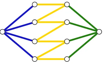
Figure 2.1: The underlying graphs of a pair of matroids (left) and the underlying graph

of the graphic matroidM1p1,p2M2 (right), whereM1, M2 is the pair of matroids shown

in the left part of the figure and p1, p2 are the edges represented by dashed lines.

settled in [69, 70] for general matroids (given by an oracle).

Theorem 18 (Corollary 7.2, [69]). For each k, there is an O(|E|4₎ _algorithm

constructing a decomposition of width at most 3k − 1 or concluding that the matroid has branch-width at least k+ 1.

Moreover, for matroids representable over a fixed finite field, an efficient

algo-rithm for constructing a branch decomposition of optimal width is given in [43].

Let M1 and M2 be two matroids satisfying pi ∈E(Mi), for i∈ {1,2}. Then,

the 2-sum M1p1,p2 M2 is defined as the matroid with the set of circuits below:

C =C(M1\p1)∪ C(M2 \p2) ∪

{(C1\p1)∪(C2\p2) :pi ∈Ci ∈ C(Mi) for i∈ {1,2}}.

An example of a 2-sum of a pair of graphic matroids can be found in Figure 2.1.

A monadic second-order (MSO) formula ψ for a matroid M can contain the following:

logical connectives∨,∧,¬,⇒,

(36)

quantifications∃xover elements ofE(M) – in this case, we callxan element variable,

quantifications∃X over subsets ofE(M) – there,X is calleda set variable,

the predicate x∈X of containment of an element in a set,

and, finally, the independence predicate ind(X) determining whether a

sub-setX of E(M) is independent.

In line with the above, lowercase letters (such asx1, x2, . . .) are used to denote

el-ement variables while uppercase letters (such asX1, X2, . . .) denote set variables.

Deciding MSO properties of matroids is NP-hard in general, since, for

exam-ple, the property that a graph is hamiltonian can be determined by deciding the

following formula on the graphic matroid corresponding to the input graph:

∃H∃e is circuit(H)∧is base(H\ {e}),

where H is a set variable, e an element variable, and is circuit(·) and is base(·) are predicates testing the property of being a circuit and a base, respectively.

These can be defined in MSO logic as follows:

is circuit(H)≡ ¬ind(H)∧ ∀e: (e ∈H)⇒ind(H\ {e}),

is base(H)≡ ¬ ∃e: ind(H∪ {e})

(37)

Chapter 3 Permutation Pattern Matching

In this chapter, we study an algorithmic problem where we are given two

permu-tationsσ andπ and are interested in whetherσ is a pattern ofπ. A permutation

π contains a permutation σ as a pattern if it contains a subsequence of length

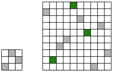
[image:37.595.225.412.465.583.2]

|σ| whose elements are in the same relative order as in the permutation σ. This is illustrated in Figure 3.1.

Figure 3.1: A representation of the permutation matrices of permutations (1,3,2)

and(9,2,4,5,10,8,6,1,7,3). White positions of the grid correspond to 0-entries of the

permutation matrix, non-white positions to 1-entries, the columns are indexed from left

to right, the rows from bottom to top. Thus, the (1,1)entry of both matrices is located

in the bottom-left corner. The former permutation is contained within the latter as a

pattern. One of the occurrences of the pattern is highlighted in green.

The properties of such a partial order on the set of all permutations have

been investigated from a variety of angles in discrete mathematics, particularly

(38)

in enumerative combinatorics. Knuth [55] has shown that the number of

permu-tations avoiding (2,3,1) is the nth _{Catalan number. Various choices of prohibited}

patterns have been studied among others by Lov´asz [60], Rotem [77], and Simion

and Schmid [80]. This culminated in the Stanley-Wilf conjecture stating that for

every fixed prohibited pattern, the number of permutations of length n avoiding it can be bounded by cn _{for some constant} _c_{. Klazar [54] reduced the question}

to the F¨uredi-Hajnal conjecture, which was ultimately proved by Marcus and

Tardos in 2004 [65].

Wilf [83] also asked the algorithmic question of whether detecting a given

pattern (of length `) in a given permutation (of length n) can be done in subex-ponential time. Subsequently, the problem was shown to be NP-hard in [12].

Ahal and Rabinovich have obtained an O(n0.47`+o(`)_{) time algorithm [1]. Fast}

algorithms have been found for certain restricted versions of the problem [12, 48].

The linear time dynamic programming algorithm for finding the longest

increas-ing subsequence [78] is even a standard content of many undergraduate courses

on algorithms.

Pattern matching has also received interest in the context of parameterized

complexity. Several groups of researchers have obtained W[1]-hardness results

for generalizations of the problem [15, 39]. For example, in one such

gener-alization the input permutations are colored and the requirement is to find a

color-preserving occurrence of the pattern. In [14] it was shown that the problem

is in FPT when parameterized by the number of runs (maximal monotonic

con-secutive subsequences) in the target permutation. The authors of [14] raise the

issue of whether their problem has a polynomial size kernel as an open problem.

(39)

has been resolved by Guillemot and Marx [39], who obtained an algorithm with

asymptotic running time of 2O(`2_log_`₎

·n. This implies the existence of a kernel for the problem. Obtaining kernel size lower bounds was posed as an open question

during a plenary talk at Permutation Patterns 2013 by St´ephane Vialette.

In what follows, we prove that the permutation pattern problem under the

standard parameterization by` does not have a polynomial size kernel (assuming

NP 6⊆co-NP/poly). This is achieved by introducing a novel polynomial reduction from the_Cliqueproblem to_{Permutation Pattern Matching}and applying

the cross-composition machinery described in Section 2.9.

3.1 Problem definition and additional notation

Definition 19. A permutation σ on the set [l] is a pattern of a permutation π

on the set [n] if there exists an increasing function ϕ: [l]→[n] such that

∀x, y ∈[l] :σ(x)< σ(y) if and only if π(ϕ(x))< π(ϕ(y)).

We say that the mapping ϕcertifies the pattern.

Permutation Pattern Matchingis the following parameterized

algorith-mic problem:

Input: a permutation σ on [`], a permutationπ on [n]. Parameter: `.

Question: isσ a pattern of π?

(40)

the target permutation.

In the sections below, we use the following additional notation. Recall there

are two common representations of a permutation πare used in the thesis: using the vector (π(1), π(2), . . . , π(n)) and using a permutation matrix. Both are illus-trated in Figure 3.1. A vector obtained from the vector representation by omitting

some entries is a subsequence of the permutation. Such subsequence is a

consec-utive subsequence if it contains precisely the entries with indexes from [i, j] for somei, j ∈N. We useπ[i, j] to denote the set of entries{π(i), π(i+ 1), . . . , π(j)}. A monotonic subsequence is a subsequence whose entries form a monotonic

se-quence. A run is a maximal monotonic consecutive subsequence. For example,

(4,5,3,1,2) contains a (decreasing) run of length 3.

3.2 Kernelization lower bounds

The main result of this thesis is the following theorem, which has already been

stated in Introduction.

Theorem 2. Unless NP ⊆ co-NP/poly, the Permutation Pattern Match-ing problem does not have a polynomial kernel.

We prove Theorem 2 using Theorem 17. However, this requires a polynomial

time reduction that allows cross-composition without significantly increasing the

parameter value. Reductions described in the literature [12, 15] have resisted our

attempts to apply the framework. Therefore, we introduce a new NP-hardness

proof that directly leads to a cross-composition. The new reduction is from the

well known Clique problem.

(41)

producing a permutation. The key property of the encoding is that for any

clique Kl on l vertices and any graphH we have Kl ⊆H if and only if πz(Kl) is

a pattern ofπz(H) for some particular choice of z. (The value of z depends only

on the size of the largest connected component of H.) This allows us to express the Clique problem in terms of Permutation Pattern Matching.

The definition of π(·) is somewhat technical although the basic idea is quite simple: we embed the upper-triangular submatrix of the adjacency matrix of the

input graph into a permutation. This is illustrated in Figure 3.2, where one can

see the permutation matrix of one such encoding permutation. In what follows,

we first give a rough sketch of how the construction of the encoding is organized.

Then, we describe the individual parts of the resulting permutation in more detail

and introduce some notation. Finally, the precise definition is given.

The encoding permutation itself consists of two types of entries: encoding

entries and separating entries. The former encode the edges of G. The encoding entries of the same vertex form a consecutive subsequence of the permutation.

The separating entries form decreasing runs used to separate encoding entries

of different vertices. Looking at πz(G) as an embedding of the upper-triangular

submatrix of the adjacency matrix ofGoffers another perspective: the separating runs mark where each row and column begins and ends, the encoding entries

determine where the 1-entries of the matrix are.

We start constructing πz(G) by imposing a total order onV(G) placing

(42)

assume that V(G) = [n] and set

N_G+(v) :={u:u > v∧ {u, v} ∈E(G)}, N_G−(v) :={u:u < v∧ {u, v} ∈E(G)},

deg+_G(v) :=|N_G+(v)|,

deg−_G(v) :=|N_G−(v)|.

The vertices from the sets N_G+(v) and N_G−(v) are calledthe right-neighbours and left-neighbours ofv, respectively. We now give a general overview of the structure of the permutation πz(G); the specification of the exact values and indexes

employed is postponed to the following paragraphs. The permutation starts

with a decreasing run of lengthz, continues with the entries encoding the vertex 1 (i.e., encoding N_G+(1)), which is then followed by another decreasing run of lengthz. This finishes the part of the permutation dedicated to the vertex 1 and the segment for the vertex 2 begins. Again, it starts with another decreasing run

of length z, continues with the encoding entries of N_G+(2), and is finished by a decreasing run of lengthz. This continues for all vertices ofG. Note that for each vertex v there is a pair of decreasing runs immediately surrounding the entries encoding N_G+(v), one from left and one from right. These are called the left and right separating runs of v, respectively. Together, we call these entries the pair of separating runs of v. For example, four pairs of separating runs are depicted in Figure 3.2.

To facilitate the formal definition ofπz(G), we begin by introducing a notation

for important positions and values of the resulting permutation’s entries. This

(43)

they start, or the positions where the parts encodingN_G+(v), for individual choices of v, start.

We use pL(v) and pR(v) as a shorthand for the positions on which the left

and right separating run of v starts, respectively. The first position of the seg-ment encoding N_G+(v) is denoted by pM(v). This is illustrated in Figure 3.2.

Specifically, we set pL(1) := 1, pM(1) := z + 1, and pR(1) := z + 1 + deg+G(1).

pL(1)

pM(1)

pR(1)

pL(2)

pM(2) · · ·

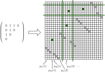
[image:43.595.138.500.253.505.2]

0 1 1 0 0 1 0 1 0 0            

Figure 3.2: Left part shows the upper triangular submatrix of the adjacency matrix

of a graph G = {1,2,3,4},

{1,2},{2,3},{2,4},{3,4} . The right part shows the permutation matrix representation of its encoding permutation π3(G). Once again,

the columns of both matrices are indexed from left to right, the rows from bottom to

top. White positions of the grid on the right correspond to 0-entries of the

permu-tation matrix, non-white positions are 1-entries. Separating runs are colored in light

gray, encoding entries in dark green. Note the one-to-one correspondence between the

1-entries of the matrix on the left with the encoding entries of the permutation matrix.

Horizontal green lines represent values attained at positions L(4) and R(4). Vertical

green lines denote indexes L(2) and R(2). Note that these four green lines induce a

rectangle with a single 1-entry. This encodes the 1-entry in the top-most position of the

second column of the adjacency matrix. Arrows below the permutation matrix illustrate

(44)

For v ≥2, we have:

pL(v) :=pR(v−1) +z,

pM(v) :=pL(v) +z,

pR(v) :=pM(v) + deg+G(v).

We also introduce notation for the values used by the separating runs. The left

separating run of v starts at the position pL(v) with the value qL(v). The right

separating run starts at pR(v) with the value qR(v). Finally, qM(v) is the least

value used by the encoding entries of vertices from N_G−(v) to determine their connection to v. (Specifically, vertices of N_G−(v) use the values [qM(v), qM(v) +

deg−_G(v)−1] to encode this. If deg_G−(v) is zero, the value qM(v) is actually not

used.) We setqL(1) := 2z, qM(1) :=z+ 1, and qR(1) :=z. For v ≥2, let

qR(v) :=qL(v−1) +z,

qM(v) :=qR(v) + 1,

qL(v) :=qM(v) +z+ deg−G(v)−1.

We now define the values of π=πz(G). For eachv, we introduce a decreasing

(45)

π(pL(v)) :=qL(v),

π(pL(v) + 1) :=qL(v)−1,

π(pL(v) + 2) :=qL(v)−2,

. . .

π(pL(v) +z−1) :=qL(v)−(z−1).

We also insert a decreasing run which starts at the position pR(v) with the value

qR(v):

π(pR(v)) :=qR(v),

π(pR(v) + 1) :=qR(v)−1,

π(pR(v) + 2) :=qR(v)−2,

. . .

π(pR(v) +z−1) :=qR(v)−(z−1).

This describes the entries represented by gray squares in Figure 3.2.

The remaining values are used to encode the edges of G. The neighbourhood

N_G+(v) is encoded by an increasing run on positionspM(v), pM(v)+1, . . . , pM(v)+ |N_G+(v)| − 1. We fix a vertex v ∈ V(G) and iterate through the neighbours

{u1, u2, . . . , uk}=NG+(v). Assume u1 < u2 < . . . < uk. For i∈[k], we set:

(46)

where `(v, ui) =|{w :w < v∧ {w, ui} ∈E(G)}|. The term `(v, ui) ensures that

no value in π is repeated.

The above procedure is carried out for each v ∈ V(G). This finishes the construction of πz(G). We now provide two observations.

Observation 20. For any graph Gand z ∈N the functionπz(G) is a

permuta-tion.

Proof. Let π :=πz(G). It is straightforward to verify that π is a mapping from

[p] to [p], for p = 2zn+|E(G)|. It remains to show that π is injective, i.e. that there is no pair of distinct indexes i, j such that π(i) = π(j). It can easily be seen that such i andj cannot both be an index of an entry forming a separating run, since the separating runs are explicitly constructed so that the sets of their

values are disjoint. For each vertex v there are exactly deg−_G(v) values between the values of its left and right separating run. These values are used to encode

the deg−_G(v) edges connecting v to its left-neighbours. The left-most neighbour is using the least value, the subsequent vertices are using values that increase by

1 with each neighbour (cf. the term `(v, ui) in equation (3.1)). Therefore, we

have neither a collision between a separating entry and an encoding entry nor

a collision between two entries encoding N_G−(v) for the same v. Finally, it can be easily seen that the sets of values encoding N_G−(v) are pairwise disjoint for different choices ofv.

Observation 21. For any choice of z ∈N and any choice of u, v ∈V(G), there is at most one 1-entry of πz(G) with an index in [pM(u), pR(u)−1] and value

in [qM(v), qM(v) + deg−G(v)−1]. Furthermore, there is an edge between vertices

(47)

Proof. The entries ofπ:=πz(G) with indexes from [pM(u), pR(u)−1] encode the

neighbourhood of the vertex u, i.e., N_G+(u). For each neighbour v from N_G+(u), we insert a single entry with value from [qM(v), qM(v) + deg−G(v)−1]. This is

because in equation (3.1) the term `(v, ui) is always strictly less than deg−G(v).

This implies both parts of the observation.

For the purpose of the proof of the lemma below, we define the following:

C(v) := [pM(v), pR(v)−1],

L(v) := pL(v) +bz₂c,

R(v) := pR(v) +bz₂c.

Therefore,C(v) is the set of entries of π encoding the vertex v,L(v) denotes the middle entry of the left separating run of v, and R(v) is the middle entry of the right separating run of v. Once more, Figure 3.2 illustrates the notation.

The following lemma implies NP-hardness of the studied problem:

Lemma 22. For every clique G, Kl is a subgraph of G if and only ifπz(Kl) is a

pattern of πz(G), for z = 4n0+ 4,where n0 is the number of vertices in the largest

connected component of G.

Proof. We let σ:=πz(Kl) and π :=πz(G).

IfGcontains a cliqueKlof sizel as a subgraph, thenπcontains the patternσ

by construction. This is because if we consider the permutation matrix

represen-tation ofπ and delete all columns except the ones that correspond to separating and encoding entries for vertices ofKl⊆G, we get a matrix that differs from the

(48)

the connection of the vertices of Kl to the vertices outside of Kl. By deleting

these columns (and the empty rows resulting from the above deletions) we arrive

at the permutation matrix representation of σ, implyingσ is a pattern ofπ. For the other direction, assume there is a function ϕ: [|σ|]→[|π|] certifying the pattern. We start by noting that there are no decreasing subsequences of

length 1₄z in π avoiding all separating runs. This is because such a sequence contains at most one entry from C(v) for each v ∈ V(G). At the same time, it cannot simultaneously contain an entry from C(u) and C(v) for u, v chosen from different connected components. This is because the construction of the

encoding permutation places vertices from the same component consecutively

and the entries encoding a component placed earlier in the ordering have strictly

smaller values than those from a later component. This bounds the length of the

subsequence by n0 < 1₄z.

Furthermore, any decreasing subsequence of π contains entries from at most one pair of separating runs. This is because once the sequence hits a separating

run of a vertexv, all its subsequent entries can only be from the pair of separating runs ofv. Any decreasing subsequence therefore starts with less than 1₄zencoding entries, which are then followed by entries of a pair of separating runs of some

vertex.

We now show that the certifying function ϕ naturally leads to a mapping from V(Kl) to V(G). Consider any vertex v ∈ V(Kl). The function ϕ maps

(49)

implies that the middle entryL(v) of the left separating run ofv inσneeds to be mapped by ϕto the left separating run ofu∈G. Additionally, the middle entry

R(v) of the right separating run ofv inσ needs to be mapped byϕsomewhere in the right separating run of the same vertex u. The above establishes a mapping from V(Kl) to V(G) denoted byfϕ.

We claim fϕ to be a graph homomorphism. Fix any pair of vertices v1, v2

of Kl such that v1 < v2. We show that fϕ(v1), fϕ(v2) are connected by an

edge in G. Since there is an edge between v1 and v2 in Kl, Observation 21

implies that the set of values σ[L(v1), R(v1)] contains precisely one number p

with σ(R(v2))≤ p≤ σ(L(v2)). Since ϕ certifies the pattern σ in π, there needs

to be an entry of π with an index between ϕ(L(v1)) and ϕ(R(v1)) and value

between π(ϕ(R(v2))) and π(ϕ(L(v2))). Observation 21 then implies there is an

edge between fϕ(v1) and fϕ(v2). Thus, fϕ is a homomorphism and Gcontains a

clique of size l.

The above reduction can be directly used within the cross-composition

frame-work to show our result.

Proof of Theorem 2. We set L to be the set of all pairs (Kl, G), where Kl is a

clique, G is a connected graph containingKl as a subgraph. It is widely known

that deciding x∈L is NP-complete.

We introduce a cross-composition ofLinto_{Permutation Pattern}

Match-ing. Let R be an equivalence relation on {0,1}∗ with the following properties:

the binary sequences that are not representing a pair (Kl, G), where Kl is a clique

(50)

respectively, is related in R if and only if|V(K1₎_|₌_|_V₍_K2₎_|_,_|_V₍_G1₎_|₌_|_V₍_G2₎_|_.

Clearly,R is a polynomial equivalence relation. For instances (Kl, G1), (Kl, G2),

(Kl, G3), . . ., (Kl, Gt) from the same equivalence class of R, we produce an

in-stance of the Permutation Pattern Matching problem where we ask if

πz(Kl) is in πz(G), where G is a disjoint union of graphsG1, . . . , Gt and z is set

to 4· |V(G1)|+ 4. Lemma 22 shows that the answer to this problem is YES if

and only if at least one of the instances (Kl, Gi) belongs to L. Since the

pa-rameter of the pattern matching instance is |πz(Kl)|, which can be bounded by |V(Gi)| ·2z+|V(Gi)|2 for any i, we can apply Theorem 17.

3.3 Conclusion

Guillemot and Marx [39] have shown that thePermutation Pattern

Match-ing problem can be solved in 2O(`2log`) ·n time. They raised the question of

whether a faster FPT algorithm could be obtained and outlined a strategy for

achieving this using their notion of decompositions of permutations. This relied

on the bound from the Stanley-Wilf conjecture not being tight. However, Fox [36]

has shown the bound is actually tight for almost all permutations. (Still, Fox [36]

gives an improved 2O(`2₎

·n algorithm.)

Note that in order to rule out kernels of size P(n) for any polynomial P(·), it suffices to find a cross-composition satisfying some polynomial constraint on

the value of the parameter of the resulting instance. In particular, the strength

of our bound does not depend on how slowly the value of the parameter of the

resulting instance grows. Our result rules out all polynomial upper bounds on

(51)

Chapter 4 Optimum Linear Arrangement

In the present chapter we give subexponential computational complexity lower

bounds for the_{Optimum Linear Arrangement} problem relative to the_Min

Bisection problem ond-regular graphs. This is achieved by introducing a

poly-nomial reduction from (a variant of) the Min Bisection problem to the

Op-timum Linear Arrangement problem. The key property of this reduction,

which allows us to prove our bounds, is that the instances of the former problem

result in instances of Optimum Linear Arrangement with at most O(nd)

edges. Therefore, the size of the instance is increased only linearly.

This reduction employs expanders in a black-box manner. We use the

al-gorithm implicit in Theorem 12 to construct these expanders. Other efficient

constructions could be substituted. Actually, any efficient construction

generat-ing d-regular graphs G with Cheeger number h(G) ≥ d

C for some fixed constant

C ∈ N would suffice – potentially at the cost of an increase in multiplicative constants irrelevant for the main hardness result. Let us note that this is one

of the aspects in which the contents of this chapter differ from the treatment in

the corresponding conference paper [6]. In this thesis, we assume the expander

Parameterized complexity : permutation patterns, graph arrangements, and matroid parameters

Permutation Patterns, Graph Arrangements,

and Matroid Parameters

by

Luk´

aˇs Mach

Thesis

Submitted in partial fulfilment of the requirements

for the degree of

Doctor of Philosophy

Contents

Acknowledgements

Declarations

Abstract

Chapter 1

Introduction

Chapter 2

Preliminaries

2.1

Basic notation

2.2

Permutations

2.3

Graphs

2.4

Algorithms

2.5

Complexity classes

2.6

Common hypotheses in complexity theory

2.7

Exponential Time Hypothesis

2.8

Expanders

2.9

Parameterized complexity and kernelization

2.10

Matroids

2.11

Width parameters for matroids

Chapter 3

Permutation Pattern Matching

3.1

Problem definition and additional notation

3.2

Kernelization lower bounds

3.3

Conclusion

Chapter 4

Optimum Linear Arrangement