International Journal of Engineering
J o u r n a l H o m e p a g e : w w w . i j e . i r
Real-time Scheduling of a Flexible Manufacturing System using a Two-phase
Machine Learning Algorithm
M. Namakshenas, R. Sahraeian*
Department of Industrial Engineering, College of Engineering, Shahed University, Tehran, Iran
P A P E R I N F O
Paper history:
Received 21 February 2013 Received in revised form 15 April 2013 Accepted 18 April 2013
Keywords:
Flexible Manufacturing Systems Real-time Scheduling Machine Learning Discrete-event Simulation Neural Network
A B S T R A C T
The static and analytic scheduling approach is very difficult to follow and is not always applicable in real-time. Most of the scheduling algorithms are designed to be established in offline environment. However, we are challenged with three characteristics in real cases: First, problem data of jobs are not known in advance. Second, most of the shop’s parameters tend to be stochastic. Third, thousands of jobs should be scheduled in a long planning horizon. In this work we designed an expert model for achieving better performance of real-time scheduling tasks in a flexible manufacturing system (FMS). The proposed expert model is comprised of two sets of modules, namely FMS simulator and decision (control) modules. Information is translated from the first set of modules to the second in two phases. First, a feed-forward neural network as a supervised machine learning mechanism is set to capture the queueing attributes of the shop and train in initialization and pre-run mode. Second, system states (in real run) are interpreted to the control module which is comprised of interconnected online learning activation function and a feed-forward neural net, and finally the best strategy is selected. Therefore, an interactive discrete-event simulation model with control module is implemented in order to evaluate different scenarios and reduce the computational time and complexity. Eventually, the presented procedure is benchmarked through simulation modeling of a triple-stage-triple-machine flexible flow shop with some embedded stochastic concept. Results support our proposed methodology and follow our overall argument.
doi: 10.5829/idosi.ije.2013.26.09c.13
1. INTRODUCTION1
In many flexible manufacturing systems (FMS), it is necessary to set up a set of competent techniques in the processing of jobs in order to keep up the pace of change in customer needs. Many of the systems used in our modern society ought to be such configured that they provide correct and on-time response to these changes. In case of schedulable real-time systems, the goal is to meet the deadline of every task by ensuring that each task can complete execution by its specified deadline. This deadline is adopted from environmental constraints imposed by the application of system in real-time [1]. Moreover, we are faced with three important attributes of the tasks scheduling in real-time: shortage of tasks information in advance, stochasticity of the shop’s parameters, and long-term planning horizon.
1*Corresponding Author Email: [email protected] (R.
Sahraeian)
However, many researchers unanimously have concluded that there exists no certain rule, say sequencing rule, which is universally better than others. The most famous and simple rules are: shortest processing time (SPT), longest processing time (LPT), earliest due date (EDD) and first in queue (FIQ). The popular rules like SPT fail at light load levels and generous due date allowances [2] and as the complexity of problem increases, simple rules and respectively statically utilization of these rules don’t perform well with respect to dedicated objective function. One acceptable solution is to dynamically alternating these rules upon receiving undesirable signals from system and according to the system’s conditions such as shop congestion [3]. Many researchers (See for example [4-6]) have suggested that dynamically alternating the sequencing policies can be highly effective.
acquisition of knowledge can be very useful for tasks scheduling in real time. In such cases, the scheduling parameters have to be tuned very quickly so that the system will be able to continue to produce optimum performance quickly corresponding to the system state changes [10].
In this study, we used a feed-forward neural network in the control module suggesting that parts of the information, acquired from initialization mode, remains unchanged and the rest are updated through an online transfer function in real-time simulation, which enables the system to learn efficiently in online mode in the context of discrete-event system.
2. RELATED WORKS: A COMPARATIVE STUDY
According to Maccarthy and Liu [7], three types of approaches can be used for FMS scheduling in real-time: (1) Heuristics, priority rules and simulation, (2) Mathematical programming and (3) Artificial intelligence (AI) techniques. In the literature, various methods can be recognized according to these three approaches. These methods include composite priority rules, decomposition methods [11, 12], single-pass and multi-pass methods [13, 14], real time dispatching and dynamic selection of priority rules [4, 8], adaptive scheduling [14], discrete-event (stochastic) simulation [4, 5, 15, 16], neighborhood search [9] and machine learning techniques [3, 11, 17].
It Substantial number of priority rules (simple and composite) has been reported in the literature. Performance of some rules is better than others in particular cases; however, yet no rule has become known that universally outperforms the others. For example, rules such as weighted shortest processing time (WSPT), earliest modified operation due-date (EMODD), combination of critical ratio and shortest processing time (CR+SPT) and processing time plus work in queue of its next operation (PT+WINQ) have been reported to produce better performance in response to due-date embedded objective functions or reversely, they fail in other measures [16]. An advantage in applying simple or composite priority rules directly underlies in ease of implementation. However, many researchers have used these rules in conjection with other dynamic methods.
One of the useful heuristics for scheduling tasks in a FMS, particularly in presence of uncertainty, is decomposition -partial sequencing- method. This technique consists of subdividing the original problem into equally sized and more manageable sub-problems which are optimized and then the best combination is taken as solution to the problem in hand [18]. Different forms of Decomposition methods exist in the literature:
time-based, job-based and machine-based (for more information see [11]). In this study, a time-based decomposition approach is deployed to generate training samples.
Supported by object-oriented programming, queueing structure and capability of analysis the stochastic procedures, discrete-event simulation modeling basically regarded as a last resort (if analytical methods fail) in the performance evaluation of a system. As an instance, Barrett and Barman [3] and Jeong and Kim [6] put forth a simulation model for scrutinizing the effects of candidate dispatching rules, Nakasuka and Yoshida [19] and Li and Lin [9] used simulation as a knowledge acquisition tool, Kuo, et al. [8] and Vinod and Sridharan [20] also took advantage of simulation for testing different production scenarios and strategies. Since optimization of the parameters of decision module in an online control system is time-consuming [19], an interactive discrete-event simulation model with control module is implemented in order to evaluate different scenarios and reduce the computational time and complexity.
There exist two basic techniques, namely reactive (dynamic) and robust approach, for dealing with uncertainties and stochastic nature of a shop in real-time according to the literature. Despite of time-based decomposition method in which the planning horizon are decomposed into equal or unequal periods, reactive approach by selecting priority rules may well be suited to the shop in real-time case. In contrast, it would be unfavorable to the manager to expect an undesirable event (triggering) and then react to it. Furthermore, one might establish the measuring of robustness [11]. According to this, the probabilities of particular event can be estimated and the system will react with respect to the probability of the corresponding event in advance. There are also other efficient techniques for dealing with complex circumstance in the literature, e.g. single-pass and multi-single-pass methods. Single-single-pass period technique combines single priority rule and schedule generation procedures to construct a particular algorithm. Lova and Tormos [10] suggest that this combination is central to constructing a feasible schedule. In contrast, one might deploy a multi-pass approach when there are multiple buffers between stages. This method is the mixture of randomly sampling method and multi-priority rules method in the steady-state planning horizon.
complement human knowledge of scheduling tasks or development of rule selection without human intervention [21], Machine learning is basically taken to fully reflect the real-time information of production scheduling based on knowledge gaining from system behavior. Three types of technique exist with respect to machine learning concept: cased-based reasoning, neural network and trigger-based learning. Priore, et al. [3] conducted a comparison between these algorithms and Mouelhi-Chibani and Pierreval [22] used the second class (a multi-layer perceptron) to select priority rules in a FMS. A drawback might be in adjusting networks total weights in online mode. Consequently, in this study, we used a neural network with a different topology in the control module suggesting that parts of information ,acquired from initialization mode, remains unchanged and the rest are updated through transfer function in the real-time simulation, which enables the system to learn efficiently in online mode.
The rest of this study is organized as follows: First, an overview of machine learning mechanism is given in section three. Next section formulates the problem by the neural network and discrete-event simulation configuration. In section (5), the propose model is validated and the results are analyzed. Finally, section (6) concludes section (5) through a summary and recommendation for future research.
3. OVERVIEW OF MACHINE LEARNING: NEURAL NETWORK APPROACH
System components tend to have specific connections together. However the connection may vary from a simple cause and effect to a dynamic full-ecological connection. It is also required that some system parameters be estimated through these connections.
To attain the aforementioned goals, in this study a novel framework of discrete-event simulation and neural network through iteratively learning characteristics of queues in a FMS is proposed. In real time simulation, a linear transfer function allows the inputs of offline network to be adapted and learned from changes in the system. This process requires substantial amount of experimental work of collecting practical data for training neural network, of an appropriate learning structure. It is a demanding task to develop a sustainable algorithm for any instance with a reasonable and acceptable solution in real time. In the first step of design, machine learning mechanism is the sheer amalgamated structure of human intuition and machine computational capability [23]. This will chronologically develop a procedure that can adapt itself to the new changes in the system conditions.
There are two types of learning methods. The employed procedure can be either “supervised” or
“unsupervised”. In supervised learning or machine learning mechanism, the learning mechanism takes only a set of input data and known responses to the inputs, and seeks to construct an estimator model that generates reasonable prediction to new data. Nevertheless, in unsupervised learning, the system learns of itself by adapting to the structural features in provided input patterns. Therefore, the framework of input and output learning vector should be such interconnected that taken training policy is able to reach maximum estimation accuracy. Therefore, if we reassess the machine learning idea with the FMS concept, it can be elicited that if a set of jobs in the ith queue experiencing the state S which contributed to performance measure P, then the system can learn from state S, if the state S improves the performance measure P.
A popular form of constructing a supervised learning mechanism can be established through a neural network. A neural network is comprised of a number of interconnected neurons. The synapse (connection) between neurons has weights, which depicts the strength level of these connections. The philosophy behind the vast utilization of neural networks is that incentivized by their non-parametric properties of any linear and non-linear functions and they are capable of fast-learning when appropriate parameters are chosen.
A number of machine learning methods have been studied with regard to their applicability to scheduling. These techniques shall be categorized into four major groups: The first mechanism is referred to as rote learning. In this mode, even though the system saves old decisions that gave good results, it has no means of generalizing them and user should be very careful in implementing them in a complex environment in which the chances of observing the same state is very low. This form of learning is only useful when the number of possible scheduling instances is limited [11, 17].
Case Based Reasoning (CBR) is another machine learning paradigm being considered for application to scheduling problems. CBR seeks to exploit experience gained from past similar cases. The larger scheduling problem requires the identification of salient features of past schedules, generalization, and a mechanism for determining which stored case best matches and is useful in the problem context. CBR can be applied to multi-objective scheduling problems as well [3, 20].
mechanisms are classifier systems. The classifier system learns rules which were found to perform better than the application of any of the single heuristics alone. A chromosome (or string) in such algorithm representing a list of rules (e.g., priority rules) that are to be used in the successive steps (or iterations) of an algorithmic framework designed to generate schedules for the problem at hand [11,22].
4. PROPOSED STRATEGY
4. 1. Problem Formulation The topology of proposed neural net model is illustrated in Figure 1. In the first step, the states of queues are preprocessed through a linear transfer function, which can make the online learning possible, and fed as inputs to the network. Furthermore, consideration of time component cannot be neglected. For example, if the steady state period in the time horizon of shop simulation is T, then it is required that period T is decomposed into equal units of T/n with n training sets for network configuration. In this study, it is supposed that system can uniformly experience stochastic changes during the steady state period. This procedure can also be applied for both deterministic and nondeterministic flexible flowshop scheduling where all jobs ought to undergo waiting in buffers sequentially. Two phases are prescribed in the presented network. The first phase includes a linear transfer function so that corresponding weights ought to be updated in the real run. The philosophy behind choosing a linear transfer function in the first step is that it is easy to be learned and second all essential parameters can be included directly without any sophistication. The second phase consists of a multi-layer perceptron network which should be trained in initialization mode. Therefore, its weights are static during the simulation run. By letting Sij state j
corresponding to queue i and PRi selected rule for queue
i , it is assumed that PRis are set as input vector by
randomly sampling in pre-run mode (offline input) and responses gaining from simulation run are set as target vector in that mode (offline target or online input). Once the network is trained offline, the triggering signal generated from real-time simulation run induces the network and by feeding the states of queues as an online attribute vector at specific moment the appropriate priority rule will be selected. Let M number of system state, H number of hidden layer neurons and N number of candidate priority rules, then, in order to mathematically illustrate the offline network and online transfer function, the two following expressions can be written:
(2) (1)
_ i = i { [
å
H h (å
M ¢j. jh)+ h]. hi¢}+ ih j
Estimated PR F F S w a w b (1)
(3)
1 2 1 2
1 1 1 2
( , ,..., , , ,..., , ) ...
j j j Nj j j Nj
j j j j Nj Nj
S F S S S
S S S
l l l d
l l l d
¢ = =
+ + + + (2)
where wjh is the strength level of connection between jth
element of S¢jand hth neuron of hidden layer, Fh(1) ,αh
,Fi(2) and βi are activation function and threshold
component associated with hth and ith neuron, respectively, w¢hithe weight symbolizing the connection
between hth neuron of hidden layer an corresponding ith neuron of priority rules vector and S¢j the output of
linear online transfer function. λij is the strength weight
corresponding to state Sij and δ the threshold value of
linear transfer function F(3).
Expression (1) should be minimized through backpropagation technique. To put it precisely, errors generated from objective function are backpropagated to the neurons of each layer by the negative gradients. In this study, in order to approach a fast training speed for both minimization of expression (1) in offline mode and updating the weights of expression (2) in online mode, a well-known levenberg-marquadrt algorithm is used. The philosophy behind utilization of this algorithm is its design characteristic owing to the fact that there is no need to compute the hessian matrix; consequently, it can compute the gradient quickly. (For more information about this technique, see [25])
4. 2.Model Development By acquiring the training sets from discrete-event simulation with replication and uniformly sampling the simulation results in the time horizon, the network is trained offline. The parameters of online transfer function are updated with respect to defined performance criteria. The neural network implemented in this study is three-layer feedforward consisting of one input layer, one hidden and one output layer. For the reason that there exist large number of training samples, number of neurons associated with hidden layer is chosen slightly larger, say 15, for keeping away underfitting problem. Also, overfitting problem is considered to avoid misleading results of training condition. A tangent hyperbolic transfer function is used in conjunction with initialization net.
Figure 1. Offline and online training framework of Neural Network
Figure 2. General overview of proposed strategy (in real-time
run)
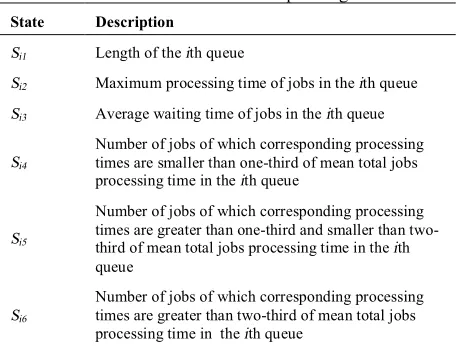
TABLE 1. Online attributes of queueing states
State Description
Si1 Length of the ith queue
Si2 Maximum processing time of jobs in the ith queue
Si3 Average waiting time of jobs in the ith queue
Si4
Number of jobs of which corresponding processing times are smaller than one-third of mean total jobs processing time in the ith queue
Si5
Number of jobs of which corresponding processing times are greater than one-third and smaller than two-third of mean total jobs processing time in the ith queue
Si6
Number of jobs of which corresponding processing times are greater than two-third of mean total jobs processing time in the ith queue
Before configuring the network, data collected from each state are normalized to have the same effect when processing through activation function. During the offline training, a set of equal-length intervals [#PR1#(t1,t2), #PR2#(t2,t3), … , #PRn#(tn,tn+1)] is used
for offline input and later in selection of priority rules in online mode. For example, if the network yields a constant a/3 and intervals are [#SPT#(0,a), #LPT#(a,2a)] ,we use SPT as selected priority rule. Performance criterion monitors FMS simulator for any disturbance, if an event degrades the performance, then a signal is sent to both triggering module and for online transfer function to updates its weights. Later, control module sends a best suited signal corresponding to priority rule module for rule selection. This procedure is outlined in Figure 2.
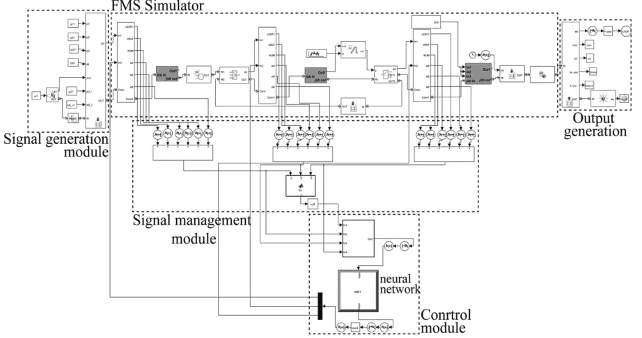
The simulation model is constructed in a modular way, of which each perform a particular role. There are three types of module deployed in this model: (1) Signal generation module, (2) Signal management module and (3) physical modules. The role of the first class of modules is generating signal for simulating breakdowns, reworks, etc. The second class interprets the signal in order to acquire desired signal like control module or triggering module and the third class are physical entities such as jobs.
Steps of the Algorithm:
1) Simulate and run the shop model.
2) Collect inputs and outputs for training offline network.
3) Set coefficients of online transfer function to be unit.
4) Re-run the simulated model which is connected to the
network (real time).
5) Upon receiving a signal implying that the previously
network alternates the existing rule and then updates the
online transfer function weights.
6) Repeat step 5 until running the simulation model stops.
5. EXPERIMENTAL STUDY
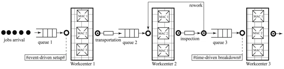
5. 1.The Proposed FMS Model The basic model is based on computer simulation study proposed by Barrett and Barman [24] and further employed in other pertinent articles (see for example [19, 22]). However, some stochasticity is embodied to measure the reliability of the proposed methodology. Thus, a specific hybrid flow shop model called ‘ triple-stations-triple-machines’ are put forth for study in the representation of a FMS in real-time. The presented model is comprised of three stations and each station has three machines which can do parallelly the same operations. Each job upon arrival to the work center goes to the first free machine. If all machines are loaded, the job waits in a queue until a machine becomes free. Transportation time from work center 1 to work center 2 assumes to be 0.3 units with a constant speed. Machines require 0.5 time units for changing tools periodically upon servicing 50 jobs, and it is supposed that absent machine operators can be replaced without disrupting production. Inspection time after jobs processing on work center 2 is negligible, however it assumes that 10% of the completed jobs requires rework; with rework time of 0.1 unit at work center 2 and also waiting jobs for rework have the highest priority among other jobs in queue. A time-based (independent of processed jobs) repair operation needed for machines breakdown in work center 3 on the supposition that occurrence of machines failure follows an exponential distribution with 1/50 of the mean and duration of the breakdown is uniformly distributed over the interval (10,100). This component is the only one amongst virtual and physical components, which imposes stochasticity on the system Furthermore, Arrival and processing times of each job in any work center are not deterministic, exponentially distributed with mean of 1.0 time units and preemption is not
allowed. Due to the randomly generation of arrival times, it is also assumed that arrival times of jobs are uncorrelated with each other and are known in advance. The proposed FMS model for study is illustrated in Figure 3.
In order to evaluate objective function, say mean tardiness, due date parameter should be imposed on jobs completion times. Thus, with the lack of adequate exogenous due dates from customer, it is considered that system generate its due dates itself, namely controllable due dates, by total work content (TWK) method [25]. According to this, the due-date of each job is equal to the sum of the job arrival time and due-date allowance factor – the amount of time that the job will spend in the system- multiplied by the total processing time. Then, due dates could be established as follows:
1
shop loading ( n i) ,
i
ep
b
=
µ ´
å
(3)where DDi is the due date of job I, Arithe arrival time
of job I, k the due-date allowance factor and pij the
processing time of job I on machine j.
It is also suggested that random generation of jobs arrival and processing times in each work center ought to be circumscribed and such manipulated that it can simulate the shop congestion condition [26]. Due to the stochastic nature of the model, obtaining the exact formula for shop load determination is somewhat difficult. Therefore, the relationship between arrival, processing time of jobs and loads to the work center can be written as following:
,
i i ij
j
DD =Ar +k
å
p (4)where β is the mean arrival rate of jobs, n the number of work centers, epi the mean expected processing time of
jobs at work center i. Accordingly, the above expression suggests that if the load of the shop is constant, then increasing the mean rate of jobs arrival will reduce the mean processing time of jobs, and vice versa. In this study, 91 percent (heavily load) for shop loading has been chosen.
5. 2. Validation, Evaluation and Analysis of the Results In order to justify the performance of proposed methodology, a simulation model of previously mentioned configuration with neural network is developed and conducted. In this study, for the sake of ease in analysis of responses, four basic priority rules are deployed: SPT, LPT, EDD and FIFO. For statistics generation, a run length of 30000 hour is selected. The entire procedure (from neural network configuration to real-time simulation of the shop model) is programmed and simulated by Matlab & Simulink software package.
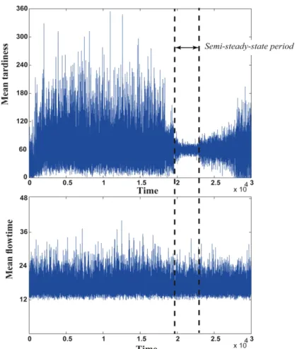
In this study, a multi-level verification [16] is implemented to ensure the correct configuration of simulated model and programming logic. For this purpose, five steps are performed: (1) Program debugging, (2) checking the consistency of internal logic, (3) plausibility checking through running model under different configuration of exogenous parameters (initial seeds), (4) steady state analysis and (5) schedulability test. A robust generalization of a simulated model substantially depends on steady state analysis. It is assumed that steady state period corresponding to run time h takes a fraction of h for which plotted moving average performance measure indicates a reasonably smaller variation. Due to the presence of randomnesses like breakdown, to some extent a pure steady phase could be elusive (semi-steady-state period). Figure 4 provides a summary plot of mean flowtime and mean tardiness moving average in the increments of simulation run length.
Figure 4. Steady state analysis of mean flowtime and mean
tardiness
Also, a schedulability test is employed to validate that a given task can satisfy its specified deadlines when scheduled according to a specific scheduling algorithm [1]. For example, in case of violent stochastic occurrence, even a best-known algorithm corresponding to a specific benchmark could yield a result which is far from predictions. Therefore, system is tested under different priority rules before reaching the steady state to ensure that tasks are schedulable.
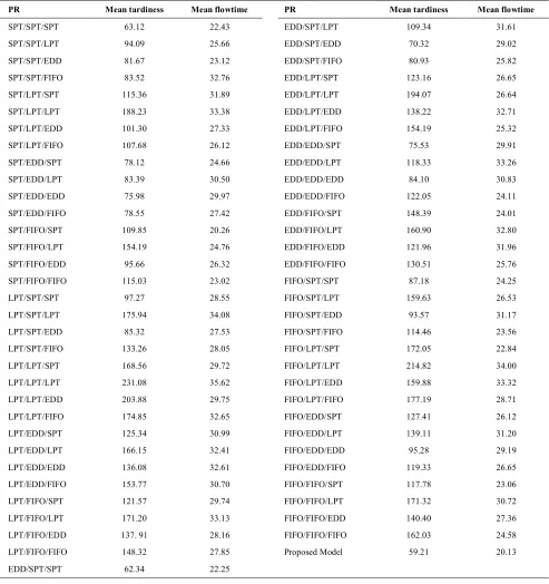
Table 2 summarizes the pertinent results of 64 combination of PR1/PR2/PR3 plus proposed strategy. For each combination 20 replications have been conducted. Note that PR1/PR2/PR3 represents the rules selected for respectively first, second and third queues. It is obvious that among all tested combinations EDD/SPT/SPT has shown better performance with respect to mean tardiness. Given the mean flowtime, SPT/FIFO/SPT gets the best score in comparison with other combinations. LPT/LPT/LPT exhibits the poorest result among other combinations in terms of both objective functions. The evidence suggests that (according to Table 2) the proposed strategy
outperforms EDD/SPT/SPT and SPT/FIFO/SPT
combinations in both measures. Figure 5 illustrates the overall density of priority rule selection in the planning horizon. It can be concluded that priority rules like LPT and FIFO are rarely chosen by control module, due to the degradation of performance criteria with respect to objective functions. Also, proposed simulation metamodel with control system are illustrated in Figure A.1.
Figure 5. Selected priority rules upon a triggering signal at
TABLE 2. Mean tardiness and mean flow time for priority rules and proposed strategy
PR Mean tardiness Mean flowtime PR Mean tardiness Mean flowtime
SPT/SPT/SPT 63.12 22.43 EDD/SPT/LPT 109.34 31.61
SPT/SPT/LPT 94.09 25.66 EDD/SPT/EDD 70.32 29.02
SPT/SPT/EDD 81.67 23.12 EDD/SPT/FIFO 80.93 25.82
SPT/SPT/FIFO 83.52 32.76 EDD/LPT/SPT 123.16 26.65
SPT/LPT/SPT 115.36 31.89 EDD/LPT/LPT 194.07 26.64
SPT/LPT/LPT 188.23 33.38 EDD/LPT/EDD 138.22 32.71
SPT/LPT/EDD 101.30 27.33 EDD/LPT/FIFO 154.19 25.32
SPT/LPT/FIFO 107.68 26.12 EDD/EDD/SPT 75.53 29.91
SPT/EDD/SPT 78.12 24.66 EDD/EDD/LPT 118.33 33.26
SPT/EDD/LPT 83.39 30.50 EDD/EDD/EDD 84.10 30.83
SPT/EDD/EDD 75.98 29.97 EDD/EDD/FIFO 122.05 24.11
SPT/EDD/FIFO 78.55 27.42 EDD/FIFO/SPT 148.39 24.01
SPT/FIFO/SPT 109.85 20.26 EDD/FIFO/LPT 160.90 32.80
SPT/FIFO/LPT 154.19 24.76 EDD/FIFO/EDD 121.96 31.96
SPT/FIFO/EDD 95.66 26.32 EDD/FIFO/FIFO 130.51 25.76
SPT/FIFO/FIFO 115.03 23.02 FIFO/SPT/SPT 87.18 24.25
LPT/SPT/SPT 97.27 28.55 FIFO/SPT/LPT 159.63 26.53
LPT/SPT/LPT 175.94 34.08 FIFO/SPT/EDD 93.57 31.17
LPT/SPT/EDD 85.32 27.53 FIFO/SPT/FIFO 114.46 23.56
LPT/SPT/FIFO 133.26 28.05 FIFO/LPT/SPT 172.05 22.84
LPT/LPT/SPT 168.56 29.72 FIFO/LPT/LPT 214.82 34.00
LPT/LPT/LPT 231.08 35.62 FIFO/LPT/EDD 159.88 33.32
LPT/LPT/EDD 203.88 29.75 FIFO/LPT/FIFO 177.19 28.71
LPT/LPT/FIFO 174.85 32.65 FIFO/EDD/SPT 127.41 26.12
LPT/EDD/SPT 125.34 30.99 FIFO/EDD/LPT 139.11 31.20
LPT/EDD/LPT 166.15 32.41 FIFO/EDD/EDD 95.28 29.19
LPT/EDD/EDD 136.08 32.61 FIFO/EDD/FIFO 119.33 26.65
LPT/EDD/FIFO 153.77 30.70 FIFO/FIFO/SPT 117.78 23.06
LPT/FIFO/SPT 121.57 29.74 FIFO/FIFO/LPT 171.32 30.72
LPT/FIFO/LPT 171.20 33.13 FIFO/FIFO/EDD 140.40 27.36
LPT/FIFO/EDD 137. 91 28.16 FIFO/FIFO/FIFO 162.03 24.58
LPT/FIFO/FIFO 148.32 27.85 Proposed Model 59.21 20.13
EDD/SPT/SPT 62.34 22.25
6. CONCLUSION
In this study, we presented a two-phase framework of a supervised machine learning approach. A discrete-event simulation in conjunction with proposed control module was implemented to study dynamic characteristics of a
initialization mode. Furthermore, there are two points in configuration of such expert model that we should refer to them:
1. Careful choice of system attributes should be taken into account. Developed model could be very sensitive or oblivious to considered states and yields misleading results.
2. There is no guarantee that that dynamically selection of priority rules will have better performance compared with static counterparts.
Though, we address the future work direction in the first step of design, defining more appropriate system architecture. We suggest that other machine learning architecture to be tested and developed in interaction with more complex FMS scheduling contexts, such as flexible job shop.
7. REFERENCES
1. Cheng, A. M., "Real-time systems: Scheduling, analysis, and verification", Wiley. com, (2003).
2. Park, Y., Kim, S. and Lee, Y.-H., "Scheduling jobs on parallel machines applying neural network and heuristic rules",
Computers & Industrial Engineering, Vol. 38, No. 1, (2000),
189-202.
3. Priore, P., de la Fuente, D., Puente, J. and Parreño, J., "A comparison of machine-learning algorithms for dynamic scheduling of flexible manufacturing systems", Engineering
Applications of Artificial Intelligence, Vol. 19, No. 3, (2006),
247-255.
4. Kuo, Y., Yang, T., Cho, C. and Tseng, Y.-C., "Using simulation and multi-criteria methods to provide robust solutions to dispatching problems in a flow shop with multiple processors",
Mathematics and Computers in Simulation, Vol. 78, No. 1,
(2008), 40-56.
5. Li, D.-C. and Lin, Y.-S., "Using virtual sample generation to build up management knowledge in the early manufacturing stages", European Journal of Operational Research, Vol. 175, No. 1, (2006), 413-434.
6. Tavakkoli-Moghaddam, R., Heydar, M. and Mousavi, S., "A hybrid genetic algorithm for a bi-objective scheduling problem in a flexible manufacturing cell", International Journal of
Engineering-Transactions A: Basics, Vol. 23, No. 3&4,
(2010), 235.
7. MacCarthy, B. and Liu, J., "Addressing the gap in scheduling research: A review of optimization and heuristic methods in production scheduling", The International Journal of
Production Research, Vol. 31, No. 1, (1993), 59-79.
8. Fakhrzad, M., Sadeghieh, A. and Emami, L., "A new multi-objective job shop scheduling with setup times using a hybrid genetic algorithm", International Journal of
Engineering-Transactions B: Applications, Vol. 26, No. 2, (2012), 207.
9. Tavakkoli-Moghaddam, R. and Mehdizadeh, E., "A new ilp model for identical parallel-machine scheduling with family setup times minimizing the total weighted flow time by a genetic algorithm", International Journal of Engineering Transactions
A: Basics, Vol. 20, No. 2, (2007), 183.
10. Nakasuka, S. and Yoshida, T., "Dynamic scheduling system utilizing machine learning as a knowledge acquisition tool", The
International Journal of Production Research, Vol. 30, No. 2,
(1992), 411-431.
11. Pinedo, M., "Scheduling: Theory, algorithms, and systems", Springer, (2012).
12. Choi, S. and Wang, K., "Flexible flow shop scheduling with stochastic processing times: A decomposition-based approach",
Computers & Industrial Engineering, Vol. 63, No. 2, (2012),
362-373.
13. Tormos, P. and Lova, A., "An efficient multi-pass heuristic for project scheduling with constrained resources", International
Journal of Production Research, Vol. 41, No. 5, (2003),
1071-1086.
14. Shiue, Y.-R. and Guh, R.-S., "Learning-based multi-pass adaptive scheduling for a dynamic manufacturing cell environment", Robotics and Computer-Integrated
Manufacturing, Vol. 22, No. 3, (2006), 203-216.
15. Song, L., Wang, P. and AbouRizk, S., "A virtual shop modeling system for industrial fabrication shops", Simulation Modelling
Practice and Theory, Vol. 14, No. 5, (2006), 649-662.
16. Vinod, V. and Sridharan, R., "Simulation modeling and analysis of due-date assignment methods and scheduling decision rules in a dynamic job shop production system", International Journal
of Production Economics, Vol. 129, No. 1, (2011), 127-146.
17. Kadaba, N., Nygard, K. E. and Juell, P. L., "Integration of adaptive machine learning and knowledge-based systems for routing and scheduling applications", Expert Systems with
Applications, Vol. 2, No. 1, (1991), 15-27.
18. Gupta, J. and Maykut, A., "Flow-shop scheduling by heuristic decomposition", International Journal of Production
Research, Vol. 11, No. 2, (1973), 105-111.
19. Mouelhi-Chibani, W. and Pierreval, H., "Training a neural network to select dispatching rules in real time", Computers &
Industrial Engineering, Vol. 58, No. 2, (2010), 249-256.
20. Jeong, K.-C. and Kim, Y.-D., "A real-time scheduling mechanism for a flexible manufacturing system: Using simulation and dispatching rules", International Journal of
Production Research, Vol. 36, No. 9, (1998), 2609-2626.
21. Michie, D., Spiegelhalter, D. J. and Taylor, C. C., "Machine learning, neural and statistical classification", Vol., No., (1994). 22. Pierreval, H., "Neural network to select dynamic scheduling
heuristics", Journal of Decision Systems, Vol. 2, No. 2, (1993), 173-190.
23. Mitchell, T. M. and Michell, T., Machine learning, 1997, McGraw-Hill Higher Education, New York, NY, USA. 24. Barrett, R. T. and Barman, S., "A slam ii simulation study of a
simplified flow shop", Simulation, Vol. 47, No. 5, (1986), 181-189.
25. Baker, K. R. and Trietsch, D., "Principles of sequencing and scheduling", Wiley. com, (2009).
26. Yang, S. and Wang, D., "A new adaptive neural network and heuristics hybrid approach for job-shop scheduling", Computers
APPENDIX:
Figure A.1. Simulation model with control module in Simulink
Real-time Scheduling of a Flexible Manufacturing System using a Two-phase
Machine Learning Algorithm
M. Namakshenas, R. Sahraeian
Department of Industrial Engineering, College of Engineering, Shahed University, Tehran, Iran
P A P E R I N F O
Paper history:
Received 21 February 2013 Received in revised form 15 April 2013 Accepted 18 April 2013
Keywords:
Flexible Manufacturing Systems Real-time Scheduling Machine Learning Discrete-event Simulation Neural Network هﺪﯿﮑﭼ
اﺮﺟاتﺎﯿﻠﻤﻋﯽﻟاﻮﺗيرﻮﺌﺗﺚﺣﺎﺒﻣرددﻮﺟﻮﻣﯽﻠﯿﻠﺤﺗيﺎﻫدﺮﮑﯾور،ﯽﻌﻗاوﻂﯾاﺮﺷرد ﺖﺴﯿﻧﯽﻧﺪﺷ
. ﻢﺘﯾرﻮﮕﻟازايرﺎﯿﺴﺑ يﺎﻫ
ﻂﯿﺤﻣرداردﻮﺧﯽﯾارﺎﮐدﻮﺟﻮﻣ ﯽﻣﺖﺳدزاﺎﯾﻮﭘيﺎﻫ
ﺪﻨﻫد . ﯽﻠﻋ ﻪﺼﺧﺎﺷﻪﺳ،ﻞﮑﺸﻣﻦﯾاﻢﻏر ﺶﻟﺎﭼ،ﯽﻌﻗاوﻂﯾاﺮﺷردﯽﻠﺻاي
ﺰﯿﮕﻧاﺮﺑ ﺖﺳا : ًﻻوا هداد، ﻪﻣﺎﻧﺮﺑياﺪﺘﺑاردﺎﻫرﺎﮐيﺎﻫ ﻧسﺮﺘﺳدرديﺰﯾر
ﺖﺴﯿ ًﺎﯿﻧﺎﺛ؛ هﺎﮔرﺎﮐﯽﻟﺮﺘﻨﮐيﺎﻫﺮﺘﻣارﺎﭘ، ،
ﯽﻟﺎﻤﺘﺣا ﺖﺳا ًﺎﺜﻟﺎﺛ؛ ،
ﻪﻣﺎﻧﺮﺑﻖﻓاﮏﯾرد نﺎﻣزﯽﺘﺴﯾﺎﺑرﺎﮐناراﺰﻫ،يﺰﯾر
ﺪﻧﻮﺷيﺪﻨﺑ . ﺳرﺮﺑﻦﯾارد هﺮﺒﺧﻢﺘﺴﯿﺳ،ﯽ ﻒﻄﻌﻨﻣيﺪﯿﻟﻮﺗﻢﺘﺴﯿﺳﻂﯿﺤﻣرديا
هﺪﺷﯽﺣاﺮﻃ ﺖﺳا
نﺎﻣزارﺎﮐيدﺮﮑﻠﻤﻋﺎﺑﺎﺗ ﺪﻫدمﺎﺠﻧاﯽﻌﻗاوﻂﯾاﺮﺷردارﺎﻫرﺎﮐيﺪﻨﺑ
. زاﻪﻋﻮﻤﺠﻣودﻞﻣﺎﺷهﺮﺒﺧلﺪﻣﻦﯾا
لوژﺎﻣ ) نﺎﻣدﻮﭘ ( ﯽﻠﮐيﺎﻫ ﺖﺳا : ﻪﯿﺒﺷ ﻢﯿﻤﺼﺗوهﺎﮔرﺎﮐزﺎﺳ هﺪﻧﺮﯿﮔ
) ﺮﻟﺮﺘﻨﮐ .( هداد ﻪﻋﻮﻤﺠﻣزاتﺎﻋﻼﻃاوﺎﻫ لواي
ﻪﻋﻮﻤﺠﻣﻪﺑ ي
ﯽﻣﺮﯿﺴﻔﺗزﺎﻓودردمود ﺪﻧﻮﺷ
. ﻪﮑﺒﺷﮏﯾاﺪﺘﺑا
ﺲﭘﯽﺒﺼﻋي
ﺑﺪﻧارﻮﺧ ﻪ ﯽﺗرﺎﻈﻧﯽﻨﯿﺷﺎﻣيﺮﯿﮔدﺎﯾمﺰﯿﻧﺎﮑﻣناﻮﻨﻋ ،
ﻪﺼﺧﺎﺷ يﺎﻫ
نزوﻪﺑلﺪﻣياﺮﺟازاﻞﺒﻗوﻪﺘﻓﺮﮔهﺎﮔرﺎﮐزاارﻢﺘﺴﯿﺳﻒﺻ ﯽﻣﻪﯿﻟواﯽﻫدراﺪﻘﻣدﻮﺧيﺎﻫﺮﺘﻣارﺎﭘوﺎﻫ
ﺪﻨﮐ .
تﻻﺎﺣ،ﺲﭙﺳ
ﻢﺘﺴﯿﺳ ) ﯽﻠﺻاياﺮﺟارد (
ﺟﻪﺑ ﺰ ء لﺎﻌﻓﻊﺑﺎﺗﻞﻣﺎﺷدﻮﺧﻪﮐﯽﻟﺮﺘﻨﮐ نآيزﺎﺳ
ﻪﮑﺒﺷوﻦﯾﻻ ﯽﺒﺼﻋي ﺖﺳا ﻦﯾﺮﺘﻬﺑوهﺪﺷﻪﻤﺟﺮﺗ،
ﯽﻣبﺎﺨﺘﻧايﮋﺗاﺮﺘﺳا دﻮﺷ
. ،ﻦﯿﻨﭽﻤﻫ رﻮﻈﻨﻣ ﻪﺑ مﻮﻬﻔﻣﺮﺑﯽﻨﺒﻣﯽﻟﺪﻣ،ﯽﺗﺎﺒﺳﺎﺤﻣنﺎﻣزﺶﻫﺎﮐوﻒﻠﺘﺨﻣيﺎﻫﻮﯾرﺎﻨﺳﯽﺑﺎﯾزرا
ﻪﯿﺒﺷ ﻪﺘﺴﺴﮔيزﺎﺳ
-ﺰﺟﺎﺑﻞﻣﺎﻌﺗردﺪﻣﺎﺸﯿﭘ ء
ﺑﯽﻟﺮﺘﻨﮐ ﻪ ﺖﺳاهﺪﺷﻪﺘﻓﺮﮔرﺎﮐ .
ﺗﺮﺜﮐاﺪﺣﻦﯿﮕﻧﺎﯿﻣفﺪﻫﻊﺑﺎﺗود ﺄ
وﺎﻫرﺎﮐﺮﯿﺧ
هﺪﺷﻪﺘﻓﺮﮔﺮﻈﻧردﯽﻟﺎﻤﺘﺣايﺎﻫﺮﺘﻣارﺎﭘﺎﺑﯽﻫﺎﮕﺘﺴﯾاﻪﺳفوﺮﻌﻣلﺎﺜﻣﯽﺑﺎﯾزراردﻢﺘﺴﯿﺳردﺎﻫرﺎﮐنﺎﯾﺮﺟنﺎﻣزتﺪﻣﻦﯿﮕﻧﺎﯿﻣ ﺖﺳا . هﺪﻨﻫدنﺎﺸﻧﺪﻫاﻮﺷوﺞﯾﺎﺘﻧ لﺪﻣﯽﯾارﺎﮐوهﺪﺷحﺮﻄﻣيﺎﻋدايرﺎﮔزﺎﺳي
ﺖﺳا .