Consistent Selection of Tuning Parameters
via Variable Selection Stability
Wei Sun [email protected]
Department of Statistics Purdue University
West Lafayette, IN 47907, USA
Junhui Wang [email protected]
Department of Mathematics, Statistics, and Computer Science University of Illinois at Chicago
Chicago, IL 60607, USA
Yixin Fang [email protected]
Departments of Population Health and Environmental Medicine New York University
New York, NY 10016, USA
Editor:Xiaotong Shen
Abstract
Penalized regression models are popularly used in high-dimensional data analysis to conduct vari-able selection and model fitting simultaneously. Whereas success has been widely reported in litera-ture, their performances largely depend on the tuning parameters that balance the trade-off between model fitting and model sparsity. Existing tuning criteria mainly follow the route of minimizing the estimated prediction error or maximizing the posterior model probability, such as cross vali-dation, AIC and BIC. This article introduces a general tuning parameter selection criterion based on variable selection stability. The key idea is to select the tuning parameters so that the resultant penalized regression model is stable in variable selection. The asymptotic selection consistency is established for both fixed and diverging dimensions. Its effectiveness is also demonstrated in a variety of simulated examples as well as an application to the prostate cancer data.
Keywords: kappa coefficient, penalized regression, selection consistency, stability, tuning
1. Introduction
Among other variable selection methods, penalized regression models have been popularly used, which penalize the model fitting with various regularization terms to encourage model sparsity, such as the lasso regression (Tibshirani, 1996), the smoothly clipped absolute deviation (SCAD, Fan and Li, 2001), the adaptive lasso (Zou, 2006), and the truncatedl1-norm regression (Shen et al., 2012). In the penalized regression models, tuning parameters are often employed to balance the trade-off between model fitting and model sparsity, which largely affects the numerical performance and the asymptotic behavior of the penalized regression models. For example, Zhao and Yu (2006) showed that, under the irrepresentable condition, the lasso regression is selection consistent when the tuning parameter converges to 0 at a rate slower thanO(n−1/2). Analogous results on the choice of tuning parameters have also been established for the SCAD, the adaptive lasso, and the truncatedl1-norm regression. Therefore, it is of crucial importance to select the appropriate tuning parameters so that the performance of the penalized regression models can be optimized.
In literature, many classical selection criteria have been applied to the penalized regression models, including cross validation (Stone, 1974), generalized cross validation (Craven and Wahba, 1979), Mallows’Cp(Mallows, 1973), AIC (Akaike, 1974) and BIC (Schwarz, 1978). Under certain regularity conditions, Wang et al. (2007) and Wang et al. (2009) established the selection consis-tency of BIC for the SCAD, and Zhang et al. (2010) showed the selection consisconsis-tency of generalized information criterion (GIC) for the SCAD. Most of these criteria follow the route of minimizing the estimated prediction error or maximizing the posterior model probability. To the best of our knowl-edge, few criteria has been developed directly focusing on the selection of the informative variables.
This article proposes a tuning parameter selection criterion based on variable selection stability. The key idea is that if multiple samples are available from the same distribution, a good variable selection method should yield similar sets of informative variables that do not vary much from one sample to another. The similarity between two informative variable sets is measured by Cohen’s kappa coefficient (Cohen, 1960), which adjusts the actual variable selection agreement relative to the possible agreement by chance. Similar stability measures have been studied in the context of cluster analysis (Ben-Hur et al., 2002; Wang, 2010) and variable selection (Meinshausen and B¨uhlmann, 2010). Whereas the stability selection method (Meinshausen and B¨uhlmann, 2010) also follows the idea of variable selection stability, it mainly focuses on selecting the informative vari-ables as opposed to selecting the tuning parameters for any given variable selection methods. The effectiveness of the proposed selection criterion is demonstrated in a variety of simulated examples and a real application. More importantly, its asymptotic selection consistency is established, show-ing that the variable selection method with the selected tunshow-ing parameter would recover the truly informative variable set with probability tending to one.
2. Penalized Least Squares Regression
Given that(x1,y1), . . . ,(xn,yn)are independent and identically distributed from some unknown joint distribution, we consider the linear regression model
y=Xβ+ε= p
∑
j=1
βjx(j)+ε,
where β = (β1,···,βp)T, y = (y1,···,yn)T, X = (x1,···,xn)T = (x(1),···,x(p)) with xi = (xi1,···,xip)T orx(j)= (x1j,···,xn j)T, andε|X∼N(0,σ2In). When p is large, it is also assumed that only a small number ofβj’s are nonzero, corresponding to the truly informative variables. In addition, bothyandx(j)’s are centered, so the intercept can be omitted in the regression model.
The general framework of the penalized regression models can be formulated as
argmin
β
1
nky−Xβk
2+ p
∑
j=1
pλ(|βj|), (1)
wherek · kis the Euclidean norm, and pλ(|βj|)is a regularization term encouraging sparsity inβ. Widely used regularization terms include the lasso penaltypλ(θ) =λθ(Tibshirani, 1996), the SCAD
penalty withp′λ(θ) =λ(I(θ≤λ) +(γλ−θ)+
(γ−1)λI(θ>λ))(Fan and Li, 2001), the adaptive lasso penalty pλ(θ) =λjθ=λθ/|βˆj| (Zou, 2006) with ˆβj being some initial estimate of βj, and the truncated
l1-norm penalty pλ(θ) =λmin(1,θ)(Shen et al., 2012).
With appropriately chosenλn, all the aforementioned regularization terms have been shown to be selection consistent. Here a penalty term is said to be selection consistent if the probability that the fitted regression model includes only the truly informative variables is tending to one, and λ is replaced by λn to emphasize its dependence onn in quantifying the asymptotic behaviors. In particular, Zhao and Yu (2006) showed that the lasso regression is selection consistent under the
irrepresentable condition when√nλn→∞andλn→0; Fan and Li (2001) showed that the SCAD
is selection consistent when√nλn→∞andλn→0; Zou (2006) showed that the adaptive lasso is selection consistent whennλn→∞and√nλn→0; and Shen et al. (2012) showed that the truncated
l1-norm penalty is also selection consistent whenλnsatisfies a relatively more complex constraint. Although the asymptotic order ofλnis known to assure the selection consistency of the penal-ized regression models, it remains unclear how to appropriately selectλnin finite sample so that the resultant model in (1) with the selectedλncan achieve superior numerical performance and attain asymptotic selection consistency. Therefore, it is in demand to devise a tuning parameter selection criterion that can be employed by the penalized regression models so that their variable selection performance can be optimized.
3. Tuning via Variable Selection Stability
3.1 Variable Selection Stability
For simplicity, we denote the training sample aszn. A base variable selection methodΨ(zn;λ)with a given training samplezn and a tuning parameterλyields a set of selected informative variables
A
⊂ {1,···,p}, called the active set. WhenΨis applied to various training samples, different active sets can be produced. Supposed that two active setsA
1andA
2are produced, the agreement betweenA
1andA
2can be measured by Cohen’s kappa coefficient (Cohen, 1960),κ(
A
1,A
2) =Pr(a)−Pr(e)1−Pr(e) . (2)
Here the relative observed agreement between
A
1andA
2isPr(a) = (n11+n22)/p, and the hypothet-ical probability of chance agreementPr(e) = (n11+n12)(n11+n21)/p2+ (n12+n22)(n21+n22)/p2, withn11=|A
1∩A
2|,n12=|A
1∩A
2c|,n21=|A
1c∩A
2|,n22=|A
1c∩A
2c|, and| · |being the set cardi-nality. Note that−1≤κ(A
1,A
2)≤1, whereκ(A
1,A
2) =1 whenA
1andA
2are in complete agree-ment withn12=n21=0, andκ(A
1,A
2) =−1 whenA
1 andA
2are in complete disagreement withn11=n22=0 andn12=n21=p/2. For degenerate cases with
A
1=A
2=/0orA
1=A
2={1, . . . ,p}, we setκ(/0,/0) =κ({1, . . . ,p},{1, . . . ,p}) =−1 under the assumption that the true model is sparse and containing at least one informative variable. As a consequence, the kappa coefficient in (2) is not suitable for evaluating the null model with no informative variable and the complete model with all variables. Based on (2), the variable selection stability is defined as follows.Definition 1 The variable selection stability ofΨ(·;λ)is defined as s(Ψ,λ,n) =Eκ(Ψ(Z1n;λ),Ψ(Zn2;λ)),
where the expectation is taken with respect to Zn1 and Z2n, two independent and identically training samples of size n, andΨ(Z1n;λ)andΨ(Z2n;λ)are two active sets obtained by applyingΨ(·;λ)to Z1n and Z2n, respectively.
By definition,−1≤s(Ψ,λ,n)≤1, and large value ofs(Ψ,λ,n)indicates a stable variable se-lection method Ψ(·;λ). Note that the definition of s(Ψ,λ,n) relies on the unknown population distribution, therefore it needs to be estimated based on the only available training sample in prac-tice.
3.2 Kappa Selection Criterion
Algorithm 1 (kappa selection criterion) :
Step 1. Randomly partition (x1,···,xn)T into two subsets z∗1b = (x1∗b,···,x∗mb)T and z∗2b = (x∗b
m+1,···,x∗2bm)T.
Step 2. Obtain
A
b∗b1λand
A
b2∗λbfromΨ(z1∗b,λ)andΨ(z∗2b,λ)respectively, and estimate the variable selection stability ofΨ(·;λ)in theb-th splitting byˆ
s∗b(Ψ,λ,m) =κ(
A
b∗b 1λ,A
b2∗λb).Step 3. Repeat Steps 1-2 for B times. The average estimated variable selection stability of Ψ(·;λ)is then
ˆ
s(Ψ,λ,m) =B−1
B
∑
b=1 ˆ
s∗b(Ψ,λ,m).
Step 4. Compute ˆs(Ψ,λ,m)for a sequence ofλ’s, and select
ˆ λ=min
n
λ: sˆ(Ψ,λ,m)
maxλ′sˆ(Ψ,λ′,m) ≥1−αn
o
.
Note that the treatment in Step 4 is necessary since some informative variables may have rela-tively weak effect compared with others. A large value ofλmay produce an active set that consis-tently overlooks the weakly informative variables, which leads to an underfitted model with large variable selection stability. To assure the asymptotic selection consistency, the thresholding value αn in Step 4 needs to be small and converges to 0 asn grows. Settingαn=0.1 in the numerical experiments yields satisfactory performance based on our limited experience. Furthermore, the sen-sitivity study in Section 5.1 suggests thatαnhas very little effect on the selection performance when it varies in a certain range. In Steps 1-3, the estimation scheme based on cross-validation can be replaced by other data re-sampling strategies such as bootstrap or random weighting, which do not reduce the sample size in estimating
A
b∗b1λand
A
b2∗λb, but the independence betweenA
b1∗λbandA
b2∗λbwillno longer hold.
The proposed kappa selection criterion shares the similar idea of variable selection stability with the stability selection method (Meinshausen and B¨uhlmann, 2010), but they differ in a number of ways. First, the stability selection method is a competitive variable selection method, which com-bines the randomized lasso regression and the bootstrap, and achieves superior variable selection performance. However, the kappa selection criterion can be regarded as a model selection criterion that is designed to select appropriate tuning parameters for any variable selection method. Second, despite of its robustness, the stability selection method still requires a number of tuning parameters. The authors proposed to select the tuning parameters via controlling the expected number of falsely selected variables. However, this criterion is less applicable in practice since the expected number of falsely selected variables can only be upper bounded by an expression involving various unknown quantities. On the contrary, the kappa selection criterion can be directly applied to select the tuning parameters for the stability selection method.
4. Asymptotic Selection Consistency
as
A
cT={p0+1,···,p}. Furthermore, we denotern≺snifrnconverges to 0 at a faster rate thansn,
rn∼snifrnconverges to 0 at the same rate assn, andrnsnifrnconverges to 0 at a rate not slower thansn.
4.1 Consistency with Fixed p
To establish the asymptotic selection consistency with fixedp, the following technical assumptions are made.
Assumption 1: There exist positivern andsn such that the base variable selection method is selection consistent if rn ≺λn≺sn. Let λn∗ be such a tuning parameter with rn ≺λ∗n≺sn, then
P(
A
bλ∗n =
A
T)≥1−εn for some εn→ 0. In addition, for any positive constant λ0, there exists positivec0(λ0)such that, whennis sufficiently large,P
\
λ0rn≤λn≤λ∗
n
{
A
bλn=
A
T}
≥1−c0(λ0), (3)
wherec0(λ0)converges to 0 asλ0→∞.
Assumption 1 specifies an asymptotic working interval forλn within which the base variable selection method is selection consistent. Here the consistent rateεnis defined forλ∗nonly, and needs not hold uniformly over allλn with rn≺λn≺sn. Furthermore, (3) establishes an uniform lower bound for the probability of selecting the true model whenλnis within the interval(λ0rn,λ∗n).
Assumption 2: Givenrnin Assumption 1, for any positive constantλ0, there existζn,c1(λ0)and
c2(λ0)such that, whennis sufficiently large, min
j∈ATP
\
rn−1λn≤λ0
{j∈
A
bλn}
≥1−ζn, (4)
min j∈Ac T
P
\
rn−1λn≤λ0
{j∈
A
bλn}
≥c1(λ0), (5)
max j∈Ac T
P
\
rn−1λn≥λ0
{j∈/
A
bλn}
≥c2(λ0), (6)
whereζn→0 asn→∞,c1(λ0)andc2(λ0)are positive and only depend onλ0, andc1(λ0)→1 as λ0→0.
Assumption 2 implies that ifλnconverges to 0 faster thanrn, the base variable selection method will select all the variables asymptotically, and whenλnconverges to 0 at the same rate ofrn, the base variable selection method will select any noise variable with an asymptotically positive probability. The inequalities (4)-(6) also establish uniform lower bounds for various probabilities of selecting informative variables or noise variables.
Assumptions 1 and 2 are mild in that they are satisfied by many popular variable selection methods. For instance, Lemma 2 in the online supplementary material shows that Assumptions 1 and 2 are satisfied by the lasso regression, the adaptive lasso, and the SCAD. The assumptions can also be verified for other methods such as the elastic-net (Zou and Hastie, 2005), the adaptive elastic net (Zou and Zhang, 2009), the group lasso (Yuan and Lin, 2006), and the adaptive group lasso (Wang and Leng, 2008).
Theorem 1 Under Assumptions 1 and 2, any variable selection method in (1) withλˆn selected as
in Algorithm 1 withαn≻εnis selection consistent. That is,
lim
n→∞Blim→∞P(b
A
ˆλn =
A
T) =1.Theorem 1 claims the asymptotic selection consistency of the proposed kappa selection criterion when p is fixed. That is, with probability tending to one, the selected active set by the resultant variable selection method with tuning parameter ˆλn contains only the truly informative variables. As long asαnconverges to 0 not too fast, the kappa selection criterion is guaranteed to be consistent. Therefore, the value ofαnis expected to have little effect on the performance of the kappa selection criterion, which agrees with the sensitivity study in Section 5.1.
4.2 Consistency with Divergingpn
In high-dimensional data analysis, it is of interest to study the asymptotic behavior of the proposed kappa selection criterion with divergingpn, where size of truly informative setp0nmay also diverge with n. To accommodate the diverging pn scenario, the technical assumptions are modified as follows.
Assumption 1a: There exist positivern andsn such that the base variable selection method is selection consistent if rn ≺λn≺sn. Let λn∗ be such a tuning parameter with rn ≺λ∗n≺sn, then
P(
A
bλ∗n =
A
T)≥1−εn for some εn→ 0. In addition, for any positive constant λ0, there exists positivec0n(λ0)such that, whennis sufficiently large,P \
λ0rn≤λn≤λ∗
n
{
A
bλn=
A
T}
≥1−c0n(λ0), (7)
where limλ0→∞limn→∞c0n(λ0)→0.
Assumption 2a: Givenrnin Assumption 1a, for any positive constantλ0, there existζn,c1n(λ0) andc2n(λ0)such that, whennis sufficiently large,
min j∈ATP
\
rn−1λn≤λ0
{j∈
A
bλn}
≥1−ζn, (8)
min j∈Ac T
P \
rn−1λn≤λ0
{j∈
A
bλn}
≥c1n(λ0), (9)
max j∈Ac T
P
\
rn−1λn≥λ0
{j∈/
A
bλn}
≥c2n(λ0), (10)
whereζnsatisfies pnζn→0 asn→∞,c1n(λ0)andc2n(λ0)are positive and may depend onnand λ0, and limλ0→0limn→∞c1n(λ0) =1.
Theorem 2 Under Assumptions 1a and 2a, any variable selection method in (1) withˆλnselected
as in Algorithm 1 withmin(pn(1−c˜1n),p−n1c1nc2n)≻αn≻εnis selection consistent, wherec˜1n= supλ0c1n(λ0), c1n=infλ0c1n(λ0), and c2n=infλ0c2n(λ0).
depends on the base variable selection method. Lemma 3 in the online supplementary material shows that (7)-(10) in Assumptions 1a and 2a are satisfied by the lasso regression. However, it is generally difficult to verify Assumptions 1a and 2a for other popular variable selection algorithms (Fan and Peng, 2004; Huang and Xie, 2007; Huang et al., 2008), as the convergence rates in both assumptions are not explicitly specified.
5. Simulations
This section examines the effectiveness of the proposed kappa selection criterion in simulated ex-amples. Its performance is compared against a number of popular competitors, including Mallows’
Cp(Cp), BIC, 10-fold cross validation (CV), and generalized cross validation (GCV). Their formu-lations are given as follows,
Cp(λ) =
SSEλ
ˆ
σ2 − n + 2d fc, (11)
BIC(λ) = log
SSE
λ n
+ log(n)d fc
n ,
CV(λ) = 10
∑
s=1(yk,x
∑
k)∈T−s
yk−xTkβˆ(s)(λ)
2
, (12)
GCV(λ) = SSEλ
n(1−d fc/n)2,
whereSSEλ=ky−Xβˆ(λ)k2, d fc is estimated as the number of nonzero variables in ˆβ(λ)(Zou et
al., 2007), and ˆσ2 in(11) is estimated based on the saturated model. In(12), TsandT−sare the training and validation sets in CV, and ˆβ(s)(λ)is the estimatedβusing the training setTsand tuning parameter λ. The optimal ˆλis then selected as the one that minimizes the correspondingCp(λ),
BIC(λ),CV(λ), orGCV(λ), respectively.
To assess the performance of each selection criterion, we report the percentage of selecting the true model over all replicates, as well as the number of correctly selected zeros and incorrectly selected zeros in ˆβ(λˆ). The final estimator ˆβ(λˆ)is obtained by refitting the standard least squares regression based only on the selected informative variables. We then compare the prediction perfor-mance through the relative prediction errorRPE=E(xTβˆ(ˆλ)−xTβ)2/σ2(Zou, 2006).
5.1 Scenario I: Fixedp
The simulated data sets(xi,yi)ni=1are generated from the model
y=xTβ+σε= 8
∑
j=1
x(j)βj+σε,
whereβ= (3,1.5,0,0,2,0,0,0)T,σ=1,x
(j)andεare generated from standard normal distribution,
and the correlation betweenx(i)andx(j)is set as 0.5|i−j|. This example has been commonly used in
literature, including Tibshirani (1996), Fan and Li (2001), and Wang et al. (2007).
are implemented by package ‘lars’ (Efron et al., 2004) and the SCAD is implemented by package ‘ncvreg’ (Breheny and Huang, 2011) in R. The tuning parameterλ’s are selected via each selection criterion, optimized through a grid search over 100 points{10−2+4l/99;l=0, . . . ,99}. The number of splittingsBfor the kappa selection criterion is 20. Each simulation is replicated 100 times, and the percentages of selecting the true active set, the average numbers of correctly selected zeros (C) and incorrectly selected zeros (I), and the relative prediction errors (RPE) are summarized in Tables 1-2 and Figure 1.
n Penalty Ks Cp BIC CV GCV
Lasso 0.63 0.16 0.26 0.09 0.16 40 Ada lasso 0.98 0.53 0.72 0.63 0.52 SCAD 0.98 0.55 0.78 0.76 0.52 Lasso 0.81 0.16 0.32 0.14 0.17 60 Ada lasso 0.99 0.52 0.84 0.65 0.52 SCAD 1 0.58 0.86 0.76 0.56 Lasso 0.89 0.16 0.38 0.08 0.16 80 Ada lasso 0.99 0.56 0.86 0.77 0.56 SCAD 0.99 0.62 0.89 0.75 0.61
Table 1: The percentages of selecting the true active set for various selection criteria in simulations of Section 5.1. Here ‘Ks’, ‘Cp’, ‘BIC’, ‘CV’ and ‘GCV’ represent the kappa selection criterion, Mallows’Cp, BIC, CV and GCV, respectively.
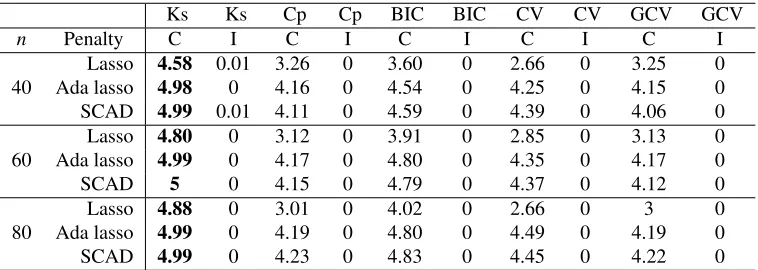
Ks Ks Cp Cp BIC BIC CV CV GCV GCV
n Penalty C I C I C I C I C I
Lasso 4.58 0.01 3.26 0 3.60 0 2.66 0 3.25 0
40 Ada lasso 4.98 0 4.16 0 4.54 0 4.25 0 4.15 0
SCAD 4.99 0.01 4.11 0 4.59 0 4.39 0 4.06 0
Lasso 4.80 0 3.12 0 3.91 0 2.85 0 3.13 0
60 Ada lasso 4.99 0 4.17 0 4.80 0 4.35 0 4.17 0
SCAD 5 0 4.15 0 4.79 0 4.37 0 4.12 0
Lasso 4.88 0 3.01 0 4.02 0 2.66 0 3 0
80 Ada lasso 4.99 0 4.19 0 4.80 0 4.49 0 4.19 0
SCAD 4.99 0 4.23 0 4.83 0 4.45 0 4.22 0
Table 2: The average numbers of correctly selected zeros (C) and incorrectly selected zeros (I) for various selection criteria in simulations of Section 5.1. Here ‘Ks’, ‘Cp’, ‘BIC’, ‘CV’ and ‘GCV’ represent the kappa selection criterion, Mallows’Cp, BIC, CV and GCV, respec-tively.
Table 2 shows that the kappa selection criterion yields the largest number of correctly selected zeros in all scenarios, and it yields almost perfect performance for the adaptive lasso and the SCAD. In addition, all selection criteria barely select any incorrect zeros, whereas the kappa selection cri-terion is relatively more aggressive in that it has small chance to shrink some informative variables to zeros when sample size is small. All other criteria tend to be conservative and include some uninformative variables, so the numbers of correctly selected zeros are significantly less than 5.
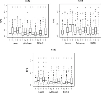
Besides the superior variable selection performance, the kappa selection criterion also delivers accurate prediction performance and yields small relative prediction error as displayed in Figure 1. Note that other criteria, especiallyCp and GCV, produce large relative prediction errors, which could be due to their conservative selection of the informative variables.
K Cp B C G K Cp B C G K Cp B C G
0.0
0.2
0.4
0.6
0.8
1.0
Lasso Adalasso SCAD
RPE
n=40
K Cp B C G K Cp B C G K Cp B C G
0.0
0.2
0.4
Lasso Adalasso SCAD
RPE
n=60
K Cp B C G K Cp B C G K Cp B C G
0.0
0.2
0.4
Lasso Adalasso SCAD
RPE
n=80
Figure 1: Relative prediction errors (RPE) for various selection criteria in simulations of Section 5.1. Here ‘K’, ‘Cp’, ‘B’, ‘C’ and ‘G’ represent the kappa selection criterion, Mallows’
Cp, BIC, CV and GCV, respectively.
per-−2 −1 0 1 2
−1
0
1
Detection
logλ
Kappa Detection
−2 −1 0 1 2
−1
0
1
Sparsity
logλ
Kappa Sparsity
0.00 0.05 0.10 0.15 0.20 0.25 0.30
0.07
0.08
0.09
0.10
0.11
Relative prediction error
α
RPE
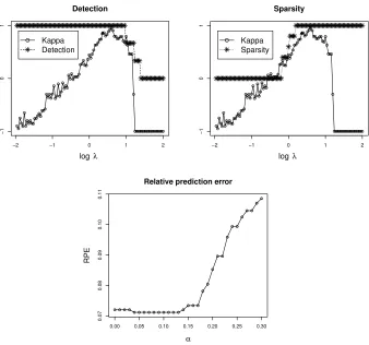
Figure 2: The detection and sparsity of the lasso regression with the kappa selection criterion are shown on the top and the sensitivity ofαto the relative prediction error is shown on the bottom. The optimal log(λ)selected by the kappa selection criterion is denoted as the filled triangle in the detection and sparsity plots.
centage of selecting the truly informative variables, and the sparsity is defined as the percentage of excluding the truly uninformative variables. Figure 2 illustrates the clear relationship between the variable selection stability and the values of detection and sparsity. More importantly, the selection performance of the kappa selection criterion is very stable againstαnwhen it is small. Specifically, we apply the kappa selection criterion on the lasso regression for αn ={100l ; l=0, . . . ,30}and compute the corresponding average RPE over 100 replications. As shown in the last panel of Figure 2, the average RPE’s are almost the same forαn∈(0,0.13), which agrees with the theoretical result in Section 4.
5.2 Scenario II: Diverging pn
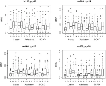
To investigate the effects of the noise level and the dimensionality, we compare all the selection criteria in the diverging pn scenario with a similar simulation model as in Scenario I, except that β= (5,4,3,2,1,0,···,0)T, p
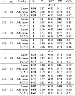
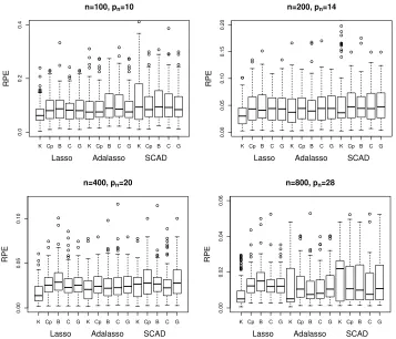
n=100, pn=10; n=200, pn=14; n=400, pn=20; and n=800, pn =28, withσ=1 or 6 respectively. Note that when σ=6, the truly informative variables are much more difficult to detect due to the increased noise level. The percentages of selecting the true active set, the average numbers of correctly selected zeros (C) and incorrectly selected zeros (I), and the relative prediction errors (RPE) are summarized in Tables 3-4 and Figures 3-4.
n pn Penalty Ks Cp BIC CV GCV
σ=1
Lasso 0.98 0.17 0.43 0.10 0.17 100 10 Ada lasso 0.99 0.48 0.86 0.74 0.47 SCAD 0.97 0.47 0.92 0.82 0.47 Lasso 1 0.11 0.49 0.07 0.11 200 14 Ada lasso 1 0.38 0.90 0.66 0.38 SCAD 1 0.46 0.93 0.73 0.47 Lasso 1 0.09 0.53 0.04 0.09 400 20 Ada lasso 1 0.34 0.93 0.73 0.33 SCAD 1 0.43 0.98 0.75 0.43 Lasso 1 0.11 0.51 0.04 0.11 800 28 Ada lasso 1 0.30 0.96 0.74 0.29 SCAD 1 0.46 0.99 0.71 0.46
σ=6
Lasso 0.35 0.14 0.31 0.11 0.15 100 10 Ada lasso 0.21 0.15 0.18 0.11 0.15 SCAD 0.17 0.07 0.12 0.12 0.07 Lasso 0.52 0.10 0.39 0.08 0.09 200 14 Ada lasso 0.40 0.18 0.30 0.16 0.18 SCAD 0.24 0.09 0.15 0.13 0.09 Lasso 0.77 0.10 0.47 0.04 0.10 400 20 Ada lasso 0.53 0.22 0.57 0.24 0.19 SCAD 0.40 0.13 0.30 0.13 0.13 Lasso 0.82 0.07 0.51 0.04 0.06 800 28 Ada lasso 0.68 0.20 0.66 0.37 0.20 SCAD 0.46 0.21 0.39 0.17 0.21
Table 3: The percentages of selecting the true active set for various selection criteria in simulations of Section 5.2. Here ‘Ks’, ‘Cp’, ‘BIC’, ‘CV’ and ‘GCV’ represent the kappa selection criterion, Mallows’Cp, BIC, CV and GCV, respectively.
In the low noise case with σ=1, the proposed kappa selection criterion outperforms other competitors in both variable selection and prediction performance. As illustrated in Tables 3-4, the kappa selection criterion delivers the largest percentage of selecting the true active set among all the selection criteria, and achieves perfect variable selection performance for all the variable selection methods whenn≥200. Furthermore, as shown in Figure 3, the kappa selection criterion yields the smallest relative prediction error across all cases.
As the noise level increases to σ=6, the kappa selection criterion still delivers the largest percentage of selecting the true active set among all scenarios except for the adaptive lasso with
Ks Ks Cp Cp BIC BIC CV CV GCV GCV
n pn Penalty C I C I C I C I C I
σ=1
Lasso 5 0.02 3.25 0 4.20 0 2.95 0 3.25 0
100 10 Ada lasso 5 0.01 4.23 0 4.84 0 4.48 0 4.21 0
SCAD 5 0.03 4.12 0 4.91 0 4.67 0 4.15 0
Lasso 9 0 6.18 0 8.26 0 5.62 0 6.18 0
200 14 Ada lasso 9 0 7.50 0 8.87 0 8.24 0 7.50 0
SCAD 9 0 7.43 0 8.91 0 8.26 0 7.47 0
Lasso 15 0 11.29 0 14.23 0 10.56 0 11.29 0
400 20 Ada lasso 15 0 12.93 0 14.92 0 14.28 0 12.91 0
SCAD 15 0 12.67 0 14.98 0 14.21 0 12.64 0
Lasso 23 0 18.49 0 22.27 0 18.20 0 18.63 0
800 28 Ada lasso 23 0 20.31 0 22.94 0 22.07 0 20.23 0
SCAD 23 0 20.21 0 22.99 0 21.95 0 20.21 0
σ=6
Lasso 4.76 0.57 3.27 0.24 4.31 0.35 3.09 0.20 3.28 0.24 100 10 Ada lasso 4.57 0.77 3.81 0.54 4.62 0.85 3.31 0.49 3.84 0.54 SCAD 4.88 1.22 3.63 0.56 4.37 0.94 3.52 0.58 3.65 0.56 Lasso 8.93 0.43 6.20 0.08 8.32 0.21 5.79 0.07 6.22 0.08 200 14 Ada lasso 8.72 0.55 7.28 0.32 8.69 0.56 7.34 0.37 7.26 0.32 SCAD 9 0.95 7.07 0.37 8.37 0.63 7.25 0.44 7.07 0.37 Lasso 14.98 0.21 11.46 0.03 14.21 0.07 10.60 0.03 11.45 0.03 400 20 Ada lasso 14.88 0.40 12.24 0.09 14.80 0.30 12.93 0.15 12.16 0.09 SCAD 15 0.67 11.97 0.13 14.65 0.51 12.66 0.23 11.88 0.12 Lasso 22.99 0.17 18.65 0.01 22.27 0.01 18.14 0.01 18.68 0.01 800 28 Ada lasso 22.96 0.29 19.84 0.02 22.71 0.16 21.19 0.04 19.71 0.02 SCAD 23 0.55 19.55 0.04 22.73 0.37 20.42 0.11 19.47 0.04
Table 4: The average numbers of correctly selected zeros (C) and incorrectly selected zeros (I) for various selection criteria in simulations of Section 5.2. Here ‘Ks’, ‘Cp’, ‘BIC’, ‘CV’ and ‘GCV’ represent the kappa selection criterion, Mallows’Cp, BIC, CV and GCV, respec-tively.
selection criterion yields the largest number of correctly selection zeros. However, it has relatively higher chance of shrinking the fifth informative variable to zero, while the chance is diminishing as
K Cp B C G K Cp B C G K Cp B C G
0.0
0.1
0.2
0.3
n=100, pn=10
Lasso Adalasso SCAD
RPE
K Cp B C G K Cp B C G K Cp B C G
0.00
0.05
0.10
0.15
n=200, pn=14
Lasso Adalasso SCAD
RPE
K Cp B C G K Cp B C G K Cp B C G
0.00
0.05
0.10
n=400, pn=20
Lasso Adalasso SCAD
RPE
K Cp B C G K Cp B C G K Cp B C G
0.00
0.02
0.04
0.06
n=800, pn=28
Lasso Adalasso SCAD
RPE
Figure 3: Relative prediction errors (RPE) for various selection criteria in Scenario 2 withσ=1. Here ‘K’, ‘Cp’, ‘B’, ‘C’ and ‘G’ represent the kappa selection criterion, Mallows’Cp, BIC, CV and GCV, respectively.
6. Real Application
In this section, we apply the kappa selection criterion to the prostate cancer data (Stamey et al., 1989), which were used to study the relationship between the level of log(prostate specific antigen) (l psa) and a number of clinical measures. The data set consisted of 97 patients who had received a radical prostatectomy, and eight clinical measures were log(cancer volume) (lcavol), log(prostate weight) (lweight),age, log(benign prostaic hyperplasia amount) (lbph), seminal vesicle invasion (svi), log(capsular penetration) (lcp), Gleason score (gleason) and percentage Gleason scores 4 or 5 (pgg45).
The data set is randomly split into two halves: a training set with 67 patients and a test set with 30 patients. Similarly as in the simulated examples, the tuning parameter λ’s are selected through a grid search over 100 grid points{10−2+4l/99; l=0, . . . ,99}on the training set. Since it is unknown whether the clinical measures are truly informative or not, the performance of all the selection criteria are compared by computing their corresponding prediction errors on the test set in Table 5.
predic-K Cp B C G K Cp B C G K Cp B C G
0.0
0.2
0.4
n=100, pn=10
Lasso Adalasso SCAD
RPE
K Cp B C G K Cp B C G K Cp B C G
0.00
0.05
0.10
0.15
0.20
n=200, pn=14
Lasso Adalasso SCAD
RPE
K Cp B C G K Cp B C G K Cp B C G
0.00
0.05
0.10
n=400, pn=20
Lasso Adalasso SCAD
RPE
K Cp B C G K Cp B C G K Cp B C G
0.00
0.02
0.04
0.06
n=800, pn=28
Lasso Adalasso SCAD
RPE
Figure 4: Relative prediction errors (RPE) for various selection criteria in Scenario 2 withσ=6. Here ‘K’, ‘Cp’, ‘B’, ‘C’ and ‘G’ represent the kappa selection criterion, Mallows’Cp, BIC, CV and GCV, respectively.
Penalty Ks Cp BIC CV GCV
Active Lasso 1,2,4,5 1,2,3,4,5,6,7,8 1,2,4,5 1,2,3,4,5,7,8 1,2,3,4,5,6,7,8 Set Ada lasso 1,2,5 1,2,3,4,5 1,2,3,4,5 1,2,3,4,5,6,7,8 1,2,3,4,5
SCAD 1,2,4,5 1,2,3,4,5 1,2,3,4,5 1,2,3,4,5,6,7,8 1,2,3,4,5
Lasso 0.734 0.797 0.734 0.807 0.797
PE Ada lasso 0.806 0.825 0.825 0.797 0.825
SCAD 0.734 0.825 0.825 0.797 0.825
Table 5: The selected active sets and the prediction errors (PE) for various selection criteria in the prostate cancer example. Here ‘Ks’, ‘Cp’, ‘BIC’, ‘CV’ and ‘GCV’ represent the kappa selection criterion, Mallows’Cp, BIC, CV and GCV, respectively.
andsvias the informative variables. As opposed to the sparse regression models produced by other selection criteria, the variableageis excluded by the kappa selection criterion for all base variable selection methods, which agrees with the findings in Zou and Hastie (2005).
7. Discussion
This article proposes a tuning parameter selection criterion based on the concept of variable selec-tion stability. Its key idea is to select the tuning parameter so that the resultant variable selecselec-tion method is stable in selecting the informative variables. The proposed criterion delivers superior numerical performance in a variety of experiments. Its asymptotic selection consistency is also es-tablished for both fixed and diverging dimensions. Furthermore, it is worth pointing out that the idea of stability is general and can be naturally extended to a broader framework of model selection, such as the penalized nonparametric regression (Xue et al., 2010) and the penalized clustering (Sun et al., 2012).
8. Supplementary Material
Lemmas 2 and 3 and their proofs are provided as online supplementary material for this article.
Acknowledgments
The authors thank the Action Editor and three referees for their constructive comments and sugges-tions, which have led to a significantly improved paper.
Appendix A.
The lemma stated below shows that if a variable selection method is selection consistent andεn≺αn, then its variable selection stability converges to 1 in probability.
Lemma 3 Letλ∗nbe as defined in Assumption 1. For anyαn, Psˆ(Ψ,λn∗,m)≥1−αn
≥1−2εn/αn.
Proof of Lemma 3: We denote
A
b∗b 1λ∗n and b
A
∗b2λ∗
n as the corresponding active sets obtained from two sub-samples at theb-th random splitting. Then the estimated variable selection stability based on theb-th splitting can be bounded as
P
ˆ
s∗b(Ψ,λ∗n,m) =1
=P
b
A
∗b 1λ∗n= b
A
∗b2λ∗
n
≥P
b
A
∗b 1λ∗n =
A
T2
≥(1−εn)2≥1−2εn.
By the fact that 0≤sˆ∗b(Ψ,λ∗n,n)≤1, we have
E
ˆ
s(Ψ,λ∗n,m)=E
B−1
B
∑
b=1 ˆ
and 0≤sˆ(Ψ,λ∗
n,n)≤1. Finally, Markov inequality yields that
P1−sˆ(Ψ,λ∗n,m)≥αn
≤
E1−sˆ(Ψ,λ∗ n,m)
αn ≤
2εn αn
,
which implies the desired result immediately.
Proof of Theorem 1:We first show that for anyε>0, lim
n→∞P
ˆ
λn>λ∗norr−n1λnˆ ≤1/ε=0.
Denote Ω1={λn:λn>λn∗}, Ω2={λn:r−n1λn ≤τ} andΩ3={λn:τ≤rn−1λn≤1/ε}, where τ<1/ε,c1(τ)≥1−1/p. It then suffices to show that for anyε>0,
Pˆλn∈Ω1∪Ω2∪Ω3
→0.
First, the definition of ˆλnand Lemma 1 imply that
P(λˆn≤λ∗n)≥P
sˆ(Ψ,λ∗ n,m)
maxλsˆ(Ψ,λ,m) ≥1−αn
≥Psˆ(Ψ,λ∗n,m)≥1−αn
≥1−2εn
αn
.
This, together withεn≺αn, yields that
P
ˆ λn∈Ω1
=P(ˆλn>λ∗n)≤ 2εn
αn → 0.
Next, the definition of ˆλnimplies that
ˆ
s(Ψ,ˆλn,m)≥(1−αn)max
λ sˆ(Ψ,λ,m)≥(1−αn)sˆ(Ψ,λ
∗ n,m).
This, together with Lemma 1, leads to
P
ˆ
s(Ψ,λnˆ ,m)≥1−2αn ≥ P
ˆ
s(Ψ,λnˆ ,m)≥(1−αn)2
≥ P
ˆ
s(Ψ,λ∗n,m)≥1−αn
≥1−2εn
αn,
and hence whenεn≺αn,
Psˆ(Ψ,λˆn,m)≥1−2αn
→1.
Therefore, to showP(λˆn∈Ω2)→0, it suffices to show
P
sup
λn∈Ω2
ˆ
s(Ψ,λn,m)<1−2αn
→1. (13)
But Assumption 2 implies that for any j∈
A
cT and j1∈
A
T, we havePj∈ \
λn∈Ω2
b
A
λ n
≥c1(τ)≥1−
1
p and P
j1∈
\
λn∈Ω2
b
A
λ n
It implies that
lim n→∞P
{1, . . . ,p} ∈ \ λn∈Ω2
b
A
λ n
≥ lim
n→∞1−
∑
j∈Ac T
Pj∈/ \
λn∈Ω2
b
A
λ n
−
∑
j1∈AT
Pj1∈/
\
λn∈Ω2
b
A
λ n
≥ lim
n→∞1− p−p0
p −p0ζn=
p0
p >0.
Since{1, . . . ,p} ∈Tλn∈Ω2
A
b∗bλn implies supλn∈Ω2sˆ∗ b(Ψ,λ
n,m) =−1, then
lim n→∞E
sup
λn∈Ω2 ˆ
s∗b(Ψ,λn,m)
≤1−lim
n→∞P
sup
λn∈Ω2 ˆ
s∗b(Ψ,λn,m) =−1
≤1−p0
p .
In addition, the strong law of large number for U-statistics (Hoeffding, 1961) implies that
B−1
B
∑
b=1 sup
λn∈Ω2 ˆ
s∗b(Ψ,λn,m) a.s.
−→E sup
λn∈Ω2 ˆ
s∗b(Ψ,λn,m)
asB→∞.
Note that supλn∈Ω2sˆ(Ψ,λn,m)≤B−1∑Bb=1supλn∈Ω2sˆ∗b(Ψ,λn,m), it then follows immediately that P(supλn∈Ω2sˆ(Ψ,λn,m)≤1−pp0)→1 and henceP(supλn∈Ω2sˆ(Ψ,λn,m)<1−2αn)→1. Therefore
P(λˆn∈Ω2)→0.
Finally, to showP(λnˆ ∈Ω3)→0, it also suffices to show
P sup
λn∈Ω3
ˆ
s(Ψ,λn,m)<1−2αn
→1. (14)
Assumption 2 implies that for any j∈
A
cT and some j1∈
A
Tc, whennis sufficiently large,P(∩λn∈Ω3{j∈
A
bλn})≥c1(1/ε)>0 and P(∩λn∈Ω3{j1∈/A
bλn})≥c2(τ)>0. Therefore, it follows from the independence between two sub-samples thatP
\
λn∈Ω3
{
A
b∗b1λn6=
A
b ∗b 2λn}
≥ P
\
λn∈Ω3
[
j∈Ac T
{j∈/
A
b∗b1λn,j∈
A
b ∗b 2λn}
≥ P \
λn∈Ω3
{j1∈/
A
b1∗λbn,j1∈A
b∗b 2λn}
= P
\
λn∈Ω3
{j1∈/
A
b1∗λbn}
P
\
λn∈Ω3
{j1∈
A
b2∗λbn}
,
≥ c1(1/ε)c2(τ).
Since the event Tλn∈Ω3{
A
b∗b 1λn 6= bA
∗b2λn} implies that supλn∈Ω3sˆ∗ b(Ψ,λ
n,m) ≤ c3 with c3 = maxA16=A2κ(
A
1,A
2)≤ p−p1 whereA
1,A
2⊂ {1,···,p}, we have, for sufficiently largen,P
sup
λn∈Ω3
ˆ
s∗b(Ψ,λn,m)≤c3
Therefore, for sufficiently largenand anyb>0,
E
sup
λn∈Ω3
ˆ
s∗b(Ψ,λn,m)≤1−c1(1/ε)c2(τ)(1−c3).
Again, by the strong law of large number for U-statistics (Hoeffding, 1961) and the fact that supλn∈Ω3sˆ(Ψ,λn,m)≤B−1∑Bb=1supλn∈Ω3sˆ
∗b(Ψ,λ
n,m), we have
P
sup
λn∈Ω3 ˆ
s(Ψ,λn,m)≤1−c1(1/ε)c2(τ)(1−c3)→1.
For anyε,c1(1/ε)c2(τ)(1−c3)is strictly positive andαn→0, we have
P
sup
λn∈Ω3
ˆ
s(Ψ,λn,m)<1−2αn≥P
sup
λn∈Ω3 ˆ
s(Ψ,λn,m)≤1−c1(1/ε)c2(τ)(1−c3)→1,
and hence(14)is verified andPλˆn∈Ω3
→0.
Combining the above results, we have for anyε>0,
lim n→∞Blim→∞P
rn/ε≤λnˆ ≤λ∗n
=1. (15)
Furthermore, since for anyε>0,
P(
A
bˆλn=
A
T) ≥ Pb
A
ˆλn=
A
T,rn/ε≤ˆλn≤λ∗n
≥ P
\
rn/ε≤λn≤λ∗n
{
A
bλn=
A
T}
+P
rn/ε≤ˆλn≤λ∗n
−1.
Therefore, the desired selection consistency directly follows from(15)and Assumption 1 by letting
ε→0.
Proof of Theorem 2:We prove Theorem 2 by similar approach as in the proof of Theorem 1. For anyε>0, we denoteΩ1={λn:λn>λn∗},Ω2={λn:rn−1λn≤τ}andΩ3={λn:τ≤r−n1λn≤1/ε}, where τ is selected so that τ<1/ε and pn(1−c1n(τ))≻αn. Then we just need to show that
P(λˆn∈Ω1∪Ω2∪Ω3)→0. The probabilityP(λˆn∈Ω1)→0 for anyε>0 can be proved similarly as in Theorem 1.
In addition, Lemma 1 implies thatP(sˆ(Ψ,λ∗n,m)≥1−αn)≥1−2εn/αn, and the definition of ˆ
λnleads toP(sˆ(Ψ,ˆλn,m)≥(1−αn)(1−αn))≥1−2εn/αn, and hence
P
ˆ
s(Ψ,ˆλn,m)≥1−2αn
≥P
ˆ
s(Ψ,λˆn,m)≥(1−αn)(1−αn)
≥1−2εn
αn → 1.
To showP(ˆλn∈Ω2)→0, it suffices to showP(supλn∈Ω2sˆ(Ψ,λn,m)<1−2αn)→1, which can be verified by slightly modifying the proof of(13). Assumption 2a implies that for any j∈
A
cT and
j1∈
A
T, we havePj∈ \
λn∈Ω2
b
A
λ n
≥c1n(τ) and P
j1∈
\
λn∈Ω2
b
A
λ n
As shown in Theorem 1, it implies that
P{1, . . . ,p} ∈ \ λn∈Ω2
b
A
λ n
≥1−(pn−p0n)(1−c1n(τ))−p0nζn,
and henceE(supλn∈Ω2sˆ∗b(Ψ,λn,m))≤1−(pn−p0n)(1−c1n(τ))−p0nζn. By the strong law of large number for U-statistics,
P
sup
λn∈Ω2
ˆ
s(Ψ,λn,m)≤1−(pn−p0n)(1−c1n(τ))−p0nζn
→1.
Therefore,P(supλn∈Ω2sˆ(Ψ,λn,m)<1−2αn)→1 provided thatpn(1−c1n(τ))≻αnandpnζn→0. To showP(ˆλn∈Ω3)→0, it suffices to show
P sup
λn∈Ω3 ˆ
s(Ψ,λn,m)<1−2αn
→1. (16)
Here(16)follows by modifying the proof of(14). According toc4≤(pn−1)/pn, we have
E
sup
λn∈Ω3 ˆ
s∗b(Ψ,λn,m)
≤1−p−n1c1n(1/ε)c2n(τ).
Therefore, following the same derivation as in Theorem 1, we have
P sup
λn∈Ω3 ˆ
s(Ψ,λn,m)≤1−pn−1c1n(1/ε)c2n(τ)
→1.
This, together with the assumptions thatαn≺p−n1c1n(1/ε)c2n(τ)for anyεandτ, leads to the
con-vergence in(16), which completes the proof of Theorem 2.
References
H. Akaike. A new look at the statistical model identification. IEEE Transactions on Automatic Control, 19, 716-723, 1974.
A. Ben-Hur, A. Elisseeff and I. Guyon. A stability based method for discovering structure in clus-tered data.Pacific Symposium on Biocomputing, 6-17, 2002.
P. Breheny and J. Huang. Coordinate descent algorithms for nonconvex penalized regression, with applications to biological feature selection.Annals of Applied Statistics, 5, 232-253, 2011.
J. Cohen. A coefficient of agreement for nominal scales.Educational and Psychological Measure-ment, 20, 37-46, 1960.
P. Craven and G. Wahba. Smoothing noisy data with spline functions: Estimating the correct degree of smoothing by the method of generalized cross-validation.Numerische Mathematik, 31, 317-403, 1979.
J. Fan and R. Li. Variable selection via nonconcave penalized likelihood and its oracle properties.
Journal of the American Statistical Association, 96, 1348-1360, 2001.
J. Fan and R. Li. Statistical Challenges with high dimensionality: Feature selection in knowledge discovery. InProceedings of the International Congress of Mathematicians, 3, 595-622, 2006.
J. Fan and H. Peng. Nonconcave penalized likelihood with a diverging number of parameters.Annals of Statistics, 32, 928-961, 2004.
W. Hoeffding. The strong law of large numbers for U-statistics.Institute of Statistical Mimeograph Series, No. 302, University of North Carolina, 1961.
J. Huang, S. Ma and C.H. Zhang. Adaptive Lasso for sparse high-dimensional regression models.
Statistica Sinica, 18, 1603-1618, 2008.
J. Huang and H. Xie. Asymptotic oracle properties of SCAD-penalized least squares estimators.
IMS Lecture Notes - Monograph Series, Asymptotics: Particles, Processes and Inverse Problems, 55, 149-166, 2007.
C. Mallows. Some comments on Cp.Technometrics, 15, 661-675, 1973.
N. Meinshausen and P. B¨uhlmann. Stability selection.Journal of the Royal Statistical Society, Series B, 72, 414-473, 2010.
G.E. Schwarz. Estimating the dimension of a model.Annals of Statistics, 6, 461-464, 1978.
X. Shen, W. Pan and Y. Zhu. Likelihood-based selection and sharp parameter estimation.Journal of the American Statistical Association, 107, 223-232, 2012.
T.A. Stamey, J.N. Kabalin, J.E. McNeal, I.M. Johnstone, F. Freiha, E.A. Redwine and N. Yang. Prostate specific antigen in the diagnosis and treatment of adenocarcinoma of the prostate: II. Radical prostatectomy treated patients.Journal of Urology, 141, 1076-1083, 1989.
M. Stone. Cross-validatory choice and assessment of statistical predictions. Journal of the Royal Statistical Society, Series B, 36, 111-147, 1974.
W. Sun, J. Wang and Y. Fang. Regularized K-means clustering of high-dimensional data and its asymptotic consistency,Electronic Journal of Statistics, 6, 148-167, 2012.
R. Tibshirani. Regression shrinkage and selection via the Lasso. Journal of the Royal Statistical Society, Series B, 58, 267-288, 1996.
H. Wang and C. Leng. A note on adaptive group Lasso.Computational Statistics and Data Analysis, 52, 5277-5286, 2008.
H. Wang, R. Li and C.L. Tsai. Tuning parameter selectors for the smoothly clipped absolute devia-tion method.Biometrika, 94, 553-568, 2007.
J. Wang. Consistent selection of the number of clusters via cross validation.Biometrika, 97, 893-904, 2010.
L. Xue, A. Qu and J. Zhou. Consistent model selection for marginal generalized additive model for correlated data.Journal of the American Statistical Association, 105, 1518-1530, 2010.
M. Yuan and Y. Lin. Model selection and estimation in regression with grouped variables.Journal of the Royal Statistical Society, Series B, 68, 49-67, 2006.
Y. Zhang, R. Li and C.L. Tsai. Regularization parameter selections via generalized information criterion.Journal of the American Statistical Association, 105, 312-323, 2010.
P. Zhao and B. Yu. On model selection consistency of Lasso.Journal of Machine Learning Research, 7, 2541-2563, 2006.
H. Zou. The adaptive Lasso and its oracle properties.Journal of the American Statistical Associa-tion, 101, 1418-1429, 2006.
H. Zou and T. Hastie. Regularization and variable selection via the elastic net.Journal of the Royal Statistical Society, Series B, 67, 301-320, 2005.
H. Zou, T. Hastie and R. Tibshirani. On the “Degree of Freedom” of the Lasso.Annals of Statistics, 35, 2173-2192, 2007.