Parsimonious Online Learning with Kernels
via Sparse Projections in Function Space
∗Alec Koppel [email protected]
Computational and Information Sciences Directorate U.S. Army Research Laboratory
Adelphi, MD 20783, USA
Garrett Warnell [email protected]
Computational and Information Sciences Directorate U.S. Army Research Laboratory
Adelphi, MD 20783, USA
Ethan Stump [email protected]
Computational and Information Sciences Directorate U.S. Army Research Laboratory
Adelphi, MD 20783, USA
Alejandro Ribeiro [email protected]
Department of Electrical and Systems Engineering University of Pennsylvania
Philadelphia, PA 19104, USA
Editor:Le Song
Abstract
Despite their attractiveness, popular perception is that techniques for nonparametric func-tion approximafunc-tion do not scale to streaming data due to an intractable growth in the amount of storage they require. To solve this problem in a memory-affordable way, we pro-pose an online technique based on functional stochastic gradient descent in tandem with supervised sparsification based on greedy function subspace projections. The method, calledparsimonious online learning with kernels (POLK), provides a controllable tradeoff between its solution accuracy and the amount of memory it requires. We derive conditions under which the generated function sequence converges almost surely to the optimal func-tion, and we establish that the memory requirement remains finite. We evaluate POLK for kernel multi-class logistic regression and kernel hinge-loss classification on three canonical data sets: a synthetic Gaussian mixture model, the MNIST hand-written digits, and the Brodatz texture database. On all three tasks, we observe a favorable trade-off of objec-tive function evaluation, classification performance, and complexity of the nonparametric regressor extracted by the proposed method.
Keywords: kernel methods, online learning, stochastic optimization, supervised learning, orthogonal matching pursuit, nonparametric regression
∗. This work in this paper is supported by NSF CCF-1017454, NSF CCF-0952867, ONR N00014-12-1-0997, ARL MAST CTA, and ASEE SMART. Part of the results in this paper appeared in Koppel et al. (2017).
c
1. Introduction
Reproducing kernel Hilbert spaces (RKHS) provide the ability to approximate functions using nonparametric functional representations. Although the structure of the space is determined by the choice of kernel, the set of functions that can be represented is still suffi-ciently rich so as to permit close approximation of a large class of functions. This resulting expressive power makes RKHS an appealing choice in many learning problems where we want to estimate an unknown function that is specified as optimal with respect to some empirical risk. When learning these optimal function representations in a RKHS, the repre-senter theorem is used to transform the search over functions into a search over parameters, where the number of parameters grows with each new observation that is processed (Whee-den et al., 1977; Norkin and Keyzer, 2009). This growth is what endows the representation with expressive power. However, this growth also results in function descriptions that are as complex as the number of processed observations, and, more importantly, in training algo-rithms that exhibit a cost per iteration that grows with each new iterate (Pontil et al., 2005; Kivinen et al., 2004). The resulting unmanageable training cost renders RKHS learning ap-proaches inefficient for large data sets and outright inapplicable in streaming applications. This is a well-known limitation which has motivated the development of several heuristics to reduce the growth in complexity. These heuristics typically result in suboptimal functional approximations (Richard et al., 2009).
This paper proposes a new technique for learning nonparametric function approxima-tions in a RKHS that respects optimality and ameliorates the complexity issues described above. We accomplish this by: (i) shifting the goal from that of finding an approximation that is optimal to that of finding an approximation that is optimal within a class of par-simonious (sparse) kernel representations; (ii) designing a training method that follows a trajectory of intermediate representations that are also parsimonious. The proposed tech-nique, parsimonious online learning with kernels (POLK), provides a controllable tradeoff between complexity and optimality and we provide theoretical guarantees that neither factor becomes untenable.
Formally, we propose solving expected risk minimization problems, where the goal is to learn a regressor that minimizes a loss function quantifying the merit of a statistical model averaged over a data set. We focus on the case when the number of training examples, N, is either very large, or the training examples arrive sequentially. Further, we assume that these input-output examples, (xn,yn), are i.i.d. realizations drawn from a stationary joint
distribution over the random pair (x,y) ∈ X × Y. This problem class is popular in many fields and particularly ubiquitous in text (Sampson et al., 1990), image (Mairal et al., 2007), and genomic (Ta¸san et al., 2014) processing. Here, we consider finding regressors that are not vector valued parameters, but rather functions f ∈ H in a hypothesized function class
construct the regularized lossR(f) := argminf∈HL(f) + (λ/2)kfk2
H (Shalev-Shwartz et al.,
2010; Evgeniou et al., 2000). We then define the optimal function as
f∗ = argmin
f∈H
R(f) : = argmin
f∈H Ex,y h
`(f x), y
i
+λ 2kfk
2
H (1)
The optimization problem in (1) is intractable in general. However, when H is equipped with areproducing kernel κ:X × X →R, a nonparametric function estimation problem of the form (1) may be reduced to a parametric form via the representer theorem (Wheeden et al., 1977; Norkin and Keyzer, 2009). This theorem states that the optimal argument of (1) is in the span of kernel functions that are centered at points in the given training data set, and it reduces the problem to that of determining the N coefficients of the resulting linear combination of kernels (Section 2). This results in a function description that is data driven and flexible, alas very complex. As we consider problems with larger training sets, the representation of f requires a growing number of kernels (Norkin and Keyzer, 2009). In the case of streaming applications this number would grow unbounded and the kernel matrix as well as the coefficient vector would grow to infinite dimension and an infinite amount of memory would be required to represent f. It is therefore customary to reduce this complexity by forgetting training points or otherwise requiring that f∗ admit a parsi-monious representation in terms of a sparse subset of kernels. This overcomes the difficulties associated with a representation of unmanageable complexity but a steeper difficulty is the
determination of this optimal parsimonious representation as we explain in the following section
1.1. Context
To understand the challenge in determining optimal parsimonious representations, recall that kernel optimization methods borrow techniques from vector valued (i.e., without the use of kernels) stochastic optimization in the sense that they seek to optimize (1) by re-placing the descent direction of the objective with that of a stochastic estimate (Bottou, 1998; Robbins and Monro, 1951). Stochastic optimization is well understood in vector val-ued problems to the extent that recent efforts are concerned with improving convergence properties through the use of variance reduction (Schmidt et al., 2013; Johnson and Zhang, 2013; Defazio et al., 2014), or stochastic approximations of Newton steps (Schraudolph et al., 2007; Bordes et al., 2009; Mokhtari and Ribeiro, 2014, 2015). Stochastic optimization in kernel spaces, however, exhibits two peculiarities that make it more challenging:
i. The implementation of stochastic methods for expected risk minimization in a RKHS requires storage of kernel matrices and weight vectors that together are cubic in the iteration index. This is true even if we require that the solution f∗ admit a sparse representation because, while it may be true that the asymptotic solution admits a sparse representation, the intermediate iterates are not necessarily sparse; see, e.g., Kivinen et al. (2004).
Issue (i) is a key point of departure between kernel stochastic optimization and its vector valued counterpart. It implies that redefiningf∗ to encourage sparsity may make it easier to work with the RKHS representation after it has been learnt. However, the stochastic gradient iterates that need to be computed to find such representation have a complexity that grows with the order of the iteration index (Kivinen et al., 2004), precluding the use of sparsity-encouraging penalties (Fu, 1998). Works on stochastic optimization in a RKHS have variously ignored the intractable growth of the parametric representation of f ∈ H
(Ying and Zhou, 2006; Liu et al., 2008; Pontil et al., 2005; Dieuleveut and Bach, 2014), addressed it indirectly through probabilistic (Rahimi and Recht, 2008, 2009; Dai et al., 2014) or computational (Williams and Seeger, 2001; Zhang et al., 2008) approximations of the kernel, or have augmented the learned function to limit the memory issues associated with kernelization using online sparsification procedures. These approaches focus on limiting the growth of the kernel dictionary through forgetting factors (Kivinen et al., 2004), random dropping (Zhang et al., 2013; Le et al., 2016b), compressive sensing (Engel et al., 2004; Richard et al., 2009; Honeine, 2012), greedy search (Bordes et al., 2005) and projection (Zhao et al., 2012; Zhao and Hoi, 2012; Wang et al., 2012). These approaches overcome Issue (i) but they do so at the cost of dropping optimality [cf. Issue (ii)]. This is because these sparsification techniques introduce a bias in the stochastic gradient which nullifies convergence guarantees, and empirically leads to instability.
Past works that have consideredsupervisedsparsification (addressing issues (i)-(ii)) have only been developed for special cases such as online support vector machines (SVM) (Wang et al., 2012), off-line logistic regression Zhu and Hastie (2005), and off-line SVM (Joachims and Yu, 2009). The works perhaps most similar to ours, but developed only for SVM (Wang et al., 2012)) fixes the number of kernel dictionary elements, or the model order, in advance rather tuning the kernel dictionary to guarantee stochastic descent, i.e. determining which kernel dictionary elements are most important for representingf∗. Further, the analysis of the resulting bias induced by sparsification requires overly restrictive assumptions and is conducted in terms of time-average objective sub-optimality, a looser criterion than almost sure convergence. For specialized classes of loss functions, the bias of the descent direction induced by unsupervised sparsification techniques using random sub-sampling does not prevent the derivation of bounds on the time-average sub-optimality (regret) (Zhang et al., 2013); however, this analysis omits important cases such as support vector machines and kernel ridge regression.
1.2. Contributions
Thus, we project the FSGD iterates onto sparse subspaces, which, rather than being fixed independent of the problem (Zhu et al., 2009), are adaptively constructed from the span of a small number of kernel dictionary elements (Section 3.2). To find these sparse subspaces of the RKHS, we make use of greedy sampling methods based on matching pursuit (Pati et al., 1993). The use of this technique is motivated by: (i) The fact that kernel matrices induced by arbitrary data streams will not, in general, satisfy requisite conditions for methods that enforce sparsity through convex relaxation (Candes, 2008); (ii) That having function iterates that exhibit small model order is of greater importance than exact recovery since SGD iterates are not the goal signal but just a noisy stepping stone to the optimal f∗. Therefore, we construct these instantaneous sparse subspaces by making use of kernel orthogonal matching pursuit (Vincent and Bengio, 2002), a greedy search routine which, given a function and an approximation budget, returns its a sparse approximation and guarantees its output to be in a specific Hilbert-norm neighborhood of its function input. Greedy sampling methods appear in prior works for constructing RKHS subspaces in recursive mini-batching procedures (Keerthi et al., 2006) or with FSGD (Zhao et al., 2012), but in a manner that avoids addressing how to merge greedy compression with obtaining optimal function representations.
To guarantee stochastic descent, we tie the size of the error neighborhood induced by sparse projections to the magnitude of the functional stochastic gradient and other problem parameters, thereby keeping only those kernel dictionary elements necessary for convergence (Section 4). The result is that we are able to conduct stochastic gradient descent using only sparse projections of the stochastic gradient, maintaining a convergence path of moderate complexity towards the optimalf∗(1). When the data and target domains (X and Y, respectively) are compact, for a certain approximation budget depending on the stochastic gradient algorithm step-size, we show that the sparse stochastically projected FSGD sequence still converges almost surely to the optimum of (5) under both attenuating and constant learning rate schemes. Moreover, the model order of this sequence remains finite for a given choice of constant step-size and approximation budget, and is, in the worst-case, comparable to the covering number of the data domain (Zhou, 2002; Pontil, 2003).
In Section 5 we present numerical results on synthetic and empirical data for large-scale kernelized supervised learning tasks. We observe stable convergence behavior of POLK comparable to vector-valued first-order stochastic methods in terms of objective function evaluation, punctuated by a state of the art trade-off between test set error and number of samples processed. Further, the proposed method reduces the complexity of training kernel regressors by orders of magnitude. In Section 6 we discuss our main findings. In particular, we suggest that there is a path forward for kernel methods as an alternative to neural networks that provides a more interpretable mechanism for inference with nonlinear statistical models and that one may achieve high generalization capability without losing convexity, an essential component for efficient training.
2. Statistical Optimization in Reproducing Kernel Hilbert Spaces
Supervised learning is often formulated as an optimization problem that computes a set of parameters θ ∈ Θ to minimize the average of a loss function l : Θ× X × Y → R for training examples (xn,yn) ∈ X × Y. When the number of training examples N is finite,
this goal is referred to asempirical risk minimization (Tewari and Bartlett, 2014), and may be solved using batch optimization techniques. The optimalθis the one that minimizes the regularized average loss, ˜R(θ;{xn, yn}Nn=1) = N1
PN
n=1l(θ; (xn, yn)), over the set of training dataS ={xn, yn}Nn=1, i.e.,
θ∗ = argmin
θ∈Θ ˜
R(θ;S) = argmin
θ∈Θ 1
N
N
X
n=1
l(θ;xn, yn) +
λ
2kθk
2 . (2)
We focus on the case when the inputs are vectors x ∈ X ⊆ Rp and the target domain
Y ⊆ {0,1} in the case of classification orY ⊆Rin the case of regression.
2.1. Supervised Kernel Learning
In the case of supervised kernel learning (M¨uller et al., 2013; Li et al., 2014), Θ is taken to be a Hilbert space, denoted here asH. Elements ofHarefunctions,f :X → Y, that admit a representation in terms of elements of X when H has a special structure. In particular, equipH with a uniquekernel function,κ:X × X →R, such that:
(i) hf, κ(x,·))iH=f(x) for all x∈ X , (ii) H= span{κ(x,·)} for all x∈ X . (3)
whereh·,·iH denotes the Hilbert inner product forH. We further assume that the kernel is
positive semidefinite, i.e. κ(x,x0)≥0 for allx,x0 ∈ X. Function spaces with this structure are called reproducing kernel Hilbert spaces (RKHS).
In (3), property (i) is called the reproducing property of the kernel, and is a consequence of the Riesz Representation Theorem (Wheeden et al., 1977). Replacingf byκ(x0,·) in (3) (i) yields the expression hκ(x0,·), κ(x,·)iH = κ(x,x0), which is the origin of the term
“re-producing kernel.” This property provides a practical means by which to access a nonlinear transformation of the input spaceX. Specifically, denote byφ(·) a nonlinear map of the fea-ture space that assigns to eachxthe kernel functionκ(·,x). Then the reproducing property of the kernel allows us to write the inner product of the image of distinct feature vectorsx
andx0 under the mapφin terms of kernel evaluations only: hφ(x), φ(x0)iH=κ(x,x0). This
is commonly referred to as the kernel trick, and it provides a computationally efficient tool for learning nonlinear functions.
Moreover, property (3) (ii) states that any function f ∈ H may be written as a linear combination of kernel evaluations. For kernelized and regularized empirical risk minimiza-tion, the Representer Theorem (Kimeldorf and Wahba, 1971; Sch¨olkopf et al., 2001) estab-lishes that the optimalf in the hypothesis function classHmay be written as an expansion of kernel evaluations only at elements of the training set as
f(x) =
N
X
n=1
where w = [w1,· · ·, wN]T ∈ RN denotes a set of weights. The upper summand index
N in (4) is henceforth referred to as the model order. Common choices κ include the polynomial kernel and the radial basis kernel, i.e., κ(x,x0) = xTx0+bc and κ(x,x0) =
expn−kx−x0k22
2c2
o
, respectively, where x,x0 ∈ X.
We may now formulate the kernel variant of the empirical risk minimization problem as the one that minimizes the loss functional L:H × X × Y →Rplus a complexity-reducing penalty. The loss functional L may be written as an average over instantaneous losses
`:H × X × Y → R, each of which penalizes the average deviation between f(xn) and the
associated output yn over the training setS. We denote the data loss and complexity loss
asR:H →R, and consider the problem
f∗ = argmin
f∈H
R(f;S) = argmin
f∈H
1
N
N
X
n=1
`(f(xn), yn) +
λ
2kfk 2
H. (5)
The above problem, referred to as Tikhonov regularization (Evgeniou et al., 2000), is one in which we aim to learn a general nonlinear relationship between xn and yn through a
functionf. Throughout, we assume`is convex with respect to its first argumentf(x). By substituting the Representer Theorem expansion in (4) into (5), the optimization problem amounts to finding an optimal set of coefficientsw as
f∗ = argmin
w∈RN
1
N
N
X
n=1
`(
N
X
m=1
wmκ(xm,xn), yn) +
λ
2k
N
X
n,m=1
wnwmκ(xm,xn)k2H
= argmin
w∈RN
1
N
N
X
n=1
`(wTκX(xn), yn) +
λ
2w
TK
X,Xw (6)
where we have defined the Gram matrix (variously referred to as thekernel matrix)KX,X∈
RN×N, with entries given by the kernel evaluations between xm and xn as [KX,X]m,n =
κ(xm,xn). We further define the vector of kernel evaluationsκX(·) = [κ(x1,·). . . κ(xN,·)]T,
which are related to the kernel matrix as KX,X = [κX(x1). . .κX(xN)]. The dictionary of
training points associated with the kernel matrix is defined as X= [x1, . . . ,xN].
Observe that by exploiting the Representer Theorem, we transform a nonparametric infinite dimensional optimization problem in H(5) into a finite N-dimensional parametric problem (6). Thus, for empirical risk minimization, the RKHS provides a principled frame-work to solve nonparametric regression problems as via search over RN for an optimal set
of coefficients. A motivating example is presented next to clarify the setting of supervised kernel learning.
Example 1 (Kernel Logistic Regression) Consider the case of kernel logistic regression
(KLR), with feature vectors xn ∈ X ⊆Rp and binary class labels yn ∈ {0,1}. We seek to
learn a function f ∈ H that allows us to best approximate the distribution of an unknown class label given a training examplex under the assumed model
P(y= 0 |x) = exp{f(x)}
In classical logistic regression, we assume that f is linear, i.e.,f(x) =cTx+b. In KLR, on the other hand, we instead seek a nonlinear function of the form given in (4). By making use of (7) and (4), we may formulate a maximum-likelihood estimation (MLE) problem to find the optimal function f on the basis of S by solving for the w that maximizes the
λ-regularized average negative log likelihood overS, i.e.,
f∗ = argmin
f∈H 1 N N X n=1
−logP(y=yn |x=xn) +
λ
2kfk 2 H (8) = argmin f∈H 1 N N X n=1
log (1 + exp{f(xn)})−1(yn= 1)−f(xn)1(yn= 0) +
λ
2kfk 2
H
= argmin
w∈RN
1 N N X n=1
log 1+exp{wTκX(xn)}
−1(yn= 1)−wTκX(xn)1(yn= 0)+
λ
2w
TK
X,Xw
,
where 1(·) represents the indicator function. Solving (8) amounts to finding a function f
that, given a feature vector x and the model outlined by (7), best represents the class-conditional probabilities that the corresponding label y is either 0 or 1.
2.2. Online Kernel Learning
The goal of this paper is to solve problems of the form (5) when training examples (xn,yn)
either become sequentially available or their total number is not necessarily finite. To do so, we consider the case where (xn,yn) are independent realizations from a stationary joint
distribution of the random pair (x,y) ∈ X × Y (Slavakis et al., 2013). In this case, the objective in (5) may be written as an expectation over this random pair as
f∗= argmin
f∈H
R(f) : = argmin
f∈H Ex,y
[`(f(x), y)] + λ 2kfk
2
H (9)
=argmin
w∈RI
Ex,y[`(
X
n∈I
wnκ(xn,x), y)] +
λ
2k
X
n,m∈I
wnwmκ(xm,xn)k2H .
where we define the average loss as L(f) := Ex,y[`(f(x), y)]. In the second equality in (1),
we substitute in the expansion of f given by the Representer Theorem generalized to the infinite sample-size case established in (Norkin and Keyzer, 2009), withIas some countably infinite indexing set.
3. Algorithm Development
the resulting parametric updates require memory storage whose complexity is cubic in the iteration index (the curse of kernelization), which rapidly becomes unaffordable. To alleviate this memory explosion, we introduce our sparse stochastic projection scheme based upon kernel orthogonal matching pursuit in Section 3.2.
3.1. Functional Stochastic Gradient Descent
Following Kivinen et al. (2004), we derive the generalization of the stochastic gradient method for the RKHS setting. The resulting procedure is referred to asfunctional stochastic gradient descent (FSGD). First, given an independent realization (xt, yt) of the random pair
(x, y), we compute the stochastic functional gradient (Frech´et derivative) ofL(f), stated as
∇f`(f(xt), yt)(·) =
∂`(f(xt), yt)
∂f(xt)
∂f(xt)
∂f (·) (10)
where we have applied the chain rule. Now, define the short-hand notation `0(f(xt), yt) :=
∂`(f(xt), yt)/∂f(xt) for the derivative of`(f(xt), yt) with respect to its first scalar argument
f(xt) evaluated atxt. To evaluate the second term on the right-hand side of (10),
differen-tiate both sides of the expression defining the reproducing property of the kernel [cf. (3)(i)] with respect tof to obtain
∂f(xt)
∂f =
∂hf, κ(xt,·))iH
∂f =κ(xt,·) (11)
With this computation in hand, we present the stochastic gradient method for the kernelized
λ-regularized expected risk minimization problem in (1) as
ft+1 = (1−ηtλ)ft−ηt∇f`(ft(xt), yt) = (1−ηtλ)ft−ηt`0(ft(xt), yt)κ(xt,·), (12)
whereηt>0 is an algorithm step-size either chosen as diminishing with O(1/t) or a small
constant – see Section 4. We further require that, givenλ >0, the step-size satisfiesηt<1/λ
and the sequence is initialized as f0 = 0 ∈ H. Given this initialization, by making use of the Representer Theorem (4), at time t, the functionft may be expressed as an expansion
in terms of feature vectorsxt observed thus far as
ft(x) =
t−1
X
n=1
wnκ(xn,x) =wTtκXt(x). (13)
On the right-hand side of (13) we have introduced the notation Xt = [x1, . . . ,xt−1] ∈
Rp×(t−1) and κXt(·) = [κ(x1,·), . . . , κ(xt−1,·)]T. Moreover, observe that the kernel expan-sion in (13), taken together with the functional update (12), yields the fact that performing the stochastic gradient method in H amounts to the following parametric updates on the kernel dictionaryX and coefficient vectorw:
Xt+1 = [Xt, xt], wt+1= [(1−ηtλ)wt, −ηt`0(ft(xt), yt)], (14)
Observe that this update causes Xt+1 to have one more column than Xt. We define the model order as number of data pointsMtin the dictionary at timet(the number of columns
3.2. Model Order Control via Stochastic Projection
To mitigate the model order issue described above, we shall generate an approximate se-quence of functions by orthogonally projecting functional stochastic gradient updates onto subspacesHD⊆ Hthat consist only of functions that can be represented using some
dictio-nary D= [d1, . . . , dM]∈Rp×M, i.e., HD ={f : f(·) =PMn=1wnκ(dn,·) =wTκD(·)}=
span{κ(dn,·)}Mn=1. For convenience we have defined [κD(·) = κ(d1,·). . . κ(dM,·)], and
KD,D as the resulting kernel matrix from this dictionary. We will enforce parsimony in
function representation by selecting dictionaries D thatMtt.
We first show that, by selecting D =Xt+1 at each iteration, the sequence (12) derived in Section 3.1 may be interpreted as carrying out a sequence of orthogonal projections. To see this, rewrite (12) as the quadratic minimization
ft+1= argmin
f∈H f−
(1−ηtλ)ft−ηt∇f`(ft(xt), yt)
2
H
= argmin
f∈HXt+1
f −
(1−ηtλ)ft−ηt∇f`(ft(xt), yt)
2
H, (15)
where the first equality in (15) comes from ignoring constant terms which vanish upon differentiation with respect to f, and the second comes from observing that ft+1 can be represented using only the points Xt+1, using (14). Notice now that (15) expressesft+1 as the orthogonal projection of the update (1−ηtλ)ft−ηt∇f`(ft(xt), yt) onto the subspace
defined by dictionary Xt+1.
Rather than select dictionary D = Xt+1, we propose instead to select a different dic-tionary, D = Dt+1, which is extracted from the data points observed thus far, at each iteration. The process by which we select Dt+1 will be discussed shortly, but is of dimen-sion p×Mt+1, with Mt+1 t. As a result, we shall generate a function sequence ft that
differs from the functional stochastic gradient method presented in Section 3.1. The func-tionft+1 is parameterized by dictionaryDt+1 and weight vectorwt+1. We denote columns
of Dt+1 as dn for n= 1, . . . , Mt+1, where the time index is dropped for notational clarity
but may be inferred from the context.
To be specific, we propose replacing the update (15) in which the dictionary grows at each iteration by the stochastic projection of the functional stochastic gradient sequence onto the subspaceHDt+1 = span{κ(dn,·)}Mn=1t+1 as
ft+1 = argmin
f∈HDt+1
f −
(1−ηtλ)ft−ηt∇f`(ft(xt), yt)
2
H
:=PHDt+1
h
(1−ηtλ)ft−ηt∇f`(ft(xt), yt)
i
. (16)
where we define the projection operator P onto subspaceHDt+1 ⊂ H by the update (16).
Coefficient update The update (16), for a fixed dictionary Dt+1 ∈Rp×Mt+1, may be
expressed in terms of the parameter space of coefficients only. In order to do so, we first define the stochastic gradient update without projection, given function ft parameterized
by dictionaryDt and coefficientswt, as
˜
This update may be represented using dictionary and weight vector
˜
Dt+1 = [Dt, xt], w˜t+1= [(1−ηtλ)wt, −ηt`0(ft(xt), yt)]. (18)
Observe that ˜Dt+1 has ˜M =Mt+ 1 columns, which is also the length of ˜wt+1. For a fixed dictionary Dt+1, the stochastic projection in (16) amounts to a least-squares problem on the coefficient vector. To see this, make use of the Representer Theorem to rewrite (16) in terms of kernel expansions, and that the coefficient vector is the only free parameter to write
argmin
w∈RMt+1
1 2ηt
Mt+1 X n=1
wnκ(dn,·)−
˜
M
X
m=1 ˜
wmκ(˜dm,·)
2 H (19) = argmin
w∈RMt+1
1 2ηt
Mt+1
X
n,n0=1
wnwn0κ(dn,dn0)−2
Mt+1,M˜
X
n,m=1
wnw˜mκ(dn,d˜m)+
˜
M
X
m,m0=1 ˜
wmw˜m0κ(˜dm,d˜m0)
= argmin
w∈RMt+1
1 2ηt
wTKDt+1,Dt+1w−2wTKDt+1,Dt+1˜ w˜t+1+ ˜wt+1KDt+1˜ ,Dt+1˜ w˜t+1
:=wt+1 .
In (19), the first equality comes from expanding the square, and the second comes from defining the cross-kernel matrix KDt+1,Dt+1˜ whose (n, m)th entry is given by κ(dn,d˜m).
The other kernel matrices KDt+1˜ ,Dt+1˜ and KDt+1,Dt+1 are similarly defined. Note that Mt+1 is the number of columns in Dt+1, while ˜M = Mt+ 1 is the number of columns in
˜
Dt+1 [cf. (18)]. The explicit solution of (19) may be obtained by noting that the last term is a constant independent of w, and thus by computing gradients and solving for wt+1 we obtain
wt+1=K−Dt+1Dt+11 KDt+1Dt+1˜ w˜t+1 , (20)
Given that the projection of ˜ft+1 onto the stochastic subspaceHDt+1, for a fixed dictionary
Dt+1, amounts to a simple least-squares multiplication, we turn to detailing how the kernel dictionary Dt+1 is selected from the data sample path {xu, yu}u≤t.
Dictionary Update The selection procedure for the kernel dictionary Dt+1 is based upon greedy sparse approximation, a topic studied extensively in the compressive sensing community (Needell et al., 2008). The function ˜ft+1= (1−ηt)ft−ηt∇f`(ft;xt,yt) defined
by stochastic gradient method without projection is parameterized by dictionary ˜Dt+1 [cf. (18)], whose model order is ˜M = Mt+ 1. We form Dt+1 by selecting a subset of Mt+1 columns from ˜Dt+1that are best for approximating ˜ft+1in terms of error with respect to the Hilbert norm. As previously noted, numerous approaches are possible for seeking a sparse representation. We make use ofkernel orthogonal matching pursuit (KOMP) (Vincent and Bengio, 2002) with allowed error tolerancet to find a kernel dictionary matrixDt+1 based on the one which adds the latest sample point ˜Dt+1. This choice is due to the fact that we can tune its stopping criterion to guarantee stochastic descent, and guarantee the model order of the learned function remains finite – see Section 4 for details. Similar ideas have independently appeared in a prior work but without any analysis Zhao et al. (2012).
Algorithm 1 Destructive Kernel Orthogonal Matching Pursuit (KOMP)
Require: function ˜f defined by dict. ˜D∈Rp×M˜
, coeffs. ˜w∈RM˜, approx. budget t>0
initializef = ˜f, dictionaryD= ˜D with indicesI, model orderM = ˜M, coeffs. w= ˜w.
while candidate dictionary is non-empty I 6=∅ do
forj= 1, . . . ,M˜ do
Find minimal approximation error with dictionary elementdj removed
γj = min
wI\{j}∈RM−1
kf˜(·)− X
k∈I\{j}
wkκ(dk,·)kH.
end for
Find dictionary index minimizing approximation error: j∗ = argminj∈Iγj
if minimal approximation error exceeds threshold γj∗ > t stop
else
Prune dictionaryD←DI\{j∗}
Revise setI ← I \ {j∗}and model orderM ←M−1.
Compute updated weights wdefined by current dictionary D
w= argmin
w∈RM
kf˜(·)−wTκD(·)kH
end end while
return f,D,w of model orderM ≤M˜ such that kf−f˜kH≤t
Algorithm 1. This flavor of KOMP takes as an input a candidate function ˜f of model order ˜M parameterized by its kernel dictionary ˜D∈Rp×M˜ and coefficient vector ˜w∈RM˜.
The method then seeks to approximate ˜f by a parsimonious function f ∈ H with a lower model order. Initially, this sparse approximation is the original function f = ˜f so that its dictionary is initialized with that of the original function D = ˜D, with corresponding coefficients w = ˜w. Then, the algorithm sequentially removes dictionary elements from the initial dictionary ˜D, yielding a sparse approximation f of ˜f, until the error threshold
kf −f˜kH≤t is violated, in which case it terminates.
At each stage of KOMP, a single dictionary element j of D is selected to be removed which contributes the least to the Hilbert-norm approximation error minf∈HD\{j}kf˜−fkHof the original function ˜f, when dictionaryDis used. Since at each stage the kernel dictionary is fixed, this amounts to a computation involving weightsw∈RM−1 only; that is, the error
of removing dictionary point dj is computed for each j as γj = minwI\{j}∈RM−1kf˜(·)−
P
k∈I\{j}wkκ(dk,·)k. We use the notation wI\{j} to denote the entries of w ∈ RM
re-stricted to the sub-vector associated with indices I \ {j}. Then, we define the dictio-nary element which contributes the least to the approximation error as j∗ = argminjγj.
Algorithm 2 Parsimonious Online Learning with Kernels (POLK)
Require: {xt,yt, ηt, t}t=0,1,2,...
initialize f0(·) = 0,D0 = [],w0= [], i.e. initial dictionary, coefficient vectors are empty
for t= 0,1,2, . . .do
Obtain independent training pair realization (xt, yt)
Compute unconstrained functional stochastic gradient step [cf. (17)]
˜
ft+1(·) = (1−ηtλ)ft−ηt`0(ft(xt),yt)κ(xt,·)
Revise dictionary ˜Dt+1 = [Dt, xt] and weights ˜wt+1 ←[(1−ηtλ)wt, −ηt`0(ft(xt), yt)]
Compute sparse function approximation via Algorithm 1
(ft+1,Dt+1,wt+1) =KOMP( ˜ft+1,D˜t+1,w˜t+1, t)
end for
w= argminw∈RMkf˜(·)−w
Tκ
D(·)kH, and the process repeats as long as the current function
approximation is defined by a nonempty dictionary.
With Algorithm 1 stated, we may summarize the key steps of the proposed method in Algorithm 2 for solving (1) while maintaining a finite model order, thus breaking the “curse of kernelization.” The method, Parsimonious Online Learning with Kernels (POLK), executes the stochastic projection of the functional stochastic gradient iterates onto sparse subspaces HDt+1 stated in (16). The initial function is set to null f0 = 0, meaning that it has empty kernel dictionary D0 = [] and coefficient vector w0 = []. The notation [] is used to denote the empty matrix or vector respective size p×0 or 0. Then, at each step, given an independent training example (xt, yt) and step-size ηt, we compute the unconstrained
functional stochastic gradient iterate ˜ft+1(·) = (1−ηtλ)ft−ηt`0(ft(xt),yt)κ(xt,·) which
admits the parametric representation ˜Dt+1 and ˜wt+1 as stated in (18). These parameters are then fed into KOMP with approximation budget t, such that (ft+1,Dt+1,wt+1) = KOMP( ˜ft+1,D˜t+1,w˜t+1, t).
In the next section, we discuss the analytical properties of Algorithm 2 for solving online nonparametric regression problems of the form (1). We close here with an example algorithm derivation for the kernel logistic regression problem stated in Example 1 and a remark regarding the selection of KOMP to execute the greedy compression.
Example 2 (Kernel Logistic Regression)Returning to the case of kernel logistic regression stated in Example 1, with feature vectorsxn∈ X ⊆Rp and binary class labelsyn∈ {0,1},
we may perform sparse function estimation in H that fits a a training example x to its associated label y under the logistic model [cf. (7)] of the odds-ratio of the given class label. The associatedλ-regularized maximum-likelihood estimation (MLE) is given as (8). Provided that a particular kernel map κ(·,·), regularizer λ, and step-size ηt have been
chosen, the only specialization of Algorithm 2 to this case is the computation of ˜ft, which
example (xt, yt). Doing so specializes (17) to
˜
ft+1(·) = (1−ηtλ)ft−ηt
exp{−f˜t(xt)}
[1 + exp{−f˜t(xt)}]2
κ(xt,·). (21)
The resulting dictionary and parameter updates implied by (21), given in (18), are then fed into KOMP (Algorithm 1) which returns their greedy sparse approximation for a fixed budget t.
Remark 1 (On the Choice of Compression Method)Many penalty-based compression meth-ods (Fu, 1998; Zou and Hastie, 2005) in principle could be used to reduce the complexity of the nonparametric regressor through the introduction of sparsity-promiting terms that are added to the objective in (1). However, given the infinite sample size setting of the problem considered in this work, it is not enough to sparsify the solution, since (1) must be solved with FSGD [cf. (12)]. The per-iteration complexity of FSGD [cf. (14)] that is necessary to actually solve the optimization problem means that it will still be unten-ably computationally burdensome even to find a sparsified solution. Thus, it is necessary to apply sparsification in an online manner to the FSGD sequence, akin to Algorithm 2. However, compressing the FSGD sequence may violate the descent properties of the opti-mization algorithm, which motivates us to address how to compress the parameterization while preserving stochastic descent. In POLK, this is done by identifying the relationship between the projected and un-projected stochastic gradient, and noting that the directional error in this relationship may be controlled by tying compression budgett to the choice of
algorithm learning rateηt.
Therefore, to ensure that we actually attain the minimizer of the expected risk functional (1) almost surely, we need to sparsify FSGD while preserving the validity of the descent direction in the function space. In principle, it is possible to do this with any method that sparsifies FSGD while guaranteeing the function sequence moves in a Hilbert-norm error neighborhood of the true functional stochastic gradient. The reason we select KOMP in particular is that it easily admits a Hilbert-norm error neighborhood stopping criterion in conjunction with its compression procedure, and we were not aware of lower complexity alternatives that meet this stringent criterion. The result is that the complexity of the function sequence is then tailored to solve the learning task at hand and the model order is directly modified on the fly by that which is necessary to represent f∗, rather than arbitrarily fixed in advance of training.
4. Convergence Analysis
We turn to studying the theoretical performance of Algorithm 2 developed in Section 3. In particular, we establish that the method, when a diminishing step-size is chosen, is guaranteed to converge to the optimum of (1). We further obtain that when a sufficiently small constant step-size is chosen, the limit infimum of the iterate sequence is within a neighborhood of the optimum. In both cases, the convergence behavior depends on the approximation budget used in the online sparsification procedure detailed in Algorithm 1.
We also perform a worst-case analysis of the model order of the instantaneous iterates resulting from Algorithm 2, and show that asymptotically the model order depends on that of the optimal f∗ ∈ H. Before proceeding with the analysis, we define key quantities to simplify the analysis and introduce standard assumptions which are necessary to establish convergence. First, define the regularized stochastic functional gradient as
ˆ
∇f`(ft(xt), yt) =∇f`(ft(xt), yt) +λft (22)
Further define the projected stochastic functional gradient associated with the update in (16) as
˜
∇f`(ft(xt), yt) =
ft− PHDt+1
h
ft−ηt∇ˆf`(ft(xt), yt)
i
/ηt (23)
such that the Hilbert space update of Algorithm 2 [cf. (16)] may be expressed as a stochastic descent using projected functional gradients
ft+1 =ft−ηt∇˜f`(ft(xt), yt). (24)
The definitions (23) - (22) will be used to analyze the convergence behavior of the algorithm. Before doing so, observe that the stochastic functional gradient in (22), based upon the fact that (xt, yt) are independent and identically distributed realizations of the
random pair (x, y), is an unbiased estimator of the true functional gradient of the regularized expected risk R(f) in (1), i.e.
E[ ˆ∇f`(ft(xt), yt)
Ft] =∇fR(ft) (25)
for all t. Next, we formally state technical conditions on the loss functions, data domain, and stochastic approximation errors that are necessary to establish convergence.
Assumption 1 The feature spaceX ⊂Rp and target domain Y ⊂Rare compact, and the
reproducing kernel map may be bounded as
sup
x∈X
p
κ(x,x) =X <∞ (26)
Assumption 2 The instantaneous loss ` : H × X × Y → R is uniformly C-Lipschitz
continuous for all z∈R for a fixed y∈ Y
|`(z, y)−`(z0, y)| ≤C|z−z0| (27)
Assumption 4 Let Ft denote the sigma algebra which measures the algorithm history for times u < t, i.e. Ft ={xu, yu, uu}tu=1. The projected functional gradient of the regularized
instantaneous risk in (22) has finite conditional second moments for each t, that is,
E[k∇˜f`(ft(xt), yt)k2H| Ft]≤σ2 (28)
Assumption 1 holds in most practical settings by the data domain itself, and justifies the bounding of the loss in Assumption 2. Taken together, these conditions permit bounding the optimal function f∗ in the Hilbert norm, and imply that the worst-case model order is guaranteed to be finite. Variants of Assumption 2 appear in the analysis of stochastic descent methods in the kernelized setting (Pontil et al., 2005; Ying and Zhou, 2006). As-sumption 3 is satisfied for supervised learning problems such as logistic regression, support vector machines with the square-hinge-loss, the square loss, among others. Moreover, it is a standard condition in the analysis of descent methods (see Boyd and Vanderberghe (2004)). Assumption 4 is common in stochastic approximation literature, and ensures that the variance of the stochastic approximation error is finite. Under these conditions, we establish technical results in Appendix A which are used to establish our main convergence results in the following subsection.
4.1. Iterate Convergence
As is customary in the analysis of stochastic algorithms, we establish that under a dimin-ishing algorithm step-size scheme (non-summable and square-summable), with the sparse approximation budget selection
∞ X
t=1
ηt=∞,
∞ X
t=1
ηt2<∞, t=ηt2, (29)
Algorithm 2 converges exactly to the optimal functionf∗ in stated in (1) almost surely. We use the abbreviation a.s. for an event that occurs almost surely, or with probability 1.
Theorem 2 Consider the sequence generated{ft} by Algorithm 2 withf0 = 0, and denote
f∗ as the minimizer of the regularized expected risk stated in (1). Let Assumptions 1-4 hold and suppose the step-size rules and approximation budget are diminishing as in (29) with regularizer such thatηt<1/λfor allt. Then the objective function error sequence converges to null in infimum almost surely as
lim inf
t→∞ R(ft)−R(f
∗) = 0 a.s. (30)
Moreover, the sequence of functions {ft} converges almost surely to the optimumf∗ as
lim
t→∞kft−f ∗k2
H= 0 a.s. (31)
Proof: See Appendix B.
The result in Theorem 2 states that when a diminishing algorithm step-size is chosen as, e.g. ηt = O(1/t), and the approximation budget that dictates the size of the sparse
exact convergence to the optimizer of the regularized expected risk in (1). However, in obtaining exact convergence behavior, we require the approximation budget to approach null asymptotically, which means that the model order of the resulting function sequence may grow arbitrarily, unless f∗ is sparse and the magnitude of the stochastic gradient reduces sufficiently quickly, i.e., comparable tot=O(1/t2).
If instead we consider a constant algorithm step-size ηt = η and the approximation
budget t= is chosen as a constant which satisfies t ==O(η3/2), we obtain that the
iterates converge in infimum to a neighborhood of the optimum, as we state next.
Theorem 3 Denote{ft} as the sequence generated by Algorithm 2 withf0 = 0, and denote
f∗ as the minimizer of the regularized expected risk stated in (1). Let Assumptions 1-4 hold, and given regularizer λ >0, suppose a constant algorithm step-size ηt =η is chosen such
thatη <1/λ, and the sparse approximation budget satisfies =Kη3/2=O(η3/2), where K
is a positive scaler. Then the algorithm converges to a neighborhood almost surely as
lim inf
t→∞ kft−f ∗k
H≤
√ η λ
K+pK2+λσ2=O(√η) a.s. (32)
Proof: See Appendix C.
Theorem 3 states that when a sufficiently small constant step-size is used together with a bias tolerance induced by sparsification chosen as = O(η3/2), Algorithm 2 converges in infimum to a neighborhood of the optimum which depends on the chosen step-size, the parsimony constant K which scales the approximation budget , the regularization parameter λ, as well as the variance of the stochastic gradient σ2. This result again is typical of convergence results in stochastic gradient methods. However, the use of a constant learning rate allows use to guarantee the model order of the resulting function sequence is always bounded, as we establish in the following subsection.
4.2. Model Order Control
In this subsection, we establish that the sequence of functions{ft}generated by Algorithm 2, when a constant algorithm step-size is selected, is parameterized by a kernel dictionary which is guaranteed to have finitely many elements, i.e., its the model order remains bounded. We obtain that the worst-case bound on the model order of ft depends by the topological
properties of the feature spaceX, the Lipschitz constant of the instantaneous loss, and the radius of convergence ∆ = (√η/λ)(K+√K2+λσ2) defined in Theorem 3.
Theorem 4 Denote ft as the function sequence defined by Algorithm 2 with constant
step-sizeηt=η <1/λand approximation budget=Kη3/2 whereK >0is an arbitrary positive
scalar. Let Mt be the model order of ft i.e., the number of columns of the dictionary Dt which parameterizesft. Then there exists a finite upper boundM∞ such that, for allt≥0, the model order is always bounded as Mt ≤ M∞. Consequently, the model order of the limiting function f∞= limtft is finite.
Proof: See Appendix D.1.
The number of kernel dictionary elements in the function sequenceftgenerated by
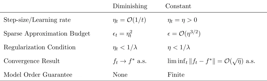
Table 1: Summary of convergence results for different parameter selections.
Diminishing Constant
Step-size/Learning rate ηt=O(1/t) ηt=η >0
Sparse Approximation Budget t=η2t =O(η3/2)
Regularization Condition ηt<1/λ η <1/λ
Convergence Result ft→f∗ a.s. lim inftkft−f∗k=O(
√ η) a.s.
Model Order Guarantee None Finite
of the feature space φ(X) = κ(X,·), as shown in the proof of Theorem 4. Moreover, the online sparsification procedure induced by KOMP reduces to a condition on the scale of the packing number of φ(X) as stated in (76). Specifically, as the radius K
√
η
C increases,
the packing number of the kernelized feature space decreases, and hence the required model order to fillφ(X) decreases. This radius depends on the constantKwhich scales the approx-imation budget selectionη, the learning rateη, and the constantC bounding the gradient of the regularized instantaneous loss.
We have established that Algorithm 2 yields convergent behavior for the problem (1) in both diminishing and constant step-size regimes. When the learning rate ηt satisfies ηt <
1/λ, where λ >0 is the regularization parameter, and is attenuating such thatP
tηt=∞
and P
tη2t < ∞, i.e., ηt = O(1/t), the approximation budget t of Algorithm 1 must
satisfyt=ηt2 [cf. (29)]. Practically speaking, this means that asymptotically the iterates
generated by Algorithm 2 may have a very large model order in the diminishing step-size regime, since the approximation budget is vanishing as t =O(1/t2). On the other hand,
when a constant algorithm step-size ηt = η is chosen to satisfy η < 1/λ, then we only
require the constant approximation budgett= to satisfy=O(η3/2). This means that
in the constant learning rate regime, we obtain a function sequence which converges to a neighborhood of the optimal f∗ defined by (1) and is guaranteed to have a finite model order. These results are summarized in Table 1.
Remark 5 (Sparsity of f∗)Algorithm 2 provides a method to avoid keeping an unneces-sarily large number of kernel dictionary elements along the convergence path towardsf∗ [cf. (1)], solving the classic scalability problem of kernel methods in stochastic programming. However, if the optimal function admits a low dimensional representation|I| ∞, then in addition to extracting memory efficient instantaneous iterates, POLK will obtain the opti-mal function exactly. In Section 5, we illustrate this property via a multi-class classification problem where the data is generated from Gaussian mixture models.
4.3. Complexity Analysis
denote the dimension of the input (feature) space. For convenience of analysis, Algorithm 2 can be thought of as operating in two distinct phases:
i. Append: augment the dictionary and weights so as to take the true FSGD step (i.e., such that they represent ˜ft+1).
ii. Prune: use matching pursuit to reduce the model order (i.e., compute the approxi-mationft+1).
In analyzing the append phase, there are two major operations to consider. The first is the computation of the coefficient`0(f(xt), yt) for the new point, which requiresMt kernel
evaluations, {κ(dj,xt)}Mj=1t , to be weighted and summed. Computing the kernel values exhibits complexityO(pM2
t) (the complexity of a kernel evaluation scales at least linearly
with p), and the weighting and summing exhibits complexity O(Mt). The second major
operation that takes place in the append phase is that of augmenting the kernel matrix. However, for computational efficiency, a copy of the inverse of this kernel matrix is also kept, which can be updated in O(Mt2) time using classical rank-one, block-inverse update rules, based on the Sherman-Woodbury-Morrison identity (see, e.g., KRLS in Engel et al. (2004)). Therefore, the total computational complexity of the append phase is O(M2
t).
To analyze the pruning phase, we first introduce some additional notation. LetZtdenote
the total number of the outer iterations of Algorithm 1 that actually take place at time t, i.e., the number of points removed from ˜D. Using an efficient implementation of Algorithm 1 inspired by Vincent and Bengio (2002), each of theseZtiterations exhibits a computational
complexity of O(M2
t). After the stopping criterion has been met, the augmented function
is projected onto the subspace spanned by the pruned dictionary, which also exhibits a complexity of O(Mt2). Finally, the new kernel matrix and its inverse are updated, which, too, incurs a computational cost ofO(M2
t), bringing the overall complexity of the pruning
phase toO(ZtMt2). A pessimistic estimate ofZtisMt, although in practice it is always less
than the mini-batch size B.
Combining the terms from each phase, the total complexity of Algorithm 2 at iteration
t comes out to O(ZtMt2). In the steady-state, Z = 1 (i.e., Mt+1 = Mt), which further
reduces the expression to O(M2
t), exactly the complexity of KRLS (Engel et al., 2004).
Observe that the complexity of FSGD isO(t), which means that POLK is computationally advantageous whenever t > ZtMt2. Since limtMt is guaranteed to be finite, and usually
Zt ≤ B, the mini-batch size.Thus, POLK is justified whenever t is large. This is typical
of the online methods for kernel learning that we compare against experimentally in the following section.
Remark 6 (Cheaper Projections)Both theoretically and in practice, it is possible to cheapen the cost of projections by replacing the argmin in KOMP by a scheme that drops kernel dictionary elementsuniformly at random until the function hits the boundary of a Hilbert-norm error neighborhood. Such a scheme’s convergence would still be guaranteed by the preceding theoretical analysis, and the cost of pruning points would be significantly cheaper. Specifically, it would be at most linear in the dictionary sizeO(MtZt). However, the price
alternatives in the literature adopt a version of this approach, but withfixed subspace sizes (Wang and Vucetic, 2010a; Wang et al., 2012; Zhao and Hoi, 2012; Zhang et al., 2013; Le et al., 2016b; Lu et al., 2016) rather than error-neighborhood budgets, as is done in this work, which is not enough to establish almost sure convergence.
5. Experiments
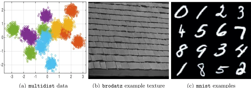
In this section, we evaluate POLK by considering its performance on two supervised learning tasks trained for three streaming data sets. The specific tasks we consider are those of (a) training a multi-class kernel logistic regressor (KLR), and (b) training a multi-class kernel support vector machine (KSVM). The three data sets we use are (i)multidist, a synthetic data set we constructed using two-dimensional Gaussian mixture models; (ii) mnist, the MNIST handwritten digits (Lecun and Cortes, 2009); and (iii) brodatz, image textures drawn from a subset of the Brodatz texture database (Brodatz, 1966).
Where possible, we compare our technique with competing methods. Specifically, for the online support vector machine case, we compare with budgeted stochastic gradient descent (BSGD) Wang et al. (2012), a fixed subspace projection method, which requires a maximum model order a priori; Dual Space Gradient Descent (Dual) (Le et al., 2016a), which executes a hybrid combination of functional stochastic gradient method together with a hybrid random feature representation of the regression function; nonparametric budgeted stochastic gradient descent (NPBSGD) Le et al. (2016b), which combines a fixed subspace projection with random dropping, Naive Online Rreg Minimization Algorithm (NORMA) (Kivinen et al., 2004), which does a greedy objective function value based truncation to a fixed budget, and an instantiation of Budgeted Passive-Aggressive (BPA) algorithm based on k-nearest neighbor merging of incoming points (Wang and Vucetic, 2010a). We note that all the aforementioned methods fix the model order except Dual (Le et al., 2016a). Further, for logistic regression, from the preceding list, we omit BPA and BSGD since they are derived specifically for the SVM setting. We compare all of these online methods on our first data set but then only compare POLK and BSGD on the later benchmark data domains, since the trends we observe for the former directly scale up to the later.
For off-line (batch) KLR, we compare with the import vector machine (IVM) (Zhu and Hastie, 2005), a sparse second-order method. We also compare with the batch techniques of LIBSVM (Chang and Lin, 2011), applicable to KSVM only, an L-BFGS solver (Nocedal, 1980), and methods which approximate the kernel matrix using either Fourier transforms (Rahimi and Recht, 2008, 2009) or Nystr¨om approximation (Williams and Seeger, 2001; Zhang et al., 2008).
5.1. Tasks
The tasks we consider are those of multi-class classification, which is a problem that admits approaches based on probabilistic and geometric criteria. In what follows, we usexn∈ X ⊂
Rp to denote the nth feature vector in a given data set, and yn ∈ {1, . . . , C} to denote its
corresponding label.
particular, define a set of class-specific activation functions fc :X →R, and denote them
jointly as f ∈ HC. In Multi-KSVM, points are assigned the class label of the activation
function that yields the maximum response. KSVM is trained by taking the instantaneous loss` to be the multi-class hinge function which defines the margin separating hyperplane in the kernelized feature space, i.e.,
`(f,xn, yn) = max(0,1 +fr(xn)−fyn(xn)) +λ
C
X
c0=1
kfc0k2H , (33)
wherer = argmaxc06=yfc0(x). Further details may be found in Murphy (2012).
Multi-class Kernel Logistic Regression (Multi-KLR)The second task we consider is that of kernel logistic regression, wherein, instead of maximizing the margin which separates sample points in the kernelized feature space, we instead adopt a probabilistic model on the odds ratio that a sample point has a specific label relative to all others. Using the same notation as above for the class-specific activation functions, we adopt the probabilistic model:
P(y=c|x), Pexp(fc(x))
c0exp(fc0(x))
. (34)
which models the odds ratio of a given sample point being in class c versus all others. We use the negative log likelihood pertaining to the above model as the instantaneous loss (see, e.g., Murphy (2012)), i.e.,
`(f,xn, yn) =−logP(y=yn|xn) +
λ
2
X
c
kfck2H
= log X
c0
exp(fc0(xn))
!
−fyn(xn) +
λ
2
X
c
kfck2H. (35)
Observe that the loss (35) substituted into the empirical risk minimization problem in Example 1 is its generalization to multi-class classification. For a given set of activation functions, the classification decision ˜c for xis given by the class that yields the maximum likelihood, i.e., ˜c= argmaxc∈{1,...,C}fc(x).
5.2. Data Sets
We evaluate Algorithm 2 for the Multi-KLR and Multi-KSVM tasks described above using
themultidist,mnist,brodatz data sets.
multidist
In a manner similar to (Zhu and Hastie, 2005), we generate the multidist data set using a set of Gaussian mixture models. The data set consists N = 5000 feature-label pairs for training and 2500 for testing. Each labelynwas drawn uniformly at random from the label
set. The corresponding feature vector xn ∈ Rp was then drawn from a planar (p = 2),
equitably-weighted Gaussian mixture model, i.e., xy ∼ (1/3) P3
j=1N(µy,j, σy,j2 I) where
σy,j2 = 0.2 for all values of y and j. The means µy,j are themselves realizations of their
-3 -2 -1 0 1 2 3 -2
-1 0 1 2
(a)multidistdata (b) brodatzexample texture (c)mnistexamples
Figure 1: Visualizations of the data sets used in experiments.
{θ1, . . . ,θC} are equitably spaced around the unit circle, one for each class label, and
σ2
y = 1.0. We fix the number of classes C = 5, meaning that the feature distribution has,
in total, 15 distinct modes. The data points are plotted in Figure 1(a).
mnist
The mnist data set we use is the popular MNIST data set (Lecun and Cortes, 2009),
which consists of N = 60000 feature-label pairs for training and 10000 for testing. Feature vectors are p = 784-dimensional, where each dimension captures a single grayscale pixel value (scaled to lie within the unit interval) that corresponds to a unique location in a 28-pixel-by-28-pixel image of a cropped, handwritten digit. Labels indicate which digit is written, i.e., there are C= 10 classes total, corresponding to digits 0, . . . ,9 – examples are given in Figure 1(c).
brodatz
We generated thebrodatzdata set using a subset of the images provided in Brodatz (1966). Specifically, we used 13 texture images (i.e.,C= 13), and from them generated a set of 256 textons (Leung and Malik, 1999). Next, for each overlapping patch of size 24-pixels-by-24-pixels within these images, we took the feature to be the associated p = 256-dimensional texton histogram. The corresponding label was given by the index of the image from which the patch was selected. When then randomly selected N = 10000 feature-label pairs for training and 5000 for testing. An example texture image can be seen in Figure 1(b).
5.3. Parameter Selection
For the choice of kernel, some intuition regarding the data domain is helpful, but typically the Gaussian kernel is a good starting point, and therefore is our selection for all of the experiments. For bandwidth selection ˜σ2, we find that choosing it according to the sample variance of a cross-validation training subset to be reasonably effective, and this strategy was used in our implementation. The mini-batch size of 32 was selected based on reducing the noise of stochastic approximation error once steady state is achieved, and was done through trial and error by starting at batch sizes of 1 and doubling until the computational burden of a mini-batch exceeded its benefits in terms of noise reduction. We find the regularizerλ
it as a small constant. For problems with worse conditioning, however, larger regularizers may be useful.
The selection of the algorithm step-size and parsimony constant in our experiments is done through a simple trial and error procedure. We begin with a small step-size, between 0.01 and 0.1, to test whether the algorithm converges, with parsimony constantK = 0.001. Convergence, however, may occur while the model order grows untenably. So, we progres-sively increase the parsimony constant until the bias in the stochastic gradient becomes unmanageable and the algorithm diverges. We select the parsimony constant to be as large as possible while still preserving convergence of the algorithm. Then, we exploit knowledge of the trade-off between learning rate and step-size selection: smaller step-sizes yield slower learning and smaller asymptotic error. In light of this fact, we increment the step-size to increase the learning rate, and then ramp up the parsimony constant to its maximum value that preserves convergence. This trial and error procedure only needed to be repeated a few times for each data set/problem instance to obtain the POLK results presented in this section.
5.4. Results
For each task and data set described above, we implemented POLK (Algorithm 2) along with the competing methods described at the beginning of the section. For some of the tasks, only a subset of the competing methods are applicable, and in some cases such as online logistic regression, none are. Here, we shall describe the details of each experimental setting and the corresponding results.
multidist Results
Sparse SVM Due to the small size of our synthetic multidist data set, we were able to generate results for the Multi-KSVM task using each of the methods specified earlier except for IVM. For POLK, we used the following specific parameter values: we select the Gaussian/RBF kernel with bandwidth ˜σ2 = 0.6, constant learning rate η= 6.0, parsimony constantK= 0.04, and regularization constantλ= 10−6. Further, we processed streaming samples in mini-batches of size 32. For BSGD, Dual, NORMA, NPBSGD, and BPA, we used the same ˜σ2 andλ, but achieved the best results with smaller constant learning rateη= 1.0 (perhaps due, in part, to the fact that it is unclear how to fold mini-batching into their implementation). For Dual, we set k = 3, which determines the how many model points we search over to omit from the dictionary and instead contribute to the random feature functional representation. For NPBSGD, we set the Bernoulli parameter p = min(1, β/t) with β = (45/70)N as in the experiments of Le et al. (2016b). In order to compare with POLK, we set the competing methods’ pre-specified model orders or budget parameters to be 16, i.e., the steady-state model orders of POLK parameterized with the value of K
specified above.
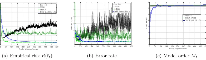
In Figure 2 we plot the empirical results of this experiment for POLK and its competi-tors, and observe that POLK outperforms many of its competitors by an order of magnitude in terms of objective evaluation (Fig. 2(a)) and test-set error rate (Fig 2(b)). The notable exception is NPBSGD which comes close in terms of objective evaluation but still falls short in terms of test error. Moreover, because the marginal feature density of multidist
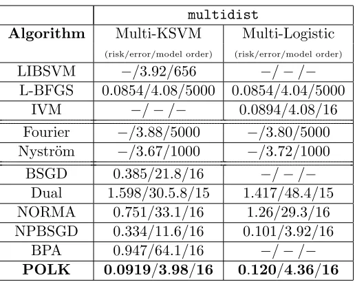
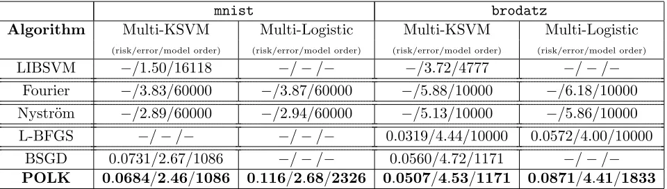
multidist
Algorithm Multi-KSVM Multi-Logistic
(risk/error/model order) (risk/error/model order)
LIBSVM −/3.92/656 −/−/−
L-BFGS 0.0854/4.08/5000 0.0854/4.04/5000 IVM −/−/− 0.0894/4.08/16 Fourier −/3.88/5000 −/3.80/5000 Nystr¨om −/3.67/1000 −/3.72/1000
BSGD 0.385/21.8/16 −/−/−
Dual 1.598/30.5.8/15 1.417/48.4/15 NORMA 0.751/33.1/16 1.26/29.3/16 NPBSGD 0.334/11.6/16 0.101/3.92/16
BPA 0.947/64.1/16 −/−/−
POLK 0.0919/3.98/16 0.120/4.36/16
Table 2: Comparison of different methods on the multidist data set for extracting the optimally sparse functional representation, i.e., K = 0.04 for POLK and M = 16 for online competitors. Reported risk and error values for POLK and BSGD were averaged over the final 5% of processed training examples. Dashes indicate where the method could not be used to generate results because it is not defined for that task. LIBSVM is used as a baseline, but note that it uses a fundamentally different model for multi-class problems (a separate one-vs-all classifier is trained for each class, and then at test time, a majority vote is executed), and so a comparable risk value can not computed.
POLK for K = 0.04 (i.e., MT = 16) (Fig. 2(c)). Several alternatives initialized with this
parameter, on the other hand, do not converge. Observe that for this task POLK exhibits a state of the art trade off between test set accuracy and number of samples processed – reaching below 4% error after only 1249 samples. The final decision surfacefT of this trial
of POLK is shown in Fig. 4(a), where it can be seen that the selected kernel dictionary elements concentrate near the modes of the marginal feature density.
0 500 1000 1500 2000 2500 3000 3500 4000 4500 5000 10-2
10-1 100 101
(a) Empirical riskR(ft)
0 500 1000 1500 2000 2500 3000 3500 4000 4500 5000
0 0.1 0.2 0.3 0.4 0.5 0.6 0.7 0.8 0.9 1
(b) Error rate
0 500 1000 1500 2000 2500 3000 3500 4000 4500 5000 2
4 6 8 10 12 14 16 18 20
(c) Model orderMt
Figure 2: Comparison of POLK and its competitors on the multidist data set for the Multi-KSVM task for extracting a optimally sparse kernel regressor. Observe that POLK achieves lower risk and higher accuracy when we seek to learn a statistical model of comparable complexity to the class-conditional density (M = 15 total modes). Competing methods yield slower learning and higher test-set error rates.
0 500 1000 1500 2000 2500 3000 3500 4000 4500 5000
10-2 10-1 100
(a) Empirical riskR(ft)
0 500 1000 1500 2000 2500 3000 3500 4000 4500 5000 0
0.05 0.1 0.15 0.2 0.25 0.3 0.35 0.4
(b) Error rate
0 500 1000 1500 2000 2500 3000 3500 4000 4500 5000 0
20 40 60 80 100 120 140 160 180 200
(c) Model orderMt
-3 -2 -1 0 1 2 3 -2
-1.5 -1 -0.5 0 0.5 1 1.5 2
(a)fT (hinge loss)
-3 -2 -1 0 1 2 3
-2.5 -2 -1.5 -1 -0.5 0 0.5 1 1.5 2 2.5
(b)fT (logistic loss)
Figure 4: Visualization of the decision surfaces yielded by POLK for the Multi-KSVM and Multi-Logisitic tasks on themultidistdata set. Training examples from distinct classes are assigned a unique color. Grid colors represent the classification decision by fT. Bold black dots are kernel dictionary elements, which concentrate at
the modes of the data distribution. Solid lines are drawn to denote class label boundaries, and dashed lines in 4(b) are drawn to denote confidence intervals.
0 500 1000 1500 2000 2500 3000 3500 4000 4500 5000 100
(a) Empirical riskR(ft)
0 500 1000 1500 2000 2500 3000 3500 4000 4500 5000
0 0.1 0.2 0.3 0.4 0.5 0.6 0.7 0.8 0.9
(b) Error rate
0 500 1000 1500 2000 2500 3000 3500 4000 4500 5000 0
2 4 6 8 10 12 14 16 18 20
(c) Model orderMt
Figure 5: Empirical behavior of the POLK algorithm applied to themultidistdata set for the Multi-Logistic task. Observe that the algorithm converges to a low risk value (R(ft)<10−1) and achieves test set accuracy between 4% and 5% depending on
choice of parsimony constantK, which respectively corresponds to a model order between 75 and 16.
Dense SVM We now repeat the previous experiment with the same parameters except for a different parsimony constant K = 10−4 for POLK and a model order of M = 129 for its competitors, given that this is the value extracted by POLK for this parameter selection. The results of this experiment are given in Figure 3. Observe that NORMA and Dual appear to not converge for this experiment, while POLK converges stably, although its learning rate is exceeded by NPBSGD. This trend is observed both in terms of the risk functional (Fig. 3(a)) and test-set error (Fig 3(b)). We believe NPBSGD performs better for this case due to the smoothness of the logistic loss relative to the hinge loss. However, the test errors of these methods stabilize to similar levels of accuracy (below 4% error rate).
0 500 1000 1500 2000 2500 3000 3500 4000 4500 5000 0
0.2 0.4 0.6 0.8 1 1.2 1.4 1.6 1.8
(a) Empirical riskR(ft)
0 500 1000 1500 2000 2500 3000 3500 4000 4500 5000 0
0.1 0.2 0.3 0.4 0.5 0.6
(b) Error rate
0 500 1000 1500 2000 2500 3000 3500 4000 4500 5000 10
20 30 40 50 60 70 80
(c) Model orderMt
Figure 6: Empirical behavior of the POLK algorithm applied to themultidistdata set for the Multi-Logistic task. Observe that the algorithm converges to a low risk value (R(ft)<10−1) and achieves test set accuracy between 4% and 5% depending on
choice of parsimony constantK, which respectively corresponds to a model order between 75 and 16.
regularization constantλ= 10−6. As in Multi-KSVM, we processed the streaming samples in mini-batches of size 32. The empirical behavior of POLK for the Multi-Logistic task can be seen in Figure 5 and the final decision surface is presented in Figure 4(b). Observe that POLK is exhibits comparable convergence to the SVM problem, but a smoother descent due to the differentiability of the multi-logistic loss. The competing methods, initialized with a model order of M = 16 do not converge, except for NPBSGD, which attains comparable test error to POLK. In Table 2 we present final accuracy and risk values on the logistic task, and note that it performs comparably, or in some cases, favorably, to the batch techniques (IVM, L-BFGS, Random Features, Nystr¨om withk-means sampled points), while processing streaming data. The final model fT extracted by POLK attains comparable performance
to off-line methods while reducing the model complexity by several orders of magnitude.
Dense KLR Now, we re-rerun the previous experiment but modify the parsimony constant of POLK as K = 0.001, which yields a limiting model of order M = 75. The competing methods are then run with this selection. The results of this experiment are given in Figure 6: observe that NORMA and Dual diverge, while NPBSGD converges slightly faster albeit more noisily than POLK. The later two methods attain comparable test accuracy near 96% by the end of training.
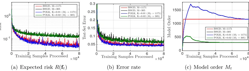
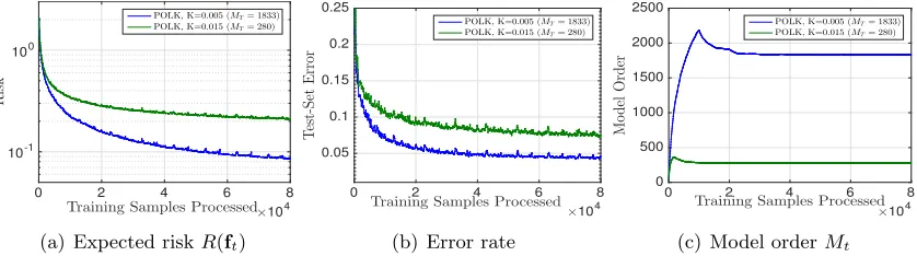
mnist and brodatz Results
By construction, the multidist data set above yields optimal activation functions that are themselves sparse (i.e., f∗ has a low model order due to the marginal feature density). Here, we analyze the performance of POLK on more realistic data sets where the optimal solutions are not sparse, i.e., where one might desire a sparse approximation. Due to the increased size and dimensionality of these data sets, we were unable to generate results for
mnistusing the batch L-BFGS technique, and unable to generate results for either data set
using IVM. With Random Fourier Features onmnist, we use a bandwidth of 0.0095 with