Venting_AALM_Online_Appendix.pdf

(1)

Venting Out: Exports during a Domestic Slump

Miguel Almunia, Pol Antràs, David Lopez-Rodriguez and Eduardo Morales

(2)

C Appendix Figures

C.1 Evolution of the Stock of Vehicles in Spain

FigureC.1plots the evolution of the stock of vehicles per capita in Spain over the period 2002-2013. The figure illustrates the abrupt stop in 2009 of the expansion in that stock during the boom period.

Figure C.1: Stock of Vehicles per Capita (National Average)

Boom period

Bust period

.56

.6

.64

.68

V

e

h

icl

e

s

p

e

r

ca

p

it

a

:

N

a

ti

o

n

a

l A

ve

ra

g

e

2002 2003 2004 2005 2006 2007 2008 2009 2010 2011 2012 2013 Year

C.2 Spatial Distribution of Economic Activity in Spain

Figure C.2plots the 2002-2008 yearly average number of firms and number of exporting firms for each of the 47 Spanish peninsular provinces (see Appendix sectionsB.2and B.3for information on the sources of data).

Figure C.2: Distribution of Economic Activity in Spain: Variation Across Provinces

(3)

C.3 Variation in Domestic Sales and Vehicles per capita at the Municipal Level FigureC.3illustrates variation across 5-digit zip codes in both the boom-to-bust changes in average manufacturing firm-level domestic sales and in the boom-to-bust changes in the number of vehicles per capita. We do so for the case of the two most populated provinces in Spain: Madrid and Barcelona. To facilitate a comparison of the within-province across-zip codes variation illustrated in FigureC.3with the across-province variation illustrated in Figure4of the main text, the average zip code changes illustrated in FigureC.3have been standardized using the Spain-wide mean and cross-province standard deviation used to standardize the corresponding variables in Figure4.

Panels (a) and (b) reveal a large heterogeneity in the change in both firms’ average domestic sales and vehicles per capita across zip codes located in the region of Madrid: while the center area of the region that contains a large number of tightly packed zip codes (this area corresponds to the city of Madrid) experienced small reductions in firm average domestic sales (relative to the mean firm of the average province), surrounding zip codes experienced changes in domestic sales that were more than two standard deviations above the national average. Similarly, while the zip codes belonging to the city of Madrid experienced a large reduction in the number of vehicles per capita (more than two standard deviations smaller than the Spain-wide average), other zip codes to the east, north and west of the city of Madrid saw increases in vehicles per capita significantly above the national average. Panels (c) and (d) provide analogous information for the province of Barcelona. Although the heterogeneity across zip codes located in the province of Barcelona is smaller than that observed within the Madrid region, panel (c) still shows that certain zip codes experienced growth rates smaller than the national average while others experienced changes in firm average domestic sales more than a standard deviation above that average.

C.4 First-Stage and Reduced-Form Relationships

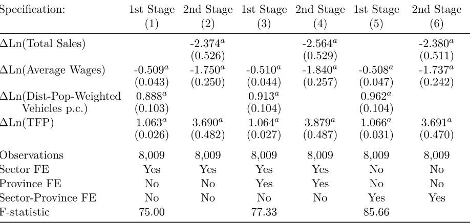
The two panels in Figure C.4 provide a graphical representation of the relationship between our baseline instrument (i.e., the municipality-specific distance- and population-weighted average of the stock of vehicles per capita in every other municipality, with weights built using the estimates in column 1 of Table1) and the boom-to-bust change in both the log of domestic sales (panel (a)) and exports (panel (b)). Panel (a) thus represents the first-stage relationship between the endogenous covariate and the instrument, while panel (b) represents the reduced-form relationship between the outcome variable of interest and the instrument.

C.5 Variation in the Instrument at the Municipal Level

(4)

Figure C.3: The Great Recession in Madrid and Barcelona: Variation Across Zip Codes

(a) Relative Change in Domestic Sales

(Madrid) (b) Relative Change in Cars per Capita(Madrid)

(c) Relative Change in Domestic Sales

(Barcelona) (d) Relative Change in Cars per Capita(Barcelona)

(5)

Figure C.4: First-Stage and Reduced-Form Relationships

-.3

-.2

-.1

0

.1

.2

Change in log Domestic Sales

-.2 0 .2 .4

Change in log Distance-Population Weighted Vehicles p.c.

(a) First-Stage Relationship

-1

-.5

0

.5

1

Change in log Exports

-.2 0 .2 .4

Change in log Distance-Population Weighted Vehicles p.c.

(b) Reduced-Form Relationship

Notes: Each dot represents the average change in log domestic sales (panel a) and in log exports (panel b) for a given value of the change in our baseline instrument (i.e., the municipality-specific distance- and population-weighted average of the stock of vehicles per capita in every other municipality, with weights built using the estimates in column 1 of Table 1). Observations are grouped into 30 equal-sized intervals of the horizontal axis, with the exception of cases where a bin contains five or less observations (which are grouped together to reduce the influence of outliers). The darkness of the markers is proportional to the number of observations in each bin. The regression lines depicted are estimated using the same number of observations (N=8,009) as in the regressions of Table3, without including any controls or fixed effects.

Figure C.5: Within-Province Variation in the Baseline Instrument

0

200

400

600

800

F

re

q

u

e

n

cy

-6 -4 -2 0 2 4 6

Baseline IV Net of Province Means (Standard deviations)

(6)

D Additional Macroeconomic Evidence

D.1 Basic Motivating Facts for Spain and Other Countries

In this Appendix, we present figures analogous to Figure 1 for a wider set of EMU-12 countries, and explore how the findings would change if we exclude the export of vehicles from the export series.

Each of the figures in this Appendix contain two panels. Panel (a) plots, relative to the total for all EMU-12 countries, a country’s share of extra-EMU-12 exports of goods and the corresponding country’s share of nominal GDP. Panel (b) includes an analogous plot but excludes from the export data all HS6 industries included the HS2 category “Vehicles; other than railway or tramway rolling stock, and parts and accessories thereof” (HS2 code 87). The data on exports is from UN Comtrade, and the nominal GDP data is from the AMECO database. We present these figures for eight countries: Spain, Portugal, Greece, Ireland, Italy, Germany, France, and the Netherlands.

Several observations are in order. First, the patterns in Spain, Portugal and Greece are quite similar, with the steep decline in the relative GDP of these countries around the crisis being accompanied by a significant increase in their export share to non-EMU-12 countries. Second, we observe in Germany and France the mirror image of the patterns observed in Southern Europe, with an increase in the relative GDP of those countries and a decline in their export share around the crisis. Third, the cases of the Netherlands and Italy are distinct in that one observes a fairly stable positive correlation between the relative GDP and relative export shares of those countries. Finally, excluding the motor vehicle industry from the relative export series has a very minor effect on these figures. This means, in particular, that the Spanish export miracle has little to do with dynamics in that sector.

We do not interpret these figures as providing compelling evidence that the vent-for-surplus mechanism was important for a variety of countries, but rather we invoke them to sustain the claim that the macroeconomic facts that motivate our study appear to be relevant for other countries. Whether the vent-for-surplus mechanism was key for other countries is left as an open question for future research.

Figure D.1: Share of Extra-Eurozone Exports and GDP in the EMU-12 Countries: Spain (a) All Industries

9 10 11 12 Sh a re o f N o mi n a l G D P (% ) 5 5.5 6 6.5 Sh a re o f Ext ra -EU R O 1 2 Exp o rt s (% )

2000 2002 2004 2006 2008 2010 2012 2014

Year

Share of Extra-EURO12 Exports Share of Nominal GDP

(b) Excluding Motor Vehicle Industry

9 10 11 12 Sh a re o f N o mi n a l G D P (% ) 4.5 5 5.5 6 6.5 Sh a re o f Ext ra -EU R O 1 2 Exp o rt s (% )

2000 2002 2004 2006 2008 2010 2012 2014

Year

(7)

Figure D.2: Share of Extra-Eurozone Exports and GDP in the EMU-12 Countries: Portugal (a) All Industries

1.75 1.8 1.85 1.9 1.95 Sh a re o f N o mi n a l G D P (% ) .8 .85 .9 .95 1 1.05 Sh a re o f Ext ra -EU R O 1 2 Exp o rt s (% )

2000 2002 2004 2006 2008 2010 2012 2014 Year

1.75 1.8 1.85 1.9 1.95 Sh a re o f N o mi n a l G D P (% ) .85 .9 .95 1 1.05 1.1 Sh a re o f Ext ra -EU R O 1 2 Exp o rt s (% )

2000 2002 2004 2006 2008 2010 2012 2014 Year

Figure D.3: Share of Extra-Eurozone Exports and GDP in the EMU-12 Countries: Greece (a) All Industries

1.8 2 2.2 2.4 2.6 Sh a re o f N o mi n a l G D P (% ) .6 .8 1 1.2 Sh a re o f Ext ra -EU R O 1 2 Exp o rt s (% )

2000 2002 2004 2006 2008 2010 2012 2014 Year

1.8 2 2.2 2.4 2.6 Sh a re o f N o mi n a l G D P (% ) .8 .9 1 1.1 1.2 1.3 Sh a re o f Ext ra -EU R O 1 2 Exp o rt s (% )

2000 2002 2004 2006 2008 2010 2012 2014 Year

Figure D.4: Share of Extra-Eurozone Exports and GDP in the EMU-12 Countries: Ireland (a) All Industries

1.6 1.8 2 2.2 Sh a re o f N o mi n a l G D P (% ) 3 4 5 6 Sh a re o f Ext ra -EU R O 1 2 Exp o rt s (% )

2000 2002 2004 2006 2008 2010 2012 2014

Year

1.6 1.8 2 2.2 Sh a re o f N o mi n a l G D P (% ) 3 4 5 6 7 Sh a re o f Ext ra -EU R O 1 2 Exp o rt s (% )

2000 2002 2004 2006 2008 2010 2012 2014

Year

(8)

Figure D.5: Share of Extra-Eurozone Exports and GDP in the EMU-12 Countries: Italy (a) All Industries

16.5 17 17.5 18 Sh a re o f N o mi n a l G D P (% ) 12.5 13 13.5 14 14.5 Sh a re o f Ext ra -EU R O 1 2 Exp o rt s (% )

2000 2002 2004 2006 2008 2010 2012 2014

Year

16.5 17 17.5 18 Sh a re o f N o mi n a l G D P (% ) 13.5 14 14.5 15 15.5 Sh a re o f Ext ra -EU R O 1 2 Exp o rt s (% )

2000 2002 2004 2006 2008 2010 2012 2014

Year

Figure D.6: Share of Extra-Eurozone Exports and GDP in the EMU-12 Countries: Germany (a) All Industries

27 28 29 30 31 Sh a re o f N o mi n a l G D P (% ) 35 36 37 38 39 Sh a re o f Ext ra -EU R O 1 2 Exp o rt s (% )

2000 2002 2004 2006 2008 2010 2012 2014

Year

27 28 29 30 31 Sh a re o f N o mi n a l G D P (% ) 32 33 34 35 36 Sh a re o f Ext ra -EU R O 1 2 Exp o rt s (% )

2000 2002 2004 2006 2008 2010 2012 2014

Year

Figure D.7: Share of Extra-Eurozone Exports and GDP in the EMU-12 Countries: France (a) All Industries

21 21.2 21.4 21.6 21.8 Sh a re o f N o mi n a l G D P (% ) 12 13 14 15 16 Sh a re o f Ext ra -EU R O 1 2 Exp o rt s (% )

2000 2002 2004 2006 2008 2010 2012 2014

Year

21 21.2 21.4 21.6 21.8 Sh a re o f N o mi n a l G D P (% ) 13 14 15 16 17 Sh a re o f Ext ra -EU R O 1 2 Exp o rt s (% )

2000 2002 2004 2006 2008 2010 2012 2014

Year

(9)

Figure D.8: Share of Extra-Eurozone Exports and GDP in the EMU-12 Countries: Netherlands (a) All Industries

6.5 6.6 6.7 6.8 6.9 Sh a re o f N o mi n a l G D P (% ) 7 8 9 10 Sh a re o f Ext ra -EU R O 1 2 Exp o rt s (% )

2000 2002 2004 2006 2008 2010 2012 2014 Year

6.5 6.6 6.7 6.8 6.9 Sh a re o f N o mi n a l G D P (% ) 8 9 10 11 Sh a re o f Ext ra -EU R O 1 2 Exp o rt s (% )

2000 2002 2004 2006 2008 2010 2012 2014 Year

D.2 Behavior of the Exports-to-Sales Ratio in Spain

The dynamics of the exports-to-sales ratio for firms in our baseline sample of continuing exporters is consistent with the macro evidence, as shown in FigureD.9 below. The exports-to-sales ratio is stable around 26% in the boom period (2002-2008) and increases sharply to about 30% during the recession, especially between 2009 and 2012.

Figure D.9: Exports-to-Sales Ratio for Continuing Exporters (Baseline Sample)

20 22 24 26 28 30 32 Exp o rt s/ Sa le s R a ti o (i n % )

2002 2004 2006 2008 2010 2012

Year

(10)

Figure D.10: Exports-to-Sales Ratio by Sector (a) Negative Growth Sectors

0

10

20

30

40

50

60

70

Exp

ort

s/

Sa

le

s

R

at

io

2002 2004 2006 2008 2010 2012

Year

Beverages Textiles

Leather&Shoes Paper

Printing Chemicals

Other

(b) Low Growth Sectors

0

10

20

30

40

50

60

70

Exp

ort

s/

Sa

le

s

R

at

io

2002 2004 2006 2008 2010 2012

Year

Food Clothing

Wood Pharmaceutical

Fabr. Metals Computer&Electron.

(c) High Growth Sectors

0

10

20

30

40

50

60

70

Exp

ort

s/

Sa

le

s

R

at

io

2002 2004 2006 2008 2010 2012

Year

Rubber&Plastic Minerals

Electrical Equip. Basic Metals

Mach. & Equip. Other Transp. Equip.

(11)

but below 2%) or high (above 2%) growth in their exports-to-sales ratio between the boom and bust periods. The annual patterns are shown in Figure D.10. The ratio is flat or declining in traditional sectors like beverages, textiles, paper, leather and shoes, and also for printing and chemicals. It features moderate growth in sectors like food, clothing, wood, fabricated metals, pharmaceutical products and computers & electronics. Finally, the exports-to-sales ratio increases strongly mostly in sectors such as electrical equipment, machinery & equipment (including repairs), other transportation equipment (different from vehicles), furniture, rubber & plastics, basic metals, and nonmetallic minerals.

D.3 Behavior of Export Prices

In this section, we describe the time series of the unit values of Spanish exports relative to that of the eleven countries (other than Spain) that belonged to the monetary union all throughout our sample period: Austria, Belgium, France, Finland, Germany, Greece, Ireland, Italy, Luxembourg, Netherlands and Portugal. With this aim, we collect data from U.N. Comtrade on the export unit values Pjdst for every one of these countries of origin j, every possible destination market d, every

HS6 product codes, and every yeartbetween2002and2013. Using this data, we estimate the year

fixed effectsλt and the sector- and destination-specific fixed effectsµds in the following regression:

ln(PSP dst/PEU dst) =λt+µds+εdst, (D.1)

wherePSP dstis Spain’s export unit value to destinationdin goodsand yeart,PEU dstis a weighted

average of the export unit valuesPjdstacross all eleven countries other than Spain belonging to the

European Monetary Union for all years between 2002 and 2006, andεdst is a regression residual.

We estimate the parameters of the regression in equation (D.1) under two alternative definitions of the average price PEU dst. First, we use an average price that uses weights that are fixed over

time:

PEU dst=

X

j6=SP

ωjds2000Pjdst, (D.2)

where ωjds2000 equals the ratio of exports of good s from country j to destination d in the year

2000 relative to the total exports of goodsfrom all eleven countries we have selected as comparison

group. Second, we use an average price that uses weights that vary over time:

PEU dst=

X

j6=SP

ωjdstPjdst, (D.3)

whereωjdst equals the ratio of exports of goods from countryj to destination din year trelative

to the total exports of goodsfrom all eleven countries we have selected as comparison group.

Figure D.11reports the OLS estimates ofλtin equation (D.1). These estimates are normalized

so that λ2007 = 0. Panel (a) reports the corresponding estimates for the case in which PEU dst is

computed using the expression in equation (D.2); Panel (b) reports similar estimates when the formula in equation (D.3) is used to computePEU dst. Both panels illustrate that the unit values of

(12)

Figure D.11: Export Unit Values of Spain Relative to Other Euro-area Countries (a) With Constant Weights

-.15

-.1

-.05

0

.05

Year FE

2002 2003 2004 2005 2006 2007 2008 2009 2010 2011 2012 2013

Year

(b) With Time-Varying Weights

-.15

-.1

-.05

0

Year FE

2002 2003 2004 2005 2006 2007 2008 2009 2010 2011 2012 2013

Year

A comparison of Figure D.11with Figure1 shows that the evolution of relative Spanish export unit values is positively correlated with the evolution of relative Spanish GDP and negatively correlated with the evolution of relative Spanish exports. These facts are consistent with our model. Because of an increasing marginal cost curve, prices are higher when total production is higher, and vice versa. They are also consistent with the relative reduction in export unit values explaining the extraordinary growth in total exports that took place in Spain (relative to other Euro countries) during the bust period.

Figure D.12: Export Unit Values of Spain Relative to Germany and France (a) Relative to Germany

-.1

-.05

0

Year FE

2002 2003 2004 2005 2006 2007 2008 2009 2010 2011 2012 2013

Year

(b) Relative to France

-.25

-.2

-.15

-.1

-.05

0

Year FE

2002 2003 2004 2005 2006 2007 2008 2009 2010 2011 2012 2013

Year

(13)

D.4 Home Bias in Firms’ Tax Records versus the C-Intereg Dataset

In this Appendix, we briefly compare some aggregate statistics on firms’ within-Spain sales from our tax records and from the C-Intereg dataset. We will then provide a sectoral decomposition of the home bias in the latter dataset.

In our 2006 aggregate data on municipality-to-municipality flows for firms in the manufacturing sector (which excludes sales of businesses in the auto industry), the average share of sales in which the origin and destination are the same municipality is 8.75%. This share increases to 25.4% when we consider sales within the seller’s own province and to 34.9% for sales in the seller’s region (or “Autonomous Community”, to use the legal term in Spain).1

C-Intereg is a micro-database constructed from a random sample of shipments by road within Spain during the period 2003-2007. Although we do not have access to this micro-database, we have obtained province-to-province shipments from that database.2 _{An advantage of the C-Intereg}

dataset is that it is representative at the sectoral level and, thus, allows to compute valid estimates of sector-specific own-province shares of shipments. As FigureD.13demonstrates, the own-province sales shares ranges from a low 18% in Transport Equipment (an industry we exclude from our anal-ysis) to a high of 43% for Nonmetallic Minerals. The overall provincial home bias in manufacturing in the C-Intereg dataset is 28%, which is quite close the 25.4% we computed in our dataset based on tax records.

Figure D.13: Province-Level Home Bias in Spanish Manufacturing

Food & Beverages

Textiles & Clothing

Leather & Footwear

Wood Products

Paper, Print & Arts

Chemicals

Rubber & Plastic

Nonmetallic Minerals

Basic & Fabricated Metals

Machinery & Equipment

Electrical Equipment

Transport Equipment

Other Manufacturing

0 .1 .2 .3 .4 .5

Proportion of Own-Province Sales

1_{In Spain, there are 8,018 municipalities, which are part of 50 provinces, and 17 autonomous communities. There} are also two autonomous cities, Ceuta and Melilla.

(14)

E Econometric Biases

E.1 Biases Due to Measurement Error in Exports and Total Sales

We discuss here the implications of measurement error in total sales and exports when a firm’s domestic sales are computed by subtracting its exports from its total sales (see also Berman et al., 2015).

Suppose that one does not observeRid directly, but instead measures it asRi−Rix, where Ri

and Rix denote the total sales and aggregate exports of firm i, respectively. Assume furthermore

that both∆ lnRi and ∆ lnRix are measured with error, so that

∆ lnRi = ∆ ln ˘Ri+$i and ∆ lnRix = ∆ ln ˘Rix+$ix,

where_Ri˘ _and _Rix˘ _{denote the true values of total sales and exports. Note then that}

∆ lnRid= ∆ lnRi−∆ lnRix= ∆ ln ˘Ri−∆ ln ˘Rix+$i−$ix,

Following the same steps as in the main text, we reach an estimating equation that differs from that in equation (6) only in that the regression residual now includes the measurement error in exports; i.e.,

εix = (σ−1) [uξ_ix+uϕ_i −uω_i] +$ix.

Similarly, we reach an expression analogous to that in equation (8) except that the regression residual now depends on the measurement error in total sales and exports; i.e.,

εid= (σ−1) [uξ_id+uiϕ−uωi] +$iT −$ix.

It then follows that the probability limit of the OLS estimator

plim( ˆβOLS) = cov(∆ lnRix,∆ lnRid)

var(∆ lnR_id)

can we written as

plim( ˆβOLS) =

cov(uξ_ix+uϕ_i −u_iω+ _σ₋1₁$ix, uξid+u

ϕ

i −uωi +σ−11($iT −$ix))

var(uξ_id+uϕ_i −u_iω+_σ₋1₁($iT−$ix)) .

This expression is analogous to that in equation (11) but it highlights the potential for additional sources of bias related to the covariance between the measurement error terms$ix and$iT−$ix.

The sign of this bias depends on the correlation between the measurement errors in total sales and in exports. If these variables are constructed from different sources (e.g., total sales are obtained from census data, while exports are drawn from customs data) it seems plausible that these measurement errors will be uncorrelated with each other; in this case, the impact of measurement errors in total sales and exports on the bias in the OLS estimate _βˆ_OLS _{will be negative. Nevertheless, if}

(15)

Consider next an IV estimator of β, where ∆ lnRid is instrumented with a variable Zid. The

probability limit of this IV estimator is

plim( ˆβIV) =

cov(uξ_ix+uϕ_i −uω_i +_σ₋1₁$ix,Zid)

cov(uξ_id+uϕ_i −uω

i + σ−11($iT −$ix),Zid)

.

This expression illustrates thatplim( ˆβIV) = 0as long as the instrumentZidverifies three conditions:

(a) it is correlated with the change in domestic sales of firmiafter partialling out sector fixed effects

and the observable determinants of the firm’s marginal cost that we include in our regression specification; (b) it is mean independent of the change in firm-specific unobserved productivity,uϕ_i,

factor costs,uω

i, and export demandu ξ

ix; and (c) it is mean independent of the measurement error

in exports$ix.

E.2 Analysis of the Model with Multiple Domestic and Foreign Markets

The benchmark model described in section 7accounts for one aggregate domestic market and one aggregate foreign market. We generalize here this model to incorporate multiple domestic markets and multiple foreign markets. One can interpret the multiple domestic markets as capturing Spanish municipalities, and the multiple foreign markets as capturing foreign countries.

We exploit the model described here to study how the existence of multiple domestic and foreign markets impacts possible biases affecting the OLS and several IV estimators of the elasticity of a firm’s total exports with respect to demand-driven changes in the firm’s total sales (i.e., sum of total exports and aggregate domestic sales). Specifically, we present simulation results that are informative about the sign of these biases and their quantitative importance.

E.2.1 Model: Description and Solution Algorithm

Notation. We use ito index firms, j to index markets, and t to index time periods. We useJit to

denote the set of markets to which firmisells at period t. Similarly, we useJidt andJixt to denote

the set of domestic and foreign markets, respectively, to which a firm exports at period t.

Demand function. We assume that the demand in any marketjat periodtfor the variety produced

by firmiis

Qijt=

P_ijt−σ

P_jt1−σEjtξ

σ−1

ijt . (E.1)

Rearranging terms, we can write the optimal pricePijt as

Pijt=Q−

1 σ

ijt P

σ−1 σ

jt E

1 σ

jtξ

σ−1 σ

ijt . (E.2)

Variable costs. Firm i’s total variable cost of producingQijt units in each market j∈Jit is

1

ϕitωit

1

λ+ 1(Qit)

λ+1 with _Q

it≡

X

j∈Jit

(16)

The marginal cost to firmiin periodt of sellingQijt in market j is thus

ωitτij

ϕit

(X

j∈Jit

τijQijt)λ. (E.3)

Fixed costs. We assume that a firmihas to pay fixed costsFijtto sell a positive amount in market j at periodt.

Market structure. We assume that firms are monopolistically competitive and, thus, their optimal price in any marketjat periodtis equal to a constant markupσ/(σ−1)over the marginal cost of

selling in market j att. Therefore, using the marginal cost expression in equation (E.3), the price

set by firm iin market j in periodtis:

Pijt=

σ

σ−1

ωitτij

ϕit

(X

j∈Jit

τijQijt)λ. (E.4)

Market-specific sales. The optimal quantity sold by firmiin each marketjbelonging to the setJit

is determined as the outcome of the following optimization problem

max

Qijt∈Jit

n Q

σ−1 σ

ijt P

σ−1 σ

jt E

1 σ

jtξ

σ−1 σ

ijt −

1

ϕit

ωit 1

λ+ 1(

X

j∈Jit

τijQijt)λ+1

o .

The first-order condition corresponding to eachQijt∈Jit is

σ−1

σ Q

−1

σ

ijt P

σ−1 σ

jt E

1 σ

jtξ

σ−1 σ

ijt −

ωitτij

ϕit (

X

j∈Jit

τijQijt)λ = 0,

and, thus, the optimal quantity sold by firm iin marketj at periodt is

Qijt=Ejt

1

ξijt

1

Pjt

1−σ σ

σ−1

ωitτij

ϕit

−σ

(X

j∈Jit

τijQijt)−λσ. (E.5)

Combining equations (E.4) and (E.5), we can write the optimal revenue of firm i in market j at

periodtas

Rijt≡QijtPijt=Ejt

1

ξijt

τij

Pjt σ

σ−1

ωit

ϕit

−(σ−1)

(X

j∈Jit

τijQijt)−λ(σ−1). (E.6)

Furthermore, given that,

X

j∈Jit

τijQijt=

X

j∈Jit

τij

Rijt

Pijt

= X

j∈Jit

Rijt

σ−1

σ

ϕit

ωit

(X

j∈Jit

τijQijt)−λ

= σ−1

σ

ϕit

ωit(

X

j∈Jit

τijQijt)−λ X

j∈Jit

(17)

= σ−1 σ

ϕit

ωit(

X

j∈Jit

τijQijt)−λRit,

we can rewrite

(X

j∈Jit

τijQijt)1+λ = σ−1

σ ϕit ωit Rit and (X

j∈Jit

τijQijt)−λ(σ−1) =

σ−1

σ ϕit

ωit

Rit

−λ(σ−1)

1+λ

.

Plugging this expression in equation (E.6), we can further rewrite the optimal revenue of firmiin

marketj at periodtas

Rijt=Ejt

1

ξijt

τij

Pjt

σ

σ−1

ωit

ϕit

−(σ−1)σ−1

σ

ϕit

ωit

Rit

−λ(σ_1+λ−1)

=Ejt

σ

σ−1

ωit

ϕit

−σ−1

1+λ 1

ξijt

τij

Pjt

−(σ−1)

Rit

−λ(σ−1)

1+λ _, (E.7)

whereRit denotes the total sales of firmiat periodt.

Aggregate domestic sales and total exports. Thus, using the expression in equation (E.7), we can write aggregate domestic sales as

Ridt =

X

j∈Jidt

Rijt=

σ

σ−1

ωit

ϕit

−σ_1+λ−1

Rit

−λ(σ−1)

1+λ X

j∈Jidt

Ejt

1

ξijt

τij

Pjt

−(σ−1)

, (E.8)

total exports as

Rixt=

X

j∈Jixt

Rijt=

σ

σ−1

ωit

ϕit −σ_1+λ−1

Rit

−λ(σ_1+λ−1) X

j∈Jixt

Ejt

1

ξijt

τij

Pjt

−(σ−1)

, (E.9)

and total sales as

Rit=Ridt+Rixt=

σ

σ−1

ωit

ϕit

−σ−1

1+λ X

j∈Jit

Ejt

1

ξijt

τij

Pjt

−(σ−1)_1+λσ1+λ

. (E.10)

Market participation. The optimal variable profits that a firmiwill make in a market jand yeart

upon entry is given by

πijt= 1

σRijt. (E.11)

(18)

total profits that a firm iwill make in any given market j and yeart upon entry is given by

Πijt=πijt−Fijt. (E.12)

Consequently, the total profits of a firm iselling in a set of markets Jit at periodtis

ΠJit

it =

X

j∈Jit

Πijt. (E.13)

Firms are assumed to select the set of markets they sell to in order to maximize their total profits; thus, the optimal set of markets a firm sells to at period tis

Jit= arg max

J

ΠJ_it, (E.14)

whereJ denotes a generic set of possible markets to which a firm may sell to.

Solution algorithm. The empirically relevant objects entering our estimating equations are the aggregate domestic sales, Ridt, total exports, Rixt, and total sales Rit. For every possible firm i

and period t, we implement the following procedure in order to computeRidt,Rixt and Rit.

Our procedure requires looping over every every possible set J of markets to which firm imay

sell to in period t. For eachJ, we implement the following steps. First, we use equation (E.10) to

compute Rit. Second, we use equations (E.7), (E.11) and (E.12) to compute Rijt, πijt, and Πijt,

respectively, for every marketj belonging to the setJ. Third, we use equation (E.13) to compute ΠJ_it. Once we knowΠJ_it for every possible set of marketsJ to which firmimay sell to in periodt, we

use (E.14) to compute the optimal set of markets Jit in which firm isells at period t. Knowledge

of Jit implies knowledge of Jidt and Jixt. Once we knowJidt,Jixt, andJit, we use equations (E.8)

to (E.10) to computeRidt, Rixt and Rit. Our approach becomes computationally infeasible when

the number of destinations is large, but we will restrict our simulations to a relatively low number of destinations. As mentioned below, one could use iterative algorithms to scale up our exercise to a larger number of destinations.

E.2.2 Estimating Equations, Estimators and Endogeneity Problems

The parameter of interest in our empirical application is the elasticity of total exports with respect to total sales. To mimic the baseline boom-to-bust identification approach we follow in the main draft, we derive an estimating equation from the model described in AppendixE.2.1that compares the outcomes between two periods t= 0 and t= 1.

We use the notation ∆ ln(Xit) ≡ ln(Xi1)−ln(Xi0) for every possible variable X and firm i.

Then, from equation (E.9), we can write an estimating equation analogous to that in equation (16) in section 7.1as

∆ ln(Rixt) =−σ−1

1 +λ ∆ ln(ωit)−∆ ln(ϕit)

−λ(σ−1)

1 +λ ∆ ln(Rit) + ∆ν

x

it,

∆ν_itx = ∆ ln X

j∈Jixt

Ejt

1

ξijt

τij

Pjt

−(σ−1)

. (E.15)

(19)

this parameter, we treat all variables in this regression equation expect for ∆ν_itx as observed. We

treat the term ∆ν_itx as unobserved, as it depends on unobserved firm-, market- and year-specific

demand shocksξijtand unobserved market and year-specific price indices Pjt.3,4

In section E.2.3, we illustrate the properties of both the OLS estimator as well as of two instrumental variable (IV) estimators that use each a different instrument for∆ ln(Rit). These two

instruments are measures of the market potential of a firm i at period t in the domestic market.

Specifically, indexing each of the two instruments withk= 1,2, both instruments take the form

∆z_it,(k)d = ∆ ln X

j∈Jd

Ωij,(k)Ejt

1

ξijt

τij

Pjt

−(σ−1)

, (E.16)

whereJd denotes the set of all domestic markets, andΩij,(k) is the weight assigned to marketjfor

firm iaccording to instrumentk.

For the instrument ∆zd_it,(1), the weights are

Ω_ij,(1)≡τbα1

ij , for alli andj (E.17)

where, as a reminder,τij captures the trade costs from the municipality whereiis located to market j, and α1_b is the OLS estimate ofα1 in the estimating equation

ln(Rij1) =δj,1+α1ln(τij) +εij1, E[εij1|τij] = 0, (E.18)

where δj,1 denotes the destination-j and year-1 fixed effect. When estimating the parameter α1,

we use only information for those firms and destinations such thatj∈Jd andRij1 >0.

For instrument ∆z_it,(2)d , the weights are

Ω_ij,(2)≡Rij1/Rid1, (E.19)

or, equivalently, the share of the aggregate domestic sales of firm iat period1 that correspond to

the domestic market j.

In words, the two instrumental variables defined in equations (E.16) to (E.19) correspond to the log difference between periods t= 0and t= 1 in a weighted sum of firm- and market-specific

demand shifters. These two instruments differ only in the weights. The first one assigns a weight to each municipality j that is a function of the trade costs between the municipality of location of

firmiand municipalityj. The second one assigns a weight to each municipalityjthat is a function

of the share of aggregate domestic revenue of firmiobtained in municipality j at periodt= 1.

The two instrumental variables defined in equations (E.16) to (E.19) are very similar to those we use in our empirical application. Specifically, the instrument defined by equations (E.16), (E.17)

3_{In our empirical application (see section}_7.1_{), we allow the supply shifters}_{∆ ln(}_ω

it)and∆ ln(ϕit)to be imperfectly

observed. This does not affect qualitatively the properties of the OLS and IV estimators, as the lack of observability of the demand shifterξijt and price index Pjt causes possible estimators of the parameter λ(σ−1)/(1 +λ) to be

biased in a way similar to how they would be if the supply shifters were not perfectly controlled for.

4_{Although the expression in equation (}_E.15_{) results from aggregating a destination-specific gravity equation, the} issues that arise in the estimation of the parameter of interest are different from those discussed in Redding and Weinstein (2019). The reason is that neither the relevant regressor nor the parameter of interest (i.e., neither

∆ ln(Rit) nor λ(σ−1)/(1 +λ)) vary by export market. Thus, when aggregating across destinations, the relevant

(20)

and (E.18) is very similar to both our baseline instrument as well as to those instruments used to compute the estimates reported in columns 2 to 4 of Table7. The instrument defined in equations (E.16) and (E.19) corresponds to that used in column 5 of Table 7. The reason we use period

t= 1 information in the construction of the weights Ω_ij,(k) for both instrumental variables k = 1

and k = 2 is that, in our empirical application, we only observe data on firm-specific sales across

domestic markets (municipalities) for one year, and this year is within our sample period.

We expect both the OLS and the two IV estimators defined in equations (E.16) to (E.19) to be biased. The source of this bias is the dependency of the error term in the structural equation, denoted as ∆νx

it in equation (E.15), on the optimal set of export destinations of firmi in periodt, Jixt. As the marginal cost function in equation (E.3) is non-constant (i.eλ6= 0), any variable that

affects a firm’s sales in any of the domestic markets will affect the marginal cost at which this firm can sell in any foreign market and, thus, will affect the set of markets to which this firm decides to export. Thus, it is not possible to find an instrumental variable that is both relevant and valid. While this is true, we illustrate in Appendix E.2.3that, for the two instrumental variables defined in equations (E.16) to (E.19), the bias in the estimate of−λ(σ−1)/(1 +λ) is small for most values

of the structural parameters.

E.2.3 Properties of Estimators: Simulation Results

For each parameterization we consider, we simulate our model 500 times. For each simulation, we solve the model for two periods, t = 0 and t = 1, and 8,000 firms. In terms of the number of

domestic and foreign markets, we consider the following configurations: (a) five domestic markets and five export markets; (b) seven domestic markets and seven export markets. Extending the set of markets beyond fourteen is computationally demanding, as determining the optimal set of domestic and export markets in which a firmi sells in a periodt requires solving a combinatorial

discrete choice problem with substitutabilities and multiple sources of heterogeneity. Given that the profit function features decreasing differences in the extensive margin of exports, in principle we could have implemented the iterative algorithm in Arkolakis and Eckert (2017) to scale up our exercise, but our simulations results are not much affected by moving from 10 to 14 countries, so we have not pursued this approach here.

We set the elasticity of substitution to equal six (i.e., σ = 6) and the parameter determining

the slope of the marginal cost function with respect to total output to equal 0.904 (i.e.,λ= 0.904).

This implies that the elasticity of exports with respect to demand-driven changes in total sales is equal to−λ(σ−1)/(1 +λ) =−2.374, which coincides with the point estimate reported in column

3 of Table10.

We also impose the following distributional assumptions:

ln Ejt(Pjt)σ−1

= 0, (E.20a)

ln(ωit/ϕit)∼N(0,1), (E.20b)

ln (τij)−(σ−1)

∼N(0,1), (E.20c)

ln (ξijt)σ−1 ∼N(0, σ_ξ2), withσ2_ξ ={1,5}, (E.20d)

with ln(ωit/ϕit) independent across firms and years, ln (τij)−(σ−1) independent across firms and

(21)

we eliminate all randomness in the country- and year-specific shifter Ejt(Pjt)σ−1 because, as the

number of countries we can accommodate in our simulation is very small, the results would be entirely driven by the few random draws of this variable. In equation (E.20d), we denote the variance ofln (ξijt)σ−1

as

σ2_ξ; we present simulation results for two different values of the variance

parameterσ2

ξ,σ2ξ = 1 and σξ2= 5.

Concerning the fixed costs to firm i of selling in market j at period t, we impose that one of

the domestic markets has zero fixed costs and, for the remaining domestic markets, we impose the following distributional assumption

Fijt=f

(σ−1)(1+λ)

1+λσ

ijt with fijt ∼N(0, σf2) and σ2f ={1,5}, (E.21)

with _f˜_ijt _{is independent across firms, markets, and years. We present simulation results for two}

different values of the variance parameter σ2_f,σ_f2 = 1 and σ_f2 = 5.

Concerning the fixed costs of selling in export markets, we consider two different sets of as-sumptions. First, a case in which we treat foreign markets analogously to domestic markets; i.e., we impose that one foreign market has zero fixed costs and, for the remaining export markets, we impose the distributional assumption in equation (E.21). Second, a case in which we assume that fixed costs for all foreign markets follow the distributional assumption in equation (E.21); i.e., we do not restrict the fixed costs of any foreign market to equal zero. These two models differ in that only in the former will it be true that all firms have positive aggregate exports in every periodt; i.e., Rixt >0for alliandt. Conversely, when fixed costs do not equal zero for all foreign markets, there

are some firms that decide to not sell in any foreign market in some periodt; for these firms, it is

the case thatRixt = 0and, consequently, they are not used in the estimation of−λ(σ−1)/(1 +λ).5

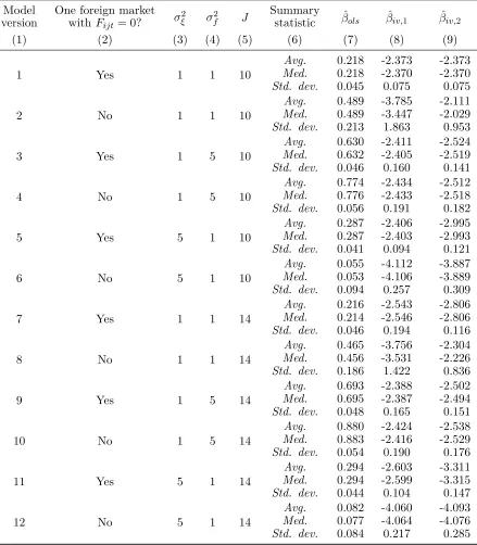
In Table E.1, we present simulation results for 12 different version of our model. Each version differs on whether fixed costs for one foreign market are set to zero (indicated in column 1), the value of σ2_ξ (indicated in column 2); the value ofσ_f2 (indicated in column 3); and the total number

of markets (indicated in column 4). In column 5, we indicate the average, median and standard deviation of the OLS estimates of the parameter −λ(σ −1)/(1 +λ) in the estimating equation

in equation (E.15). In column 6 and column 7, we present the same summary statistics for two instrumental variable estimates of−λ(σ−1)/(1+λ); the IV estimate whose distribution is described

in column 6 uses as instrument the variable defined in equations (E.16) and (E.17), the IV estimate whose distribution is described in column 7 uses as instrument the variable defined in equations (E.16) and (E.19).

We can extract several lessons from the results in Table E.1. First, the OLS estimator of the parameter of interest−λ(σ−1)/(1 +λ)is always biased positively; in fact, although the true value

of this parameter is -2.374, the OLS point estimate is always positive and the standard deviation of these OLS point estimates across the 500 simulations is relatively small. Second, for most data generating process considered in our analysis, both IV estimators yield similarly distributed point estimates; specifically, in both cases, the average and the median IV point estimates tend to be smaller than the true parameter value. Third, in models in which all firms export (i.e., whenever we set to zero the fixed costs of selling in one of the foreign markets), the downward bias affecting the two IV estimators considered in Table E.1 is very small; typically, the average and median point estimates are within one standard deviation of the true parameter value. Fourth, in models in which only a subset of all active firms export (i.e., models in which the fixed costs of selling

5_{For these firms, the dependent variable of interest}_{∆ ln(}_R

(22)

Table E.1: Simulation Results

Model One foreign market

σ_ξ2 σ2_f J Summary βôls βîv,1 βîv,2

version withFijt= 0? statistic

(1) (2) (3) (4) (5) (6) (7) (8) (9)

1 Yes 1 1 10 Med.Avg. 0.2180.218 -2.373-2.370 -2.373-2.370 Std. dev. 0.045 0.075 0.075

2 No 1 1 10 Med.Avg. 0.4890.489 -3.785-3.447 -2.111-2.029 Std. dev. 0.213 1.863 0.953

4 No 1 5 10 Med.Avg. 0.7740.776 -2.434-2.433 -2.512-2.518 Std. dev. 0.056 0.191 0.182

6 No 5 1 10 Med.Avg. 0.0550.053 -4.112-4.106 -3.887-3.889 Std. dev. 0.094 0.257 0.309

8 No 1 1 14 Med.Avg. 0.4650.456 -3.756-3.531 -2.304-2.226 Std. dev. 0.186 1.422 0.836

10 No 1 5 14 Med.Avg. 0.8800.883 -2.424-2.416 -2.538-2.529 Std. dev. 0.054 0.190 0.176

12 No 5 1 14 Med.Avg. 0.0820.077 -4.060-4.064 -4.093-4.076 Std. dev. 0.084 0.217 0.285 Note: For each of the models indicated in column 1, results are based on 500 simulations. Avg.,Med. and

Std. dev. denote the average, median, and standard deviation, respectively, of the different estimates of

−λ(σ−1)/(1 +λ). βˆols denotes the OLS estimate;βˆiv,1 denotes the IV estimate that uses the expression

defined in equations (E.16) and (E.17) as instrument;_βˆ_iv,2 _{denotes the IV estimate that uses the expression}

defined in equations (E.16) and (E.19) as instrument. The true value of the parameter is−λ(σ−1)/(1+λ) = −2.374. In column 2, we indicate whether fixed costs are set to zero for one of the foreign markets. In column

3, we indicate the value of the parameterσξ2; in column 4, we indicate the value of the parameter σ2f; in

(23)

to every foreign market follow the distribution in equation (E.21)), the downward bias affecting the two IV estimators can be quantitatively important, and this bias increases in the variance of the demand shock, σ2_ξ, and decreases in the variance of the fixed costs of selling to a market, σ_f2.

Fifth, for all parameterizations we consider, the distribution of the OLS estimator as well as the distributions of the two IV estimators vary very little as we change the number of countriesJ.

E.3 Biases in the Extensive Margin of Exports

We extend here the analysis in section 2 to the study of the effect of domestic demand shocks on the extensive margin of exports.

Given the CES demand function in equation (1) and the assumption that firms are monopolis-tically competitive in every market, firm iwill find it profitable to export at time tonly if export

revenueRixt exceeds a multipleσof the fixed cost of exportingFixt. We can thus express a dummy

taking value one if firm iexports at period t asdixt=1{lnRixt > σlnFixt}, where 1{A} denotes

an indicator function that takes value one if and only if the statement A is true. The

probabil-ity that firm i exports conditional on a vector Xix ≡ {Xixt}t that includes a set of period- and

sector-specific fixed effects and observed proxiesϕ∗_it and ω_it∗ for every periodt is

Pr(dixt = 1|Xix) =E[dixt|Xix] =E[1{lnRixt > σlnFixt}|Xix].

Focusing on a linear probability model, we further rewrite the probability of firm i exporting at

periodtas

Pr(dixt = 1|Xix) =E[lnRixt−σlnFixt|Xix].

Therefore, we can write the change in the probability of exporting between any two periodst and t−1 as a function of the changes in the log export revenues and log fixed export costs

Pr(dixt= 1|Xix)−Pr(dixt= 0|Xix) = ∆ Pr(Xix) =E[∆ lnRix−σ∆ lnFix|Xix]

where, from equation (6),

∆ lnRixt =γsx+ (σ−1)δϕ∆ ln(ϕ∗_it)−(σ−1)δω∆ ln(ω∗_it) +εix,

with the different terms in this expression defined as in section 2and, analogously

∆ lnFixt=φsx+φϕ∆ ln(ϕ∗_i) +φω∆ ln(ω∗_i) +uF_i .

Notice that we are being quite flexible, letting firm-level fixed export costs depend on firm-level productivity and factor costs, and on sector fixed effects.

With these expressions at hand, we can write the change in the probability of exporting, ex-panded to include log domestic sales as an additional covariate, as

∆ Pr(Xix) =E

(γsx−φsx) + (γ`x−φ`x) + [(σ−1)γϕ−σφϕ]∆ ln(ϕ∗i)

−[(σ−1)δω−σφω]∆ ln(ω∗_i) +β∆ lnRid+εix−σuF_i Xix

,

(24)

the following asymptotic properties of_βˆ_OLS _{can be derived:}

plim( ˆβOLS) = cov(u

ξ

ix+u

ϕ

i −uωi −σ−σ1uFi , u

ξ

id+u

ϕ

i −uωi)

var(uξ_id+uϕ_i −uω

i)

.

The only difference relative to equation (11) is the addition of the term−(σ/(σ−1))uF_i in the first

element of the covariance in the numerator. It is clear that, as in the intensive margin regressions, this covariance is likely to be positive, thus generating a positive value ofplim( ˆβOLS).

The probability limit of the IV estimator of β is given by

plim( ˆβIV) =

cov(uξ_ix+uϕ_i −u_iω−_σ₋σ₁uF_i ,Z_id)

cov(uξ_id+u_iϕ−uω_i,Zid)

. (E.22)

This expression will equal zero as long as the instrument Z_id verifies the following two conditions:

(a) it is correlated with the boom-to-bust change in domestic sales of firm i, after partialling out

firm fixed effects and the boom-to-bust difference in observable determinants of the firm’s marginal cost; and (b) it is mean independent of the boom-to-bust changes in unobserved productivity, uϕ_i,

factor costs,uω_i, export demand shocks,uξ_ix, and export fixed-cost shocks uF_i (this latter being the

only additional condition relative to our results for the intensive margin regressions). As in our discussion in section2, an instrument can only (generically) verify conditions (a) and (b) if its effect on domestic sales works exclusively through the domestic demand shock uξ_id.

It is straightforward to extend the above analysis to the case in which total sales and exports (but not the dummy variabledixtindicating whether firm iexports at periodt) are measured with

error and domestic sales are imputed by subtracting exports from total sales. Following the same steps as in AppendixE.1, we obtain

plim( ˆβIV) = cov(u

ξ

ix+u

ϕ

i −uωi −σσ−1uFi + σ−11$ix,Zid)

cov(uξ_id+uϕ_i −uω

i + σ−11($iT −$ix),Zid)

.

Given that the numerator in this expression coincides with that in equation (E.22), the presence of measurement error in total sales and exports does not affect the conditions that the instrument

Zid must satisfy so that the probability limit of the IV estimator equals zero. Thus, as long as the

conditions (a) and (b) above are satisfied,plim( ˆβIV) = 0independently of the relationship between

the instrument and the measurement errors in total sales and exports.

E.4 The Relevance of Confounding Export Demand Shocks

As formalized in section 2.1 (see discussion of equation (12)) and in section 7.1, a possible source of bias affecting our TSLS estimates of the elasticity of changes in firms’ exports with respect to changes in their domestic (or total) sales is the possible non-zero correlation between our instrument and the changes foreign demand affecting each firm. Testing whether this non-zero correlation is present in our empirical setting is complicated by the fact that firm-specific export-demand shocks are not directly observed in our data.

(25)

shocks are adequately controlled for by the sector-specific fixed effects we include in all our regression specifications, heterogeneity in foreign demand shocks due to reason (a) will not bias our TSLS estimates of the elasticity of firms’ exports with respect to their domestic (or total) sales. Here, we study whether our estimates may be biased due to the heterogeneity in the set of foreign countries that firms export to.

Specifically, we explore here whether the boom-to-bust changes in the number of vehicles per capita in a municipality is correlated with a municipality-specific aggregator of the boom-to-bust demand shocks experienced by different foreign countries.

To construct municipality- and period-specific measures of foreign demand shocks, we follow a four-step procedure. First, for each destination country to which Spain exported a positive amount in 2002, we collect 2002-2013 data from UN Comtrade on its aggregate imports by product, country of origin and year, with a “product” corresponding either to an HS-2, an HS-4 or an HS-6 digit product code. Second, we regress the logarithm of this product-, origin-, destination-, and year-specific import measure on origin- and year-year-specific fixed effects, destination- and year-year-specific fixed effects and product- and year-specific fixed effects. We interpret the estimates of the destination-and year-specific fixed effects as estimates of destination- destination-and year-specific demdestination-and shifters after controlling for sectoral shifters. Third, we compute municipality-specific weighted averages of these destination- and year-specific demand shifters, where the weight that each destination country takes for each municipality equals the share of the 2002 exports of that municipality to that destination country. Fourth, we compute municipality-specific measures for the boom and bust periods as the average of the 2002-2008 years and the 2009-2013 years, respectively.

In Table E.2, we present OLS estimates of the coefficients in regressions of the boom-to-bust log change in the measure of foreign demand shocks whose construction is described in the previous paragraph on the boom-to-bust log change in the number of vehicles per capita. Each observation in these regressions corresponds to a municipality, and we weight each municipality by the number of firms located in the corresponding municipality that have positive exports in the boom and bust periods. The results show that, even if we use a 10% significance level test, we cannot reject the null hypothesis that the boom-to-bust log change in our measure of municipality-specific foreign demand shocks is uncorrelated with the boom-to-bust log change in the number of vehicles per capita in the corresponding municipality.

Table E.2: Correlation of Local and Foreign Demand Shocks

Product Definition: HS-2 HS-4 HS-6

(1) (2) (3)

∆Ln(Vehicles p.c.) -2.841 -0.622 -0.188

(2.189) (0.469) (0.177) (2.340) (0.504) (0.191)

Obs. 1,103 1,103 1,103

Notes: a_{denotes significance at the 1% level;}b_{denotes significance at the}

5% level;c_{denotes significance at the 10% level. In parenthesis, we report}

(26)

F Estimation of Revenue Productivity

We present a step-by-step description of our baseline estimation approach in Appendix F.1. For an analogous description of the alternative estimation approach used to compute the estimates in columns 3 and 4 of Table9, see Bilir and Morales (2020). We summarize the production function estimates that both approaches yield in AppendixF.2.

F.1 Baseline Estimation Approach

We describe here the procedure we follow to estimate a proxy for firm- and year-specific performance or revenue productivity under the assumption that the production function is Leontief in materials. We describe first the assumptions that we impose on the production function, the demand function, market structure, and the stochastic process of revenue productivity or performance. Given these assumptions, we illustrate how we estimate the demand elasticity σ and all parameters of the

revenue function. Finally, we describe how we use these estimates to recover a proxy of the revenue productivity or performance for every firm and year.

Assumption on production function. We assume a production function that is a Leontief function of materials and a translog aggregator of labor and capital:

Qit= min{H(Kit, Lit;α), Mit)}ϕit, (F.1a)

H(Kit, Lit;α) = exp(h(kit, lit;α)), (F.1b)

h(kit, lit;α)≡αllit+αkkit+αlllit2 +αkkkit2 +αlklitkit, (F.1c)

withα= (αl, αk, αll, αkk, αlk). In equation (F.1a),Kitis effective units of capital,Litis the number

of production workers, Mit is a quantity index of materials use, andϕit denotes the Hicks-neutral

physical productivity. To simplify the notation, we use here lower-case Latin letters to denote the logarithm of the upper-case variable, e.g.,lit = ln(Lit). The production function in equation (F.1)

nests that introduced in Appendix A, which implicitly assumes that αll =αkk =αlk = 0. In our

estimation, we impose noa priori restriction on the values of the elements of the parameter vector αand, thus, our estimation framework does not take a stand on whether marginal production costs are constant (as assumed in section2) or increasing (as assumed in section7).

Consistently with the definition of ϕit as physical productivity, we assume that

E[ϕit|Jit] =ϕit, (F.2)

whereJ_it denotes the information set of firmiat the time at which the period-tpricing and input

decisions are taken. Therefore, the firm knows the value of its productivity ϕit when making the

period-tpricing and input decisions.

We assume that both materials and labor are fully flexible inputs, and that capital is dynamic and determined one period ahead. Consequently, bothMit andLitare a function ofJit, whileKit

is a function of J_it−1.

(27)

ξit is known to firms when determining their input and output decisions; i.e.,

E[ξit|Jit] =ξit. (F.3)

Assumptions on market structure. As described in section 2, we assume that firms are monop-olistically competitive in the output markets and that they take the prices of labor, materials and capital as given.

Derivation of the revenue function. Given the assumption that materials is a flexible input, equation (F.1a) implies that optimal materials usage satisfies

Mit =H(Kit, Lit;α).

Therefore, we can rewrite the production function in equation (F.1a) as

Qit=H(Kit, Lit;α)ϕit, (F.4)

where H(Kit, Lit;α) is defined as in equations (F.1b) and (F.1c). Given this expression and the

demand function in equation (1), we can write the revenue function of a firmi at periodt as

Rit=PitQit=P

σ−1 σ

st E

1 σ

stξ

σ−1 σ

it Q

σ−1 σ

it =µstH(Kit, Lit;β)ψit, (F.5)

where

κ≡(σ−1)/σ, (F.6a)

β≡κα, (F.6b)

ψit≡(ξitϕit)κ (F.6c)

µst ≡Pstκ(Est)1−κ. (F.6d)

The parameterκmeasures the inverse of the firm’s markup. While the parameter vectorαincludes the production function parameters, the vector β includes the revenue function parameters. The variable ψit captures the revenue productivity of the firm: the residual determinant of a firm’s

revenue after controlling for sector- and year-specific fixed effects and for the effect of capital and labor on the firm’s revenue. As illustrated in equation (F.6c), revenue productivity equals in our model the product of the Hicks-neutral productivityϕit and the demand shifterξitto the power of

the reciprocal of the firm’s markup. The sector-year fixed effects accounts for the price index and total expenditure in the corresponding sector-year pair.

Assumptions on stochastic process for revenue productivity. We assume that revenue produc-tivity follows a first-order autoregressive process, AR(1), with a state- and year-specific shifter:

ψit=γst+ρψit+ηit with E[ηit|Jit] = 0. (F.7)

This stochastic process for revenue productivity may arise under different stochastic process for physical productivity ϕit and the demand shifter ξit; e.g., both variables follow AR(1) process

(28)

persistence parameter ρ and the other one is independent over time.

Estimation of demand elasticity. In order to estimate the demand elasticity σ, we follow the

approach implemented, among others, in Das, Roberts and Tybout (2007) and Antràs et al. (2017). Given the assumption that all firms are monopolistically competitive in their output markets, it will be true that

Rit−C_itv = 1

σRit,

where C_itv denotes the total variable costs that firm i incurred at period t to obtain the sales

revenue Rit. This expression indicates that the firm’s total profits (gross of fixed costs) is equal

to the reciprocal of the demand elasticity of substitutionσ multiplied by the firm’s total revenues.

Given that the only variable inputs are materialsMitand laborLit, we can rewrite this relationship

as

Rit−PitmMit−ωitLit=

1

σRit,

where P_itm denotes the equilibrium materials’ price faced by firm i at period t, ωit denotes the

equilibrium salary and, thus, P_itmMit denotes total expenditure in materials’ purchases andωitLit

denotes total payments to labor. Rearranging terms, we obtain the following equality

σ−1

σ

Rit =PitmMit+ωitLit,

and, allowing for measurement error in sales revenue, Robs_it ≡Ritexp(εit), we obtain

ln

σ−1

σ

+robs_it −εit= ln(P_itmMit+ωitLit),

where, as indicated above, lower-case Latin letters denote the logarithm of the corresponding upper case variable and, thus, r_itobs ≡ln(Robs_it ). Imposing the assumption that E[εit] = 0, we identify σ

through the following moment condition

Ehln

σ−1

σ

+robs_it −ln(P_itmMit+ωitLit)

i

= 0. (F.8)

Estimation of labor elasticity parameters. Given equation (F.5), we can write the profit function of firmiin periodt as

Πit =µstH(Kit, Lit;β)ψit−ωitLit−PitmMit−PitkIit,

where ωit denotes the wage that firm ifaces at period t and, analogously, Pitm and Pitk denote the

materials and capital prices. Assuming that labor is a fully flexible input and that firms are both monopolistically competitive in output markets and take the price of all inputs as given, the first order condition of the profit function with respect to labor implies that

∂Πit

∂Lit

(29)

Reordering terms and taking logs on both sides of the equality, we obtain

ln(βl+ 2βlllit+βlkkit) = ln(ωitLit)−rit,

and, taking into account that revenues are measured with error, we can further rewrite

ln(βl+ 2βlllit+βlkkit) = ln(ωitLit)−robsit +εit.

Assuming that the measurement error in revenue is not only mean zero (as imposed to derive the moment condition in equation (F.8)) but mean independent of the firm’s labor and capital usage,

E[εit|lit, kit] = 0,

we can derive the following conditional moment:

E[robs_it −ln(ωitLit) + ln(βl+ 2βlllit+βlkkit)|lit, kit] = 0.

We derive unconditional moments from this equation and use a method of moments estimator to estimate (βl, βll, βlk). With the estimates ( ˆβl,βˆll,βˆlk) in hand, we recover an estimate of the

measurement error εit for each firmi, affiliatej, and period t:

ˆ

εit=r_itobs−ln(ωitLit) + log( ˆβl+ 2 ˆβlllit+ ˆβlkkit).

Combining the estimates of the parameters entering the elasticity of the firm’s revenues with re-spect to labor,( ˆβl,βˆll,βˆlk), and the estimate of the demand elasticity of substitution, we compute

estimates of the parameters(αl, αll, αlk); i.e.,

( ˆαl,αˆll,αˆlk) = ˆ σ ˆ

σ−1( ˆβl,βˆll,βˆlk).

Estimation of capital elasticity parameters. Using the estimates ( ˆβl,βˆll,βˆlk) and εitˆ we can

construct a corrected measure of revenues

b

rit≡rit−βˆllit−βˆlll2it−βˆlklitkit−εˆit,

and, given the expression for sales revenues in equation (F.5), it holds that

b

rit=βkkit+βkkk2it+ψit.

Given this expression and the stochastic process for the evolution of productivity in equation (F.7), it will be true that

b

rit=βkkit+βkkk2it+µψ(brijt−1−βkkijt−1−βkkk

2

ijt−1) +ζst+ηit, (F.9)

whereζst is an unobserved sector- and time-specific effect that accounts for the revenue shifterµst

(30)

J_it, the definition ofηit in equation (F.7) implies that

E[ηit|kit,rbijt−1,{dst}s,t] = 0,

where {dst}s,t denotes a full set of sector- and time-specific dummy variables. Therefore, we can

derive the following conditional moment equality

E[_brit−βkkit−βkkkit2 −ρ(brijt−1−βkkijt−1−βkkk 2

ijt−1)−ζst|kit,brijt−1,{dst}s,t] = 0

We derive unconditional moments from this equation and use a method of moments estimator to estimate(βk, βkk, ρ). When estimating these parameters, we use the Frisch-Waugh-Lovell theorem

to control for the full set of sector- and time-specific fixed effects{ζst}s,t. Combining the estimates

of the parameters(βk, βkk), and the estimate of the demand elasticity of substitutionσ, we compute

estimates of the parameters(αk, αkk); i.e.,

( ˆαk,αˆkk) = ˆ σ ˆ

σ−1( ˆβk,βˆkk).

Estimation of productivity. We can also use the estimates of the parameters(βk, βkk) and the

constructed random variablebrit to build an estimate of the revenue productivity ψit for every firm

and time period

b

ψit=brit−βˆkkit−βˆkkk

2

it.

F.2 Production Function Estimates

We summarize here the production function and productivity estimates that we obtain both when we assume a production function that is Leontief in materials (see AppendixF.1for the correspond-ing estimation approach) and when we assume instead a production function that is Cobb-Douglas in materials (see Bilir and Morales, 2020, for the corresponding estimation approach). No matter which of these two production functions we assume, we estimate the corresponding production function parameters and demand parameters separately for the boom and bust periods and for each of the twenty-four 2-digit NACE sectors in which the manufacturing firms in our dataset are classified. For both the boom and the bust periods, we report here the simple average across all sectors of the estimated labor and capital elasticities, of the estimated persistence parameters ρ

and of the demand elasticity σ.

Under the assumption that the production function is Leontief in materials, we obtain the following estimates. In the boom period, the average elasticities of revenue with respect to labor and capital are 0.23 and 0.19, respectively; the average annual autocorrelation in performance is 0.97; and the average demand elasticity is 3.55. In the bust period, the average elasticities of revenue with respect to labor and capital are 0.26 and 0.18, respectively; the average annual autocorrelation in performance is 0.98; and the average demand elasticity is 3.37.

(31)

autocorrelation in performance is 0.78; and the average demand elasticity is 3.05.

Notice that both estimation approaches yield estimates of the demand elasticity σ that are

a bit low relative to those that, using identification strategies different from ours, are typically obtained in the international trade literature (see Head and Mayer, 2014, for a review). One possible explanation for this mismatch between our estimates and those in the international trade literature is the fact that we cannot observe firms’ expenditure in energy; this may imply that our measure of the variable production costs underestimates the firms’ total expenditure in variable inputs and, thus, that our estimates of σ are downward biased. These estimates of σ do not, however, impact

any of the estimates presented in the main draft. More specifically, the only exercise that we perform in the paper and that relies on the estimated value of σ is the quantification in section

7.2. However, as indicated in that section, our baseline quantification calibrates the value of σ to

a central value among the estimates computed in the international trade literature; i.e., σ= 5.

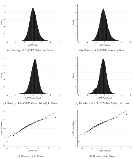
Panels (a) and (b) in Figure F.1show, respectively, that the marginal distribution in the boom and bust periods of the (log) TFP estimates computed following the procedure in sectionF.1. These two marginal distributions are symmetric around zero and close to normally distributed, reflecting that the distribution of the TFP estimates is close to log-normally distributed. Panels (c) and (d) show analogous marginal distributions for (log) TFP estimates computed following the procedure in Bilir and Morales (2020). While the distributions in panels (a) and (b) are similar to each other, that in panel (d) is clearly different from that in panel (c) in that the fraction of firms in the lower tail of the distribution is significantly larger. Thus, our value added-based TFP estimates show that the fraction of firms with relatively lower TFP increased in the bust period relative to the boom.

(32)

Figure F.1: Productivity Estimates

.1

.2

.3

.4

.5

Density

-6 -4 -2 0 2 4 6

Ln(TFP Sales)

(a) Density of Ln(TFP Sales) in Boom

.1

.2

.3

.4

.5

Density

-6 -4 -2 0 2 4 6

Ln(TFP Sales)

(b) Density of Ln(TFP Sales) in Bust

.1

.2

.3

.4

.5

Density

-6 -4 -2 0 2 4 6

Ln(TFP Value Added)

(c) Density of Ln(TFP Value Added) in Boom

.1

.2

.3

.4

.5

Density

-6 -4 -2 0 2 4 6

Ln(TFP Value Added)

(d) Density of Ln(TFP Value Added) in Bust

-2

-1

0

1

2

Ln(TFP Value Added)

-2 -1 0 1 2 3

Ln(TFP Sales)

(e) Binscatter in Boom

-3

-2

-1

0

1

Ln(TFP Value Added)

-2 -1 0 1 2 3

Ln(TFP Sales)

(f) Binscatter in Bust