CU Scholar
Computer Science Graduate Theses & Dissertations
Computer Science
Spring 1-1-2012
Face Detection Using Single Cascade of
Customized Features Discriminators
Ayman Omar Hammuda
Follow this and additional works at:
http://scholar.colorado.edu/csci_gradetds
Part of the
Artificial Intelligence and Robotics Commons
This Thesis is brought to you for free and open access by Computer Science at CU Scholar. It has been accepted for inclusion in Computer Science Graduate Theses & Dissertations by an authorized administrator of CU Scholar. For more information, please [email protected].
Recommended Citation
Hammuda, Ayman Omar, "Face Detection Using Single Cascade of Customized Features Discriminators" (2012).Computer Science Graduate Theses & Dissertations.Paper 51.
CUSTOMIZED FEATURES DISCRIMINATORS by
AYMAN OMAR HAMMUDA B.S., University of Tripol, Libya, 1995
A thesis submitted to the Faculty of the Graduate School of the University of Colorado in partial fulllment
of the requirements for the degree of Master of Science
Department of Computer Science 2012
DISCRIMINATORS
written by AYMAN OMAR HAMMUDA
has been approved for the Department of Computer Science
Assistant Prof. Nikolaus J. Correll
Associate Prof. Kenneth M. Anderson
Distinguished Prof. Andrzej Ehrenfeucht
Assistant Prof. Tom Yeh
Date
The nal copy of this thesis has been examined by the signatories, and we nd that both the content and the form meet acceptable presentation standards of scholarly work in the above
FACE DETECTION USING SINGLE CASCADE OF CUSTOMIZED FEATURES DISCRIMI-NATORS
Thesis directed by Prof. Assistant Prof. Nikolaus J. Correll
Face detection has become an important and helpful tool for camera and video processing. Useful human-computer interaction (HCI) applications such as drivers assistant system that prevents accidents and saves pedestrian lives when drivers attention is absent, needs a head pose estimator. A head pose estimator cannot function without face detector.
There has been a considerable amount of literature to address the problem. The most signif-icant results obtained on uptight frontal face detection which is a sub-problem of a larger problem of face detection. There are other types of sub-problems that has been studied with least signicant advancements that the upright frontal face detection had accomplished. The problem of multi-pose detection is still under study and it remains hard.
A solution to this large scale of the problem (multi-pose face detection) is critical in head pose accuracy. This thesis suggests a multi-pose face detection algorithm for uncontrolled environments. The detector is designed to be used in building head pose estimator for a human-computer inter-action application. The observed design of the detector has to implement a cascade of classiers. Each classier has to address at least one certain area of the problem. The design have to maintain speed and an acceptable detection rate.
These requirements can be satised by constructing the cascade to implement fast and simple classiers at rst stages of the cascade. A novel use of the integral image as a fast lter was invented to be placed at the start of the detection process. Included in the cascade, classiers that are trained on special designed features aimed to solve part of the problem. One special unique classier is a data mining based classier that uses a modied version of the Maximal Frequent Itemset Algorithm (MAFIA) [2] for feature extraction.
Special features classiers use the extracted facial features information extracted from a new knowledge-based classier/lter that was created with the capacity to locate to an acceptable ac-curacy the location of eyes, mouth and nose using a suite of approaches including discreet local minima and geometric measures. The extracted facial features were used to estimate head pose and extract classier features accordingly to enhance detection rates.
A cascade of classiers based on fast and simple contrast features was used to rene and speed up the detection process. To further improve speed some components were parallelized. As an attempt to overcome some of the fundamental challenges of face detection, lighting correction and noise reduction were implemented based on the information extracted from images.
Results are reported on the FDDB [12] benchmark showed 5.22% detection rate with 2000 false positives while OpenCV implementation of Viola-Jones [19] face detector showed 65.92 detection rate with 2010 false positives. This comparison is awed; because Viola-Jones is an upright face detector and even though FDDB [12] includes a number on non-frontal faces and proles the majority of the faces are frontal. The two solutions address two dierent problems that reect large dierences in diculty.
A standard benchmark testset and evaluation system as FDDB [12] benchmark and com-parable results from the same class of the problem at the time of writing this document was not available. The key points to building good face detector in general are; (1) resolving speed issues using fast techniques (e.g integral image) at the start of the cascade and a powerful design, (2) using a huge number of dierent strong and weak features, and (3) eliminating variations (i.e pose , noise and lighting variations). The algorithm was also tested on MIT+CMU upfront faces testset and reported 43.56% detection rate with 504 false positives.
To my beloved father Prof. Omar S. Hammuda, who raised me on the love of science and learning. He is also a University of Colorado at Boulder alumni for both his M.S. and Ph.D. Without his support I was not able to enroll in the same university that we both love and adore. Thank you father!
Acknowledgements
I am very grateful to the community of the University of Colorado at Boulder that gave me the opportunity to study at this great school. Special thanks to my former thesis asvisor Prof. Jane Mulligan to her eorts and contribution to this work. She was the rst professor that taught me in this school and introduced me to the eld of computer vision. Special thanks to Prof. Nikolaus J. Correll for his great support and for his acceptance to take the responsibility to advise me at the nal stage. Thanks to my academic asvisor and Prof. Kenneth M. Anderson who guided me thoughout the program and for accepting to be a member of the defense committee. Thanks to my professor the Distinguished Prof. Andrzej Ehrenfeucht for every advice and every letter I learned from him. Spacial thanks to Prof. Tom Yeh who accepted to be a member of the defense committee and for his nal technical review. Thanks to prof. Michael C. Mozer who encouraged me to take the vision class with prof. Mulligan before I apply to the program which deeply impacted my decision to apply. Thanks to Jacqueline R. DeBoard the Graduate Program Asvisor and her great help. Thanks to the Chair, Prof James H. Martin for his support. Thanks to the former International Student Asvisor Thomas Naumann who helped me to get accepted to the graduate program. Thanks to all other professors who thought me the knowledge I needed to complete this work. Thanks to Jaeheon Jeong from the vision lab for all his help. Thanks to Correll's Lab members; PhD Dustin Reishus, Nick Farrow, Dave Coleman and Dana Haghes and all others who I may have forgotten to mention, for there support and help. Thanks to my family and specially my mother who insisted I continue my education even if it was thousands of miles a way.
Chapter
1 INTRODUCTION 1
1.1 Challenges and diculties . . . 3
1.2 Approach . . . 15
1.2.1 Model Construction . . . 15
1.2.2 Detection phase . . . 17
1.2.3 Evaluation . . . 18
1.3 Thesis organization . . . 20
2 DATA COLLECTION AND PRE-PROCESSING 21 2.1 Introduction . . . 21
2.2 Face Datasets . . . 22
2.2.1 LFWcrop Face Dataset [11] . . . 23
2.2.2 Boston University Dataset [4] . . . 26
2.3 Non-face datasets . . . 27
2.3.1 CBCL Dataset [6] . . . 27
2.3.2 Caltech Dataset [3] . . . 28
2.4 Labeling . . . 28
2.4.1 Signal Processing . . . 29
2.4.3 Semi-automatic interpolation cropping . . . 30
2.4.4 Cropping tool for interpolation . . . 32
3 DATA MINING ANALYSIS 38 3.1 Introduction . . . 38
3.2 Implementation of MAFIA Algorithm . . . 39
3.3 Mining variant head pose MFIs . . . 42
3.4 Extracting and creating MFI training set . . . 44
3.4.1 Approaches to creating training set . . . 44
3.4.2 Extracting MFIs . . . 47 4 DETECTOR CONSTRUCTION 52 4.1 Introduction . . . 52 4.2 Image Pre-processing . . . 53 4.2.1 Noise Reduction . . . 55 4.2.2 Lighting Solutions . . . 59
4.2.3 Pose variation elimination . . . 76
4.3 Pyramid scaling . . . 81 4.4 Pre-classier ltering . . . 84 4.4.1 Integral lter . . . 84 4.4.2 Intensity lter . . . 88 4.5 Detector design . . . 97 4.5.1 Single Classiers . . . 98 4.5.2 Classiers cascade . . . 99 4.6 Final detector . . . 103
4.6.1 Final facial features bases (intensity) classiers . . . 105
4.6.2 Final local minima/maxima features . . . 108
4.6.4 Final edge classier . . . 119
4.6.5 Final MFI classier . . . 120
4.6.6 Adjustment of the locations . . . 125
4.7 Resolving multiple detections . . . 125
5 ENHANCEMENTS 128 5.1 Dimensions reduction technique. . . 128
5.2 Processing interfered detections . . . 129
5.3 Program design . . . 131
5.4 Pre-computation and sample preparing . . . 132
5.5 Parallel processing . . . 133
5.5.1 Detector parallelization . . . 134
5.5.2 Negative selection parallelization . . . 135
5.5.3 Training parallelization . . . 135
5.5.4 Testing parallelization . . . 136
6 PERFORMANCE ANALYSIS 137 6.1 Training selection . . . 137
6.2 Boundary decision auto-adjustment . . . 140
6.3 Evaluation algorithm . . . 141 6.4 Evaluation data . . . 143 6.5 Experiments . . . 144 6.5.1 FDDB ROC experiments . . . 145 6.5.2 MIT+CMU experiments . . . 147 6.6 Discussion . . . 153 7 CONCLUSIONS 162 Bibliography 164
List of Tables
Table
Figure
1.1 Examples of noisy pictures that suer bad detection rates and high false positives. . 5
1.2 Examples of brightness and contrast variations . . . 6
1.3 Examples of extreme lighting conditions . . . 6
1.4 Examples of complex background textures that produce high volume of false positives 8 1.5 Examples of hard negatives. Notice that some of the examples look like faces with eyes, mouth and nose. . . 8
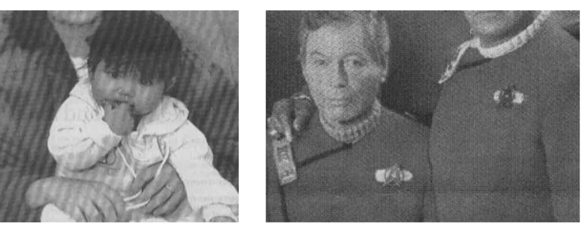
1.6 Examples of Ethic/race dierences. . . 8
1.7 Examples of pose variation. The top row frontal in plain rotation. The two to the left on the bottom row proles. On the right an example of face facing up. . . 9
1.8 Examples of occlusion . . . 10
1.9 Sketch diagram illustrates the main system stages . . . 16
2.1 Face normalization example. Left : raw face, right: face after normalization. . . 23
2.2 Edge image example. Left: edge image. Right: locations of the edges on the normalized face. 23 2.3 1-itemset support map (edge pixels scores) . . . 24
2.4 A scatter plot for instance scores . . . 25
2.5 Probability density estimate plot . . . 25
2.6 Sorted instances by edge score . . . 25
2.8 Fast Complex motion signals . . . 31
2.9 Fast and complex motions . . . 32
2.10 Video frame image and the cropping square . . . 34
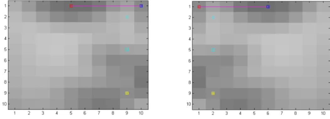
2.11 Intensity lter images that shows the estimated face features. Left is the original. right is the mirrored image . . . 34
2.12 Edge images. Left: original. Right: mirrored . . . 34
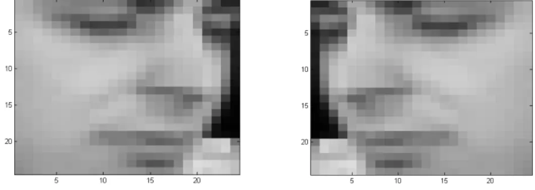
2.13 24×24 gray scale images. Left is the original. Right is mirrored. . . 35
2.14 Original gray scale image. . . 35
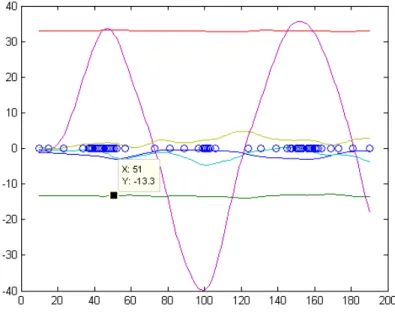
2.15 Pose signals plot. The circles on the line y = 0 are the interpolation points. The little black square is the data tool in Matlab. The box next to the data tool shows the reading value of the signal y and the frame numberx. . . 36
3.1 Frontal face maximal frequent itemset. Most of the MFIs collected with a reasonably fast computation interval form a frontal face edge map. . . 40
3.2 MFI mining results. All images except lower right are frequent patterns which pass the interestingness measure constraint. The lower right will be ltered out by the interestingness constraint. . . 41
3.3 1-itemsets support map for BU dataset . . . 43
3.4 Examples of quantile levels (I am showing only two levels). Right gure is for edges that have min_sup >66%. Left image is for edges with 66%≤min_sup >33% . . 43
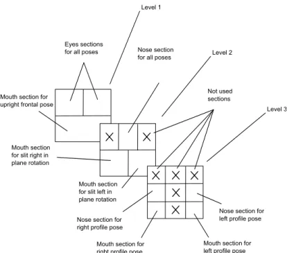
3.5 Face MFI mining levels . . . 45
3.6 Examples of face pose component sections. The left image is for level 1 right eye section. The image on the right is for left prole mouth section. . . 45
4.1 Finale detector design . . . 54
4.2 Image pre-processing steps that applied to the whole image and before any detection steps starts . . . 56
4.3 This gure shows an interfered signal wave has a constant frequency/length with the image signal. . . 58 4.4 This image shows the signal appeared on gure 4.3 after reducing the interfered signal
waves. . . 59 4.5 Extreme lighting condition problem . . . 61 4.6 This gure shows an original face image 4.6(a) and its intensity image 4.6(b). The
intensity image was depicted with the extracted facial features. The green circles are the local minima points as computed in section 4.4.2; as you can see in this image there are 7 points. The lter extracted the eyes and the nose as exactly the local minima locations since there is only one for each eye and the nose. While the mouth there are four points plus the nose location. The yellow dots show the mouth candidates and the points with the red stars are the main extracted features (eyes and mouth). the red square is the estimated mouth location after using the center of the eyes to further correct the estimation of the mouth location. The extracted samples are the (1) pixels between the eyes highlighted by the magenta line segment, (2) Mouth pixels highlighted by the yellow line segment, (3) left eye to left corner of the mouth pixels highlighted by the blue line segment, and (4) the right eye to right corner of the mouth highlighted by the cyan line segment. . . 63 4.7 Example of mouth to eye sample plot in a good lighting conditions. This plot is for
s(ml,l) sample but the right side is almost identical. Note that this plot is from real
data and it is for left eye to left corner of the mouth, so the point (1,0.2259) on
the plot represent the left eye with the lowest intensity value of0.2259and the point (10,0.3677)represent the left corner of the mouth with the intensity value 0.3677. . . 64
4.8 Example of mouth to eye sample plot in extreme lighting conditions. This plot is for the right side of the facesamples(mr,r)which is the dark side of the face. This
extreme case created by having the light coming from the left side, which in turn will illuminate the left side of the face but the right side will be dark. . . 65
4.9 Fitting curve for eye to mouth sample. Note that this curve was generated from formula 4.1 on step 7 in algorithm 9 and it is very similar to the ideal case on gure
4.7. . . 66
4.10 Good left to right eye sample S(l,r) . . . 67
4.11 Bad left to right eye sample S(l,r) . . . 67
4.12 Fitting curve for eye to eye sample. Note that this curve was generated from formula 4.2 on step 6 in algorithm 10 . . . 67
4.13 The applied sub-tting curveV(nl,r)to the right side of the sample vectorS(l,r)which is the sub-vectorS(nl,r). . . 69
4.14 Good mouth level sample . . . 70
4.15 Bad mouth level sample . . . 71
4.16 Fitting curve for mouth level sample S(ml,mr) in the case that left side was brighter than right side. Note that this curve was generated from formula 4.3 on step 3 in algorithm 11 . . . 72
4.17 Fitting curve for mouth level sample S(ml,mr) in the case that right side was brighter than left side . . . 73
4.18 Lighting correction examples: The upper row shows the original images. The bottom row shows the images after correction. The three images from left on both rows are for one location, and they are intensity,12×12, and24×24images. The three images from right on both rows are for another location, and they are24×24 ,12×12, and intensity images. . . 75
4.19 This gure shows how the in-plane rotation estimation algorithm uses the facial features locations to suggest a new rotated crop of the face that eliminate in-plane rotation. . . 79
4.20 . . . 80
4.21 Pyramid and detector stages illustration . . . 82
4.23 Sliding the scanning widow steps is based on the virtual 24×24 image not 26×28
image. Note the yellow strips are the margin areas where no detection is performed. 83 4.24 The nine resigns of the sub-window grid that the integral lter uses to compute the
the 36 Haar like features. . . 86
4.25 This image illustrates the concept behind the integral image. If we would like to compute the sum of pixels in rectangle 1 we compute S1=a+d−b−c . . . 87
4.26 Eye intensity search. This gure show the two cases. The case when both eyes location wasn't found using the local image, and the case when only one of them was found. The example here for the case 1 where only one eye was found is for when left eye was found and the right eye was not. Note that since the left eye is in the middle of the left eye search area then the algorithm will predict that the right eye will be some where in the middle of the right eye search area. . . 94
4.27 Examples for the facial features samples that the nal intensity classiers use to form its training features. . . 106
4.28 This gure illustrates the positions and areas that the rst local minima/maxima classier gets the samples for its features. The red crosses shows the locations of the eyes. . . 109
4.29 This gure illustrates the positions and areas that the second local minima/maxima classier gets the samples for its features . . . 110
4.30 This gure illustrates the positions and areas that the third local minima/maxima classier gets the samples for its features . . . 110
4.31 The right eye sample area for left prole. . . 112
4.32 The nose sample area for left prole. . . 112
4.33 The mouth and the cheek sample area for left prole. . . 113
4.34 The fth classier sampling area is vertical vector passes through the center of the visible eye. . . 116
4.35 The sixth classier sampling areas are two vertical vectors bellow the center of the visible eye. . . 117 4.36 The seventh classier sampling areas are three horizontal vectors one passes through
the center of the visible eye and the other two are blow it. . . 118 4.37 Left column images shows the extraction edges from full 24×24 upfront face image.
Right column shows the extraction of edges for full 24×24 prole face image. On the second row images for the cropped face after applying lighting correction and in-plain rotation variation elimination. Note how the prole elimination process produces edges for left prole face what ever the prole pose of the original face in the sub-window . . . 121 4.38 The nal MFI classier mining levels/sections design . . . 122 4.39 This gure shows a frequencies map for the edges of the unied prole sub-window. . 122 4.40 Fist Level sections. Left image is for the eye section. Right image is for the mouth
section. . . 123 4.41 Second Level nose section . . . 124 4.42 Third level, negative MFIs section. . . 125 4.43 An example of multi-detections. Note that the true face was multi-detected heavily
while other non-face sub-window was multi-detected less. . . 126 4.44 Multi-detections problem solving results. In this example I used the rst option which
is choosing an actual detected location that is closed to the computed mean location. The original detections are in yellow and the selected detections are in magenta color. 127
5.1 Example of processing and removing interfered detections. The locations that re-mained after applying the algorithm are shown in red. The dashed location is the original location reported by the multi-detections resolver algorithm. The solid red ones are the nal face location adjustment that will be reported by the detector. Not that the algorithm selected the location of the true face that was among the three interfered locations due to extensive detection score compared to the other two locations. . . 130 6.1 Number of discreet ROC curves of dierent algorithms in comparison to two types
of scoring methods for my algorithm. . . 146 6.2 Continuous ROC curves for the algorithms showed on gure 6.1 . . . 148 6.3 ROC curve of the nal design on MIT+CMU testset . . . 148 6.4 ROC curve for the integral lter and the intensity lter on 129 images with 511 faces
of the MIT+CMU testset using 0.9 downscaling. Figure 6.4(a) is for the integral
lter with step size 2. Figure 6.4(b) is for the integral lter plus the intensity lter
with step size1. . . 150
6.5 Option ROC curves. There are four curves one for each of the experiments mentioned in sub-section 6.5.2.3. . . 152 6.6 Perfect detection results with no false positives and accurate facial features extraction.153 6.7 100% detection rate with no false positives, but some facial features extraction was
not 100% accurate. The right image on the bottom row shows the original annotations of the features locations in blue, plus my detector extracted features in green and yellow just for compassion. As green means good, yellow means OK, orange means bad, and red means failed to extract the feature. . . 154
6.8 This two images showed me that my eorts to improve my design was successful eorts. The early versions were not able to detect the face without hundreds of false positives. The two images suer from extreme noise. The image on the left suers also from interfered long and low frequency signal. But the interference signals removal technique made this hard case an easy detectable face case. . . 155 6.9 Also shows 100% detection rate with no false positives, but some facial features
estimated locations was far from the actual feature. . . 156 6.10 Good detections for multiple faces in single images with no false positives. Even
though my training set didn't include any hand drawing faces but surprisingly the detector detected a number for hand drawing faces as shown in the right image. . . . 156 6.11 Good detection rate with acceptable false detections. . . 157 6.12 Low true detections with high false positives. . . 157 6.13 Images that form a huge challenge to the detection process as explained in section
1.1 paragraph complex textures. These two images have no faces but the detector found a huge number of false faces. . . 158 6.14 An example for the evaluation challenge where the detector successfully detected
all faces with no false detections but my evaluation measures rejected a true face detection and counted it as false positive. . . 159
1 Example of early versions of automatic cropping algorithm . . . 31
2 Semi-Automatic interpolation cropping algorithm . . . 32
3 Interestingness measure algorithm . . . 41
4 Constructing MFI search list algorithm . . . 48
5 MFI extraction algorithm . . . 50
6 Iterative Gaussian ltering algorithm . . . 57
7 Interference reduction algorithm . . . 60
8 Lighting correction algorithm based on average intensity . . . 61
9 Mouth to eye sample lighting correction algorithm . . . 65
10 Right side of between eyes sample correction algorithm . . . 68
11 Mouth level sample lighting correction algorithm . . . 71
12 Face sides specic histogram equalization as a lighting correction algorithm. . . 77
13 This algorithm estimates in-plane rotation and give new coordinates for cropping the face in a rotations the makes the new sub-window in-plane rotation free. . . 79
14 This steps executed only one time to estimate the right search size for the second level that will guarantee the nal size is the exact base size to prevent double scanning to near base size. . . 84
15 Integral lter construction algorithm . . . 89
16 Integral Filter: The Integral image based ltering algorithm . . . 90
18 Dimensions reduction algorithm . . . 129 19 Training section algorithm fro negative example selection . . . 139 20 Sensitivity enhancement algorithm . . . 141
INTRODUCTION
Face detection is a sub-problem of a more general and important fundamental problem in computer vision eld, which is object recognition. Face detection problem is dened by the problem of answering the question of whether or not an arbitrary image contains any number of arbitrary sub-windows that form an image belongs to the class of face images. And if there is any report how many, where are they located , and what size are they? Not to be confused with face localization in which the number of faces to be detected is provided.
The set of image faces is tremendously huge and the variation of the face appearance in an image makes it hard to construct a classication model that can discriminate all the variations of faces from other images that doesn't belong to human face class. It is hard because once the training set has a huge variation in the features that identify the class, then the decision boundary becomes unstable which reduces its accuracy.
Face detection is an essential part of any facial analysis algorithms like head pose estimation, face recognition, face verication and authentication and many other human-computer interaction (HCI) applications. The benets of introducing this skill to computational environments are count-less. This subject has been intensively studied. There have been hundreds of publications attempt to solve this problem in its upfront face detection. Example of remarkable leading solutions are like the work of Rowley [15] and the work of Viola-Jones [19].
A recent survey paper (published by Cha Zhang and Zhengyou Zhang [20]) covered the work that has be done for the past two decades. It provided a great explanation of Viola-Jones integral
images based object/face detection algorithm. They reviewed a number of dierent features, a number of learning schemes, and a number of detector structures.
The fundamental components of a face detector are image pre-processing, pyramid scaling and scanning locations generating, classication/ltering models, and multiple detection resolving. The construction phase of building a face detector consists of training data collection and preparation, training sample design and preparing, model selection, training, eciency/performance enhance-ment, tuning/adjustenhance-ment, and testing.
The rst paragraph of this introduction presents face detection as a sub-problem of object detection. And the second paragraph mentioned the variety of face appearance. The variety in-cludes; noise, brightness, contrast, lighting conditions, ethnicity, race, age, sex, occlusion, and head pose. Based on the head pose variations, there have been solutions target a small sub-set of pose variant. This solutions attempt to reduce the variety of face appearance by solving a small section of a larger problem.
The most common sub-set of the face detection problem is upright frontal face detection. This domain is the most studied aspect of the problem, and most advances accomplished in face detection are in this domain. The in-plane rotation face detection is a rotated frontal face detection problem, it is also well studied and accomplishments are achieved. The third domain is the upright prole face detection, there have been a quite good number of approaches with low detection rates. The most dicult type of face detection problem is; the variant pose face detection in uncon-trolled environments. This class of the problem or the complete set of face detection problems is poorly studied and very few solutions presented. The accuracy and precision of these solutions are not clear. And a standard testing and evaluation for compression is not available.
The goal of my thesis work is to design and construct face detection algorithm that is pose invariant under uncontrolled environments aimed for head pose estimator to be used in human-computer interaction (HCI) application. My current suggested system doesn't address the full head pose variation. It addresses only the important to normal (HCI) application needs. These needs are; ability to detect in almost full prole for both sides (i.e about±80◦yaw) combined with partial
in-plain rotation detection (i.e about ±45◦ roll) and with partial pitch angle (i.e about ±45◦. A
pitch angle is the angle that measures whether the face is turned up or down. Refer to [14] for graphical explanation of pitch, roll and yaw).
Even though the solution I needed to build is not the full case of the problem. It is still as hard as the full pose variant detecting case. My proposal is to build a single classier cascade based detector that incorporate a data mining approach and performance/pose customized classiers suitable for multi-pose detection. This thesis is about designing a face detector algorithm that is robust universal semi-pose invariant under uncontrolled environments.
The design of the proposed detector have been achieve after a massive development and design changes. I started with a single classier detector and ended with an ultimate multi-layer cascade of classiers design. The design was guided by the performance and test results.
Test was performed and measured using a recent published benchmark (FDDB: A Benchmark for Face Detection in Unconstrained Settings [12]). Results of similar solutions on variant pose testset to compare are unlivable. The results using FDDB [12] system and compared to the upright frontal solutions show a very low detection rates. In the next section I will discuss challenges and diculties in building a general face detection system. Then I will present my approach to building and evaluating the proposed solution. I will end this chapter by an over view of the organization of the rest of the document.
1.1 Challenges and diculties
A number of challenges and diculties reduce the eciency and accuracy of any face detection algorithm. These include noise, brightness and contrast, lighting conditions, complex textures, pose variation, scaling and transformation, and occlusion. Rowley [15] presented a useful overview of the problem in his thesis. Also there are other challenges related to building the detector such as nding or creating a good training data set, labeling the data, training data selection and pyramid scaling. These data quality challenges aect accuracy, detection vs. false positive rates and speed.
size and any location of a possible face in the image (see gure 4.21). The detector must classify each window as a face or non-face. This typically requires a machine learning based model trained using examples of positives and negatives. When dealing with face detection in uncontrolled environments we have to consider in our positive examples the variation and the challenges mentioned above. This unfortunately increases the complexity of the decision boundary and leads to reduction in eciency and accuracy. As part of the challenge the detector has to deal with each diculty and variation in a suitable way. Part of handling these variations is by using basic image processing techniques like smoothing and histogram equalization. Another part of the solution is to choose the right features at each stage. An other type of challenge comes from the type of methods and models that we use to solve statistical problems. Most of machine learning algorithms that I am aware of are; when applied to an average problem usually do not do better than 0.1% error or 99.9% accuracy.
Face detection is hard inseparable problem that the average rate is higher than 2% error or 98%
accuracy. That is extremely high and in practice it gives rather poor results due to the unbalanced distribution false/true examples and the high volume of non-faces that exist in real world images.
In the next paragraphs I will review the challenges for face detection described by Rowley [15] with reference to my own practical experience are as follows:
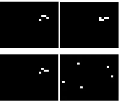
Noise Is very dicult problem. From practical experience images that are too noisy are hard. When scanned with the detector the results are high number of false positives and low detection rates. Noise turns smooth background texture into complex textures that easily pass all the detector stages. On the other hand noise alters the features of true faces creating more complex textures causing the face to be rejected. Examples of noisy images are shown in Figure 1.1.
Brightness and contrast Variation in brightness and contrast adds some complexity to the clas-sier. For example we think of the face as an object that will have dark regions like the eyes and mouth and bright spots like nose and cheeks. Images with poor contrast will be
Figure 1.1: Examples of noisy pictures that suer bad detection rates and high false positives.
very hard for a computational model to distinguish as these features will be poorly dened. A similar degradation of standard face appearance occurs with low or extreme brightness. Imagine an image where the brightness of the eye is higher than the brightness of the nose in other images. This kind of variation makes the decision border unstable. Examples of brightness and contrast variations are shown in Figure 1.2.
Lighting conditions This is an interesting problem. Here we are faced with the fact that images of faces are generally not captured in controlled environments like labs or photography studios. The ideal face lighting has the light sources directly in front to minimize self-shading and ensure that the face is evenly lit. In the real world this is rare. The worst cases are when half of the face is extremely lit and the other side is extremely dark. Designing a classier to handle this case is almost impossible, because adding examples that suer from bad lighting conditions will aect the decision boundary and cause more false positives and very low detection rates. Examples of extreme lighting conditions are shown in Figure 1.3.
Complex textures This was the most challenging problem for all versions of the detector. Con-sider an image of trees, book shelves, or a newspaper, the complex textures of these scenes are similar to noise. This problem is magnied when noise is present. Part of the problem
Figure 1.2: Examples of brightness and contrast variations
is the complex intensity variation forms false face like featurese.g nose eyes and mouth. Unlike human eyes and brains which are ecient in recognizing context and textures and ignoring them, mathematical models seem to be unable to distinguish between true and false positives within rich textures. Humans are not limited to a single static view, and can use hybrid techniques and models, for example we may use the context of the body also. For computational models it looks like using a huge number of features as in Viola Jones [19] was really rewarding.
Beyond complex textures, problems can arise depending on how faces were cropped in the training set. In this work faces were cropped very close to the mouth and eyes to minimize the eect of hair style, beards, and backgrounds. Unfortunately there are many non-faces that when you crop them in the same way, would form very face like appearance that is very hard to reject even for the human eye. Examples of complex background textures that produce a high volume of false positives are shown in Figure 1.4. Examples of hard negatives are shown in Figure 1.5.
Ethnicity and race This is also a source of complexity. This problem arises when the size, location and shape of the face featureslike eyes, nose, mouth, cheeks, etcare dierent from person to person, from age to age, and from race to race. Constructing a detector that can recognize all the variations is a challenge. Using examples of dierent races essentially dilutes the model and introduces more false positives. Examples of ethnic/race dierences are shown in Figure 1.6.
Head pose By examining frontal upright faces one can nd common characteristics where features like eyes and mouth consistently appear in similar locations. This makes building a machine learning model for this case quite reliable as demonstrated by most successful front face
de-Figure 1.4: Examples of complex background textures that produce high volume of false positives
Figure 1.5: Examples of hard negatives. Notice that some of the examples look like faces with eyes, mouth and nose.
Figure 1.7: Examples of pose variation. The top row frontal in plain rotation. The two to the left on the bottom row proles. On the right an example of face facing up.
tectors. However, multiple variations of poses like in plane rotation, out of plane rotation, scaling and transformation will make the locations of these canonical features change dra-matically. Pose variation can also make the lighting of the face surfaces vary in unexpected ways, making building a model very dicult. Examples of pose variation are being shown in Figure 1.7.
Occlusion In face detection problems we usually train a detector using perfect examples with no occlusions. This may result in bad detection for partially occluded faces. If few occluded faces are being used, it may produce models that have bad detection rates and high false positives. Using many examples of occluded faces will result in a poor discriminator. Oc-clusion changes the appearance of facial features and that adds extreme variations to the training examples and complicates the decision boundary. In my training examples there are no occluded faces. This makes my solution work on non-occluded faces better. Occlusion would include sun-glasses, hats, beards, partially covered faces by hand and other objects that could be present between the camera and the face. Examples of occlusion are shown in Figure 1.8.
typi-Figure 1.8: Examples of occlusion
cal machine learning problem where tests are made on50%positives and50%negatives. For
example for the traditional frontal face testset MIT+CMU dataset there are 118,766,602
sub-windows when scanned using a downscale of .9 (or ≈ 1.11 in bottom up scaling) and
step size 1 (scaling and the pyramid will be illustrated in Section 4.3). I have to mention
here that I am using only 111 images out of the 130images. That is because some of the
images have hand drawn faces and my detector was designed to detect real faces. Some other images were not recorded in the ground truth also my detector doesn't scan them. In these 111images there are only 489faces and all other windows at all scales are non-faces.
On average, an image has about 1,069,969 sub-windows with an average of 4 faces and 1,069,965sub-windows are false positives.
From the machine learning perspective, if we can build a model that has99%accuracy and 1%error, it will be considered an excellent success. But let us see what that means in face
detection: 1% error for 1,069,965 is 10,699.65≈ 10,700 false positives. Add to that the
fact that usually not all the faces are detected correctly anyway. An algorithm with only
1% error rate will be considered unreliable and inappropriate for face detection because
of the false positives rate. We need an algorithm that has close to 0.0003% error rate and
accuracy of 99.9997% to have an average of3 false positives/image.
and 99.9% success on an average problem, and more than 15% error on hard inseparable
datasets similar to multi-pose face detectionat least for all the features that I experimented which I couldn't nd good separable features. If we can construct a face detector with an error rate of .001% there will be about 1,069 false positives per image with 1,069,969
sub-windowsif such features and algorithm can be found.
Training dataset Finding or creating a good data set is not an easy job. As I mentioned in above paragraphs building a detector for a limited class of the problem (e.g. Upright frontal with normal lighting conditions face detector) is easier than a detector that can work in any conditionsI am saying easier! But I don't mean easy. The diculty of building such detector doubles for each variation that the builder would like the detector to solve. Finding a training dataset for the upright frontal face detection is not as challenging as nding or creating a dataset that includes any face variation (e.g. all possible lighting conditions, all possible head poses, all possible ages and ethnic variations, etc.), which I think is impossible. The all poses or multi-view detection problem is harder than the upright frontal problem and has lower detection rates. Attempting to solve the multi-view detection by only one detector is a very hard problem and nding or creating a training dataset for this problem is much harder than upright frontal. There are many approaches in the literature to solve this problem in this fashion as in [13]. Some solutions suggested creating a detector that is made from combining a number of detectors where each was trained to solve a small domain of the problem as in [1]. The problem with these solutions is that each sub window has to be checked by each individual sub-detector which is very expensive computationally. In my approach I tried to solve the problem using one detector which results in low detection rates even for frontal face testsets.
Labeling Labeling the training dataset remains the hardest and most expensive task, but yet it is a very important issue. I searched the web for a free good labeled training dataset and couldn't nd one. Each face detection published work the writers created their own labeled
training set by manually labeling each face individually. Some have created or used a manual labeling tool but yet it is still done manually. To clarify the problem, in most published work they used about 10,000faces as positive examples to train their classiers. Labeling
this huge number of faces is a hard task and it is very dicult to check the accuracy of the labeling. In my work I tried to use an automatic/semi-automatic solutions that made that task about 10 times faster than using a manual labeling tool. But my solution is not fully
automatic and it is still time consuming to manually check the accuracy of every labeled face.
Training data selection In this paragraph I would like to present another class of wonder and it is about the negative examples selection. The problem is the number of all possible examples that can appear on a 24×24 sub window of 256 gray scale image is 256576 ≈
1.4×101387. I assume that almost all of them are negative examples and the fraction of positive examples to the negative is very small. The question is what sort of negative examples should be selected and will be eective in training? Especially since the number of my labeled positives is limitedit is preferred to train machine learning algorithms with an equal size of negatives and positives. Also using a large training sets is very expensive in both training and detection times.
Another question is since I have a hierarchy of classiers, how the selection of the negatives for each classier should be formed? Should I use the same set for each classier, or should I just randomly select sub-windows from a random images and form a dierent training set for each classier. The approach that I followed is similar to the Viola Jones [19] approach, which is the selection is based on the false negatives that pass previous layers. The algorithm is explained in section 6.1 in detail.
Two problems with this approach, rst is when my training process reaches the last layer in the case there are more than six layersthe training process will reach a point where the partial detector doesn't pass any false positive to the next layer even with images
containing complex textures. It seems like we have reached a perfect face detector! Nope, when testing this partial detector on testsets these tests showed that nothing can pass even faces that are ideal in all variations.
The other issue is when using such detector and by easing the thresholds of all the classiers to allow better detection rates, how good is the detection rate vs false positives rate. It depends on the quality of the features of all layers, but in general my experiments showed that we get quite low detection when we reach a low false positives. Another phenomena, is when I lower the threshold the false positives that used to be rejected by previous layer passes to the next classier that has never been trained on similar examples and so most of this hard negative examples will pass all the way through the next layers. In other words the decision boundary is aected by missed negative examples in the training process. The way that we tried to solve this problem is by lowering the threshold during the data selection process. I mean by changing the threshold and changing all classiers models decision boundaries thresholds to let faces/non-faces pass (The models include the integral lter, intensity lter, and all machine learning model like PAM models, SVM models, ... etc. At the time of writing I have conducted no experiments to explore the results of such approach.
The Threshold lowering process is done in two ways rst automatically on the training set until all positives can pass. This was a good fast way to predict how well the classier being trained will do on future sets and an early decision can be taken immediatelywithout waisting more time on testingwhether to keep it or design better features. I start this automatic process by lowering the threshold iteratively by small decreases in the threshold and compute the specicity and sensitivity on the whole training setmore like ttinguntil I reach a desired sensitivity. In my last version I used 100% sensitivity on training data.
Then I check the specicity, if it is above a desired rate I keep the classier otherwise I would replace the classier using dierent features. This approach enhanced results in testing time by allowing better detection rates.
This approach worked for a number of classiers where I was able to collect false positives, but when the cascade reached the last few classiers to train the partial detector allows no more false positives. In other words the problem of running out of false positives examples still exists, so a manual threshold adjustment was needed. This manual adjustment focused on the number of false positives that are allowed to pass to the next level so at the end of the cascade I can guarantee that I can nd false positives for the last classier training set. As an automatic benet of this method in detection time when adjusting thresholds to improve detection rates the false positives that pass the current layer are highly likely to be rejected by the next layer, since chances are the next layer has learned about its sample class example during training time which in turn should improve detection rates and lower false positive rates.
Scaling and scanning the pyramid This is a design and implementation issue. Recall that the discussion on unbalanced distribution on page 9, the gures in that section reect 0.9
downscaling of the scanning window (which is approximately1.1111 up-scaling in [15, 19]
algorithms in which they start with base scanning window then they upscale for the next pyramid scale). The0.9downscaling is the maximum that for any image before the pyramid
scales start to overlap which is a waste of time. I mean by overlap is to repeat the same size of the scanning sub-window because of the discrete nature of pixelization. The overlap occurs when the downscaling reach sizes close to base size (which is the smallest size). Choosing0.9downscaling guarantees that the scanning will cover every meaningful possible
scale in the pyramid which in turn increases detection rates. The downside of this is that it produces a huge number of sub-windows to scan which slows the performance and requires a large amount of memory. On the other hand using scale of0.5(2in [15, 19]) results in fast
detection speed with very low detection rates. The question that a face detection designer has to answer is: what scale is perfect for their application?
the scanning sub-window should be shifted to scan the next location. This shifting process is aected by sub-window scale size. Let the base step size be δb and the base scanning sub-window side be zb. The step size factor will be δbzb. At any pyramid scale I adjust the step size to a relative size of the scanning window. Let the scanning sub-window size bezw then the the step size for the sub-window sidezw will be δw = δbzbzw.
As my base scanning size is 24×24 so the base side size is zb = 24. In order to cover all possible locations at every pyramid scale for 0.9 downscaling, the base step size δb has to be set to 1. When choosing a downscaling factor of 0.9 and base step size that is 1 the
number of total sub-windows per image will be extremely big which aects the speed of detection process. Choosing a step size of 2 dramatically increases the speed of detection
and decreases the detection rates. The same question here is what base step size I should choose?
1.2 Approach
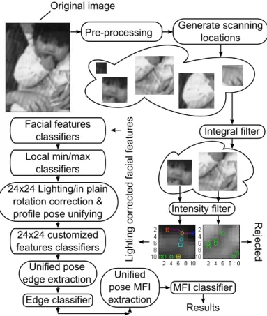
The work described in this thesis represents an extensive iterative renement of approaches I worked on over a two year period. Our initial goal was to estimate head pose for user interaction which requires a face detector which can nd faces in the image at a range of in-plane and out-of-plane rotations. A face detection system has two parts or phases: model construction from labeled face and non-face examples, and the nal deployed detector which applies any required image processing and pyramid sampling to evaluate the model and report detected faces. Figure 1.9 presents a sketch picture of the proposed system. The following paragraphs reviews the two main stages in this system.
1.2.1 Model Construction
Model construction includes data collection and labeling then model training and testing. After evaluating a number of datasets I choose to work with the Boston University (BU) dataset [5, 4] and constructed a semi-automatic technique to label face windows from video frames using
associated pose data, then manually cropped interpolation points. In the training phase I started with a pre-lter that uses the integral image [19]. The integral image lter was built by collecting the positive face feature samples from positive integral images then by applying some measurements that lead to clustering like technique. Next is learning the intensity lter. This lter also measures and learns from positive examples only. It performs a novel facial feature extraction for eyes, mouth and nose. Next, using the extracted features a classier cascade is trained.
Negative examples are being collected so that at each level, classier fi uses the previous already trained parts of the detectorf1, f2,· · · , fi−1 to scan a collection of images. For rst versions of the detector I used the CBCL Dataset [6] to extract negative examples. But then due to unsatised requirements I switched to the Caltech dataset [3] which has faces but face windows have been excludedso that at each level fi will be only trained on the negatives that the previous level fi−1 failed to reject. This technique will be used for all next levels of the cascade. The algorithm is explained in section 6.1 in detail.
The rst group of classiers of the cascade uses features computed from intensity samples for the facial features reported by the intensity lter. Next was to train texture based classier features. The classiers measure the changes in intensity that produce local minimas/maximas to describe the texture of the image. Next and in the last version only I add a number of classiers that use a variety of high volume features. Next is trained edges classier. Finally the MFI (Maximal Frequent Itemset) Classier is constructed starting with collecting edges of positive examples then mining them, clustering, them, forming a search tree, preparing the negative and positive samples then training.
1.2.2 Detection phase
This part is the live part: the product that will be used on-line. It is also the main part in evaluation. Detection starts with image pre-processing: normalization and noise reduction, compu-tation of the integral image and preparation of scanning locations. The integral pre-lter is applied. This will eliminate most of the false positivesdepending on the threshold and image complexity.
The intensity lter will eliminate many of the remaining false positives that passed the pre-lter. Facial features are extracted and their brightness will be corrected by the intensity lter. Next are the intensity classiers that will reduce more false positives. Followed by the texture cascade which apply no lighting correction, but the rest of the detector levels use the information from the intensity lter to correct the lighting and the pose of the face. Next is the customized features classiers cascade will be applied, followed by the edge classier and the extraction of MFI itemsets and then the application of the MFI classier. Finally resolving the multi-detections (Some of the faces are detected multiple times and a single response must be selected).
1.2.3 Evaluation
The evaluation of a face detector is not as obvious as it seems to be. The early published papers (e.g. [15]) collected and prepared their own evaluation testsets. Later papers used these collected early testsets to compare their work to these early algorithms. An example of such testset is the famous MIT+CMU dataset. Which was created by Schneiderman and Kanade [16] where they combined the work of Rowley [15] and the work of Sung [17] and added more prole examples to produce the testset known by MIT+CMU testset which was used in a CMU face detection project. There are two problems with these evaluation testsets and the evaluation algorithms that they created. One is the problem of the testsets is that they were created by the same algorithm designer and the testsets are very similar to their own training sets in terms of quality, noise lighting and pose variations. Which will reect high detection/false positive rates that do not reect the real performance due to the fact that they are all form a subset from the real world face images (i.e all testsets and training sets form the same subset).
The other problem is the problem of using non-standardized evaluation algorithms which will lead to: rst, biased results and second, no standardization for others to compare their work; because each algorithm writer dened a dierent standard to consider a good face detection. For example when I was designing my evaluation algorithm I asked myself the question; if the detected face was not in the middle of the detection window, in other words if half of the window contains
half of the face and the other half shows the background, should I evaluate this as a true positive or a false positive? For details about my evaluation algorithm refer to section 6.3
As an example that an old literature didn't show real results is to look at the work of V. Jain and E. Learned-Miller [12] which showed that [19] has 39.41% detection rate with 0.6 false
positives/image when tested with FDDB [12] testset. Whereas [19] in their paper on MIT+CMU testset reported92.1%detection rate with.6false positive/image. Jain and Learned-Miller [12] have
developed a comprehensive testset called FDDB that includes more aspects of faces and a variety of background textures than all other testsets. They also created a common and standard system for evaluation.
Unfortunately the FDDB [12] testset is more than 21 times larger than MIT+CMU which
due to time constraints I was not able to extend my thesis in order to include tests on multiple operating options using this testset. I became aware of this work just about six months ago while I was in the middle of constructing my last versionconstructing and training new face detector takes about two to tree months.
The way that the FDDB evaluation algorithm was designed was dierent from my evaluation specication. A complete reconstruction of the detector was needed to change the scoring system. This eorts introduce new bugs that took extra months to rebuild the detector and about a month for testing. I conducted only one test that is the over all performance under specic set of options. Back to the challenges regarding two dierent sets of training and testing. I had constructed my training data from ve subjects in 14 videos from the BU [4] dataset. There are 2534 original
framesor faces. In order to double this number, images were mirrored and added to the collection to achieve the sum of5068 face examples that vary in head pose and lighting conditions.
The MIT+CMU and the FDDB oered a huge challenge for my system. Which means my training dataset, the MIT+CMU testset and the FDDB testset are from completely disjoint sub-sets as their super-set is the real world of all possible images of faces and non-faces.
The huge dierence between my training set and these testsets was meant to mimic the situation that could happen if images are being scanned completely from a dierent domain and
have never been introduced to the learning process. This provided a real test for my system and how it will preform when faced with absolutely never seen test examples. Experimental evaluation was done to explore the performance of the detector. Included in this thesis are graphs and a table that will illustrate the results of my work.
1.3 Thesis organization
The rest of this document is organized as follows; Chapter 2 will provide information about the collection and processing of the data that can be used for training an appearance based multi-pose face detector. Chapter 3 explains the use of the MAFIA algorithm in constructing a face detector. Chapter 4 will explain all preparation steps, pre-ltering and building all types of the used features and their cascade classiers along with multi-detection resolution. Chapter 5 will show all the design decisions toward eciency and accuracy. In addition to that the use of multi-threading and other solutions for computational speedups. Chapter 6 Will cover all the evaluation issues from training to evaluation algorithms and evaluation data. It also will present experimental results that measure the performance of the constructed detector. These experiments target some aspects of the detector performance. I will end this report with conclusions and future work in Chapter 7.
DATA COLLECTION AND PRE-PROCESSING
2.1 Introduction
In this chapter I will discuss the issues that accompany preparing a training dataset. A training dataset for a machine learning algorithm must include positives (faces) and negatives (non-faces) in equal amounts. At the beginning of this project I used LFWcrop Face Dataset [11] then due to unsatised requirements of the application I evaluated a number of other datasets including datasets to extract hard negatives.
Recall what I mentioned in section 1.1 regarding the training dataset. One must address all the issues in section 1.1 when preparing a training dataset. As I mentioned it is not an easy job to nd or create a decent training set. One may think that nding a ready dataset for training is easier than creating one. For a head pose problem, yes it is. Since a good training set must be provided with a robust ground truth measured using an advanced and expensive technology which is rarely available to only very small number of students/researchers.
For face detection one can create their own dataset using any commercial camera. Then manually labeling the location of the faces which is the problem since it is a hard job when it comes to labeling huge amount of images. I chose to nd a ready made available dataset on the Internet. There are many problems with such datasets; rst without a manual examination one cannot guarantee that they are good training sets for the purpose that the detector is being built for.
(HCI) application that requires the detection of a face in a variant poses. Even though that I didn't need full rotated faceslike upside downbut faces with a natural rotation like the one that a standing up person might rotate his/her face. Which about−45◦ to +45◦ in plane rotation and
with a pitch in a similar range. And almost a full prole which is from −80◦ to +80◦. But nding
such a data set is not easy. And as I said the manual examination for all images in the set to ensure that the dataset includes all the poses is necessary.
Another problem is that most of this data was created in a prefect lighting environment. My dataset has to include extreme lighting variations which is very hard to nd in a ready dataset. Also a variation of ethnic and skin color, etc. Let us say that such dataset was found and it is guaranteed that it covers all the requirements of the purpose. This data set usually will not be labeled or badly labeled, which means I need to label it myself. Labeling it manually is just not a fun task when I have over 5000 images. In this chapter I will present the processes for preparing
such a data set and the automatic labeling solutions and their pros and cons that I tried.
2.2 Face Datasets
At the beginning of this work I searched for a good data set. Since I was planning to con-struct a pose estimator, datasets were evaluated based on the existence of measurements for pose information, the quantity of variant poses, and ready cropped faces for detection training. Dataset choice was based on recommendations from Murphy-Chutorian's survey [14] which emphasized the accuracy of the pose measurements, but availability was an issue. Datasets with pose measured using the most advanced technologies are not available for academic research. Those technologies include Optical Motion Capture System (best accuracy), Inertial Sensors, Magnetic Sensors, and Camera Arrays. The Boston University (BU) Face Tracking dataset [4] is freely down-loadable, with pose captured by Magnetic Sensors. The data set is not perfect it suers noise in the measured signals and a delayed response as illustrated by Murphy-Chutorian et al. [14].
The other datasets that I used at rst were LFWcrop Face Dataset [11]. This dataset was ready cropped which I thought it will be suitable for mining MFIs and detection training. The
Figure 2.1: Face normalization example. Left : raw face, right: face after normalization.
dataset CBCL Face Data [6] provided a large amount of cropped frontal faces as positives and a dicult non-face instances. I discovered that the frontal faces are useless for my mining and detection training for two reasons (1) They are only for upright frontal pose; (2) the size of the images is too small for the mined edges to be meaningful. At that time the non faces examples I thought were perfect, but I later discovered that they are not enough. I needed more examples of cluttered backgrounds and with 24x24 resolution so I used the Caltech data set [3] to extract the non-face examples only. In the following sections I will talk about each dataset and its characteristics and steps that were required to make it ready for classier training.
2.2.1 LFWcrop Face Dataset [11]
This dataset is a cropped version of Labeled Faces in the Wild (LFW) dataset, created by The Computer Vision Laboratory, Computer Science Department at the University of Massachusetts. In LFWcrop (cropped Labeled Faces in the Wild) dataset there are 6862 instances of all positive
faces. It was prepared for face recognition problem. At the beginning, I thought this will be my positive set. But after I did random examination on the images for the purpose of conrming that it represents an acceptable dataset for face detection. I also did some data pre-processing by applying normalization (see Figure 2.1). Which results in a high contrast image to improve edge detection (see Figure 2.2).
Figure 2.3: 1-itemset support map (edge pixels scores)
Since this was the start of the project I wanted to explore whether there will be any frequent patterns. I computed the frequency of each edge pixel and created gure 2.3 for graphical represen-tation of the pixel frequency. Then I was interested in creating an image scoring based on edge pixel frequency map. Basically for each edge pixel in the positive example I look up the score for that pixel then I sum all the scores and that will be the score of the image. By computing image edge scores and analyzing max and min scores. As an experiment to check if I can create a fast pre-lter as a part of the detector, I discovered that the range between minimum score and maximum score is extremely wide and a lter could not be constructed on this basis. This property interested me and got my attention to check if the dataset may not form a good source for training.
Before taking any decision I used some simple data mining tools to further analyze the data. A scatter plot was generated for the edge scores (see gure 2.4) and a probability density estimate plot (gure 2.5). These two plots show that some instances have extreme scores in both directions. The normal distribution of the data was symmetric. To analyze even further a sorted quantile plot was created (see gure 2.6). The scatter plot shows that there is some sort of a pattern but also there are extreme outliers.
By examining these interesting plots I started to ask the question, If these are all frontal upright faces why do we have these instances that form some sort of outliers? My assumption was that they should all have similar edge scoringwhich is wrong after I became more familiar with the subject and that is because the extreme variations like pose and lighting conditions etc. will produce dierent scores. At that time and after another examination on the edge score map and
Figure 2.4: A scatter plot for instance scores -0.5 0 0.5 1 1.5 2 2.5 x 10⁵ 0 0.2 0.4 0.6 0.8 1 1.2 1.4 1.6x 10 -5 Instance score D e n s it y
Figure 2.5: Probability density estimate plot
0 1000 2000 3000 4000 5000 6000 7000 0 0.2 0.4 0.6 0.8 1 1.2 1.4 1.6 1.8 2x 10 5 Sorted instances S c o re
since it looks like there is a some sort of a frequent pattern I asked the questions Are most of these images frontal? and What do the images with lowest score look like?.
By identifying the images original indexes and displaying the low score images, I discovered that most of the lower score data is noise, i.e. they don't form a complete face or they are badly cropped images. At the top there are good frontal face images. Also based on the scoring map I predicted most of the the images are prole faces. I concluded switching to a dierent data set was necessary.
2.2.2 Boston University Dataset [4]
This data set consists of about 75 videos; each video has about 200 frames. This dataset was prepared for head pose estimation by the Image and Video Computing Group at Computer Science Department, Boston University. The dataset provides pose ground truth. Not all videos are labeled. The pose measurement technology is a Magnetic Sensor. I was only able to use 14 videos with a total of 2534 frames which is the total number of positive instances. To increase the number of positives a mirroring of each face image was calculated and that doubled the total number of positives to 5068 faces. Since this is a video database, examining it to conrm the satisfaction of the requirements was easy by just watching the videos. And no data analysis was required as in Section 2.2.1.
This dataset is not cropped for face detection training, since it is intended for head pose estimation. Instead of manual cropping, I implemented an automatic way to crop faces using the pose data. The pose data is quite noisy. In the next sections I will explain how to reduce this noise. I have to say that in the later versions this pose data wasn't used in the face location estimation problem instead I used interpolation to interpolate a number of manually cropped windows of face regions in each frame. Then estimate the other frames face positions. In section 2.4 I will explain this algorithm in detail.
2.3 Non-face datasets
In this section I will talk about the two datasets that I used to extract negative examples. I rst used CBCL Dataset [6] for my rst version of the detector. I thought that it will be easy for me to use a ready selected negative examples, since I have no experience about how to construct a good negative examples dataset. But later with more experiment with false positives issues I searched for a dataset that is more natural and close to real world negative images that can be found around positive or face images. I selected Caltech Dataset [3]. Then following sections will present this datasets.
2.3.1 CBCL Dataset [6]
This data set was created at MIT. As mentioned above this data set has a low resolution for edges, but it provided the project at early stages with 4500 negative instances that were very similar to real faces. Visual examination for a small fraction of those non-faces, will nd that many have face-like features. At that time I didn't mind that the size of the non-faces was 19x19 where my face examples were 24x24. For a machine learning training data all negative and positives have to be the same size. I needed to upscale the negative examples to 24 x 24.
When the rst detector was built and tested using the standard machine learning future error on unseen data, we observed future error estimates of 3% for 50 experiments. That is 97%
accuracy. Unfortunately this error estimate is not appropriate for face detection problem where the distribution of the data is not balanced as I mentioned in section 1.1 paragraph Unbalanced distribution. For the standard image pyramid used for face detection this is not a good resultif we have an average of 382,295 windows/image 3% means about 11,469 misclassied windows or
false positives/imagesince an image has in average less than 10faces.
By realizing this shocking fact and my awareness that no machine learning algorithm has accuracy reaching99.9999% accuracy on inseparable data, I understand why researchers like Viola
a cascade of classier to exploit a variety of dierent features. My experience also led me to realize that non-face examples must be extracted from pictures with backgrounds similar to real life and so the dataset Caltech [3] was introduced.
2.3.2 Caltech Dataset [3]
As mentioned above I was looking for background images that reect to real world examples. This dataset is a frontal face dataset, created and collected by Markus Weber at California Institute of Technology. The dataset contains 450 frontal upright face images was taken under dierent
lighting conditions and a variety of backgrounds. The backgrounds are ideal; they include trees, grass, book shelves, dark rooms, oces. etc. As I mentioned above this dataset contains faces that I have to avoid extracting them as a negatives. Using the ground truth information I excluded the face windows and only collected non-face windows. There are some unlabeled faces in the image backgrounds that needed to be manually examined and processed.
All images have the same size896×592, which produces about2,328,830sub-windows/image
if scanned with a scaling factor of0.9and step size 1. The total sub-window over all the dataset is 1,047,973,500 sub-windows. I also used each image in 8 dierent variationfour 90◦ rotations for
both original image and mirrored imagewhich total the negative sub-window that are available as examples to8,383,788,000sub-window.
2.4 Labeling
In this section I will present the techniques for auto-labeling and cropping for the positive data set. I start with explaining a simple technique I used to clean up the pose signal. Then I will talk about my attempts to use this data to estimate face location for auto-cropping. I will end with an interpolation technique for semi-auto-cropping and a cropping tool to create interpolation points.